
Clustering Method for Load Demand to Shorten the Time of Annual Simulation

 ,
, 

Abstract
:1. Introduction
Clustering Method
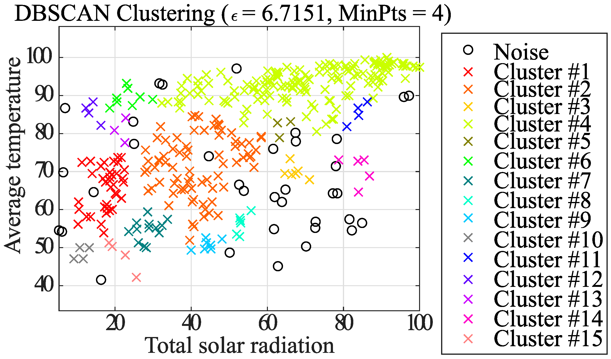
2. DBSCAN
2.1. DBSCAN Method
- (1)
- Label the elements of the data set based on the following three conditions
- A core point is a point such that there are at least the specified number (MinPts) of adjacent points within the specified radius .
- A border point is a point such that the number of adjacent points of radius is less than MinPts, but is located within radius of the core point. In Figure 1, the center point of the red dotted line is the boundary point.
- All other points that are neither core nor border points are considered noise points.
- (2)
- Clusters are formed for each core point. If the core points are within radius of each other, they are assumed to belong to the same cluster.
- (3)
- Assign each border point within radius of the core point to a cluster of that core point.
2.2. DBSCAN Adaptation Methods
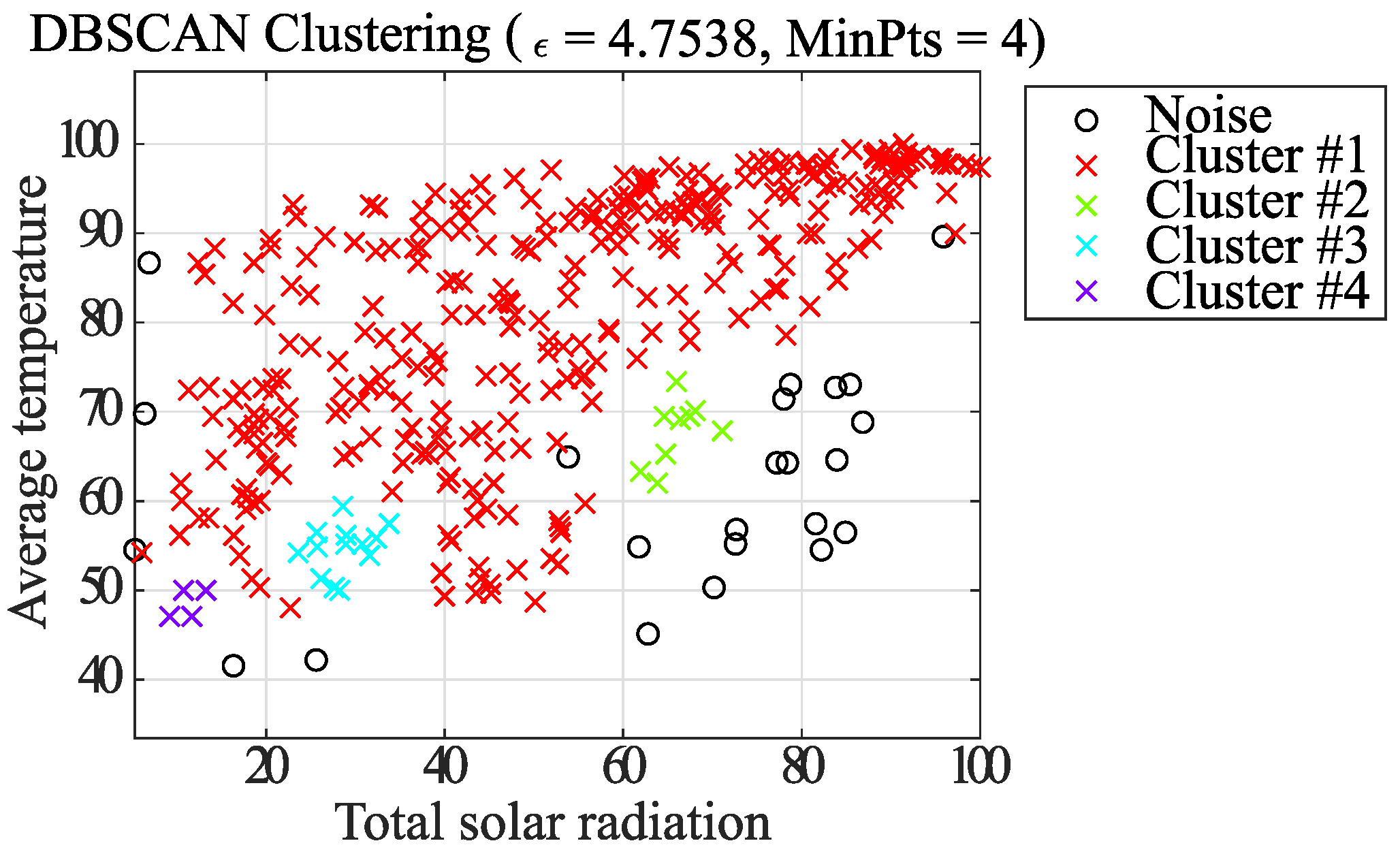
- Percentage notation conversion formula for each data valuewhere X: the set of data for 365 days, : the set of data for 365 days (after percentage transformation), : the i-th data value after percentage notation transformation, : the i-th data value in X, is plotted on the two combined coordinate planes.
2.3. DBSCAN Implementation Steps
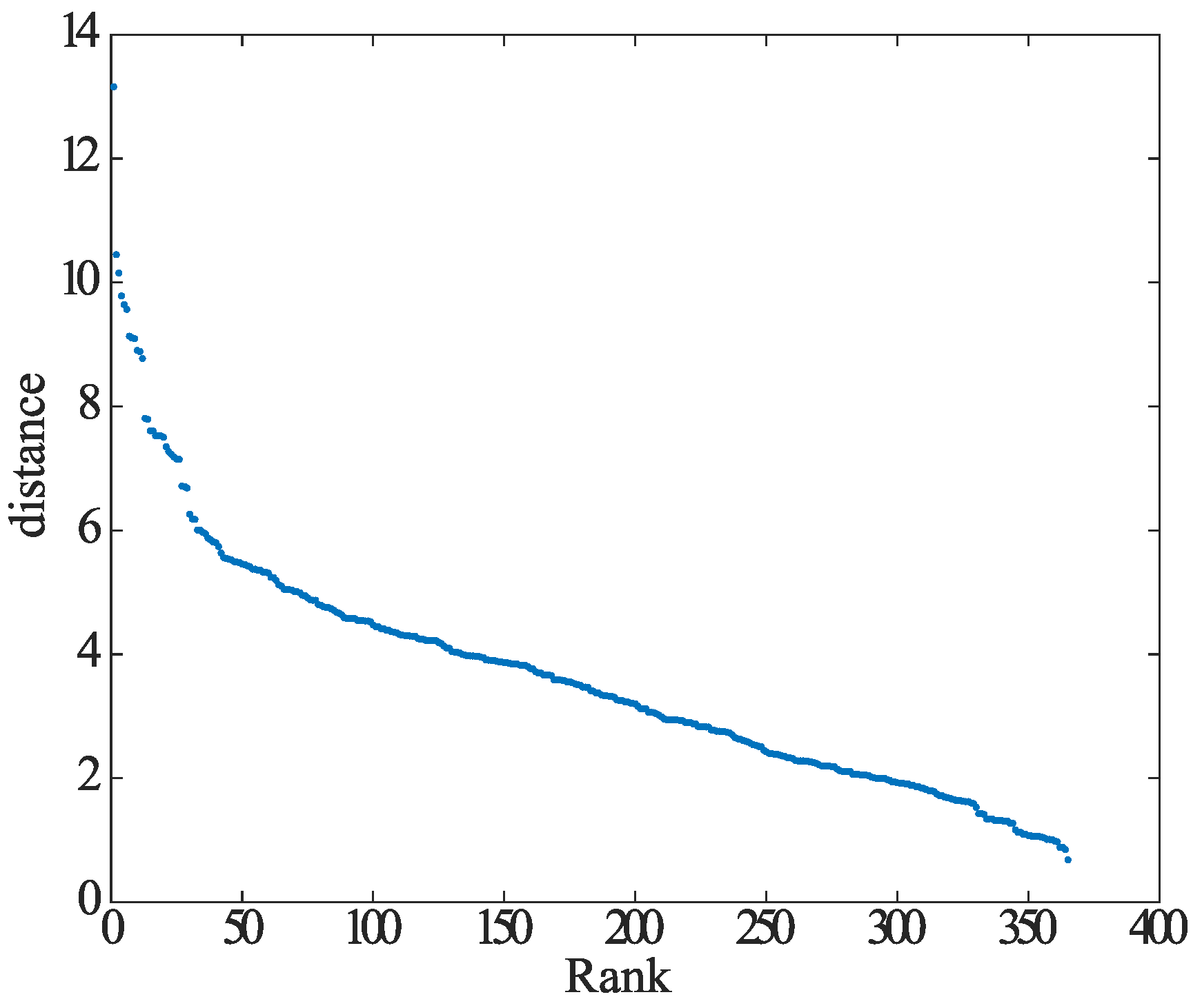
- The distance from each element to the kth element away is k-dist.
- The k-dist-mean is the average of the distances of each element to all elements contained within the radius k-dist.
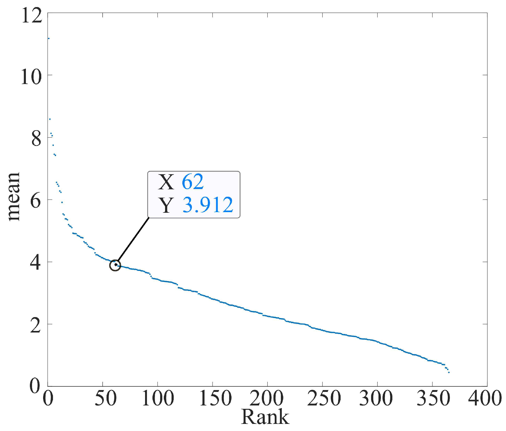
- Arrange the obtained k-dist-means in descending order.
- Find one point P that is the knee from the graph.
- The resulting k-dist value of point P is the radius , and the number of elements that the k-dist-mean of point P contains is MinPts.
2.4. Proposal Method
- Case 1: Clustering by improving k-dist plot
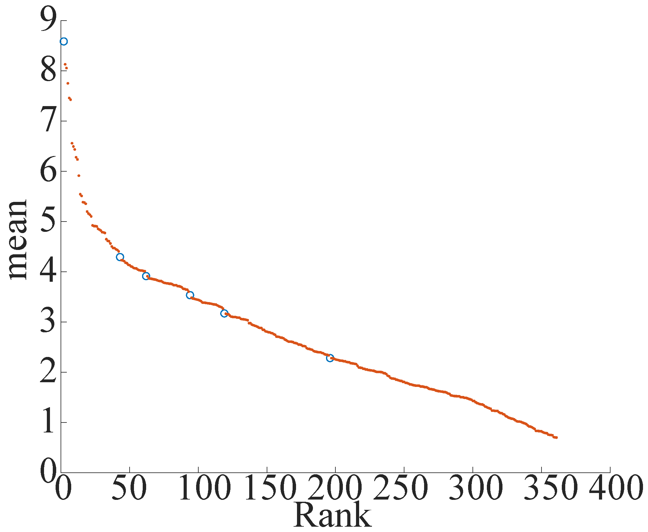
- Calculate the gradient between adjacent points of elements of the reordered k-dist-mean graph.
- From the graph, divide the elements into fixed intervals (10 equal parts in this paper) and find the average value of the gradient of the elements within the interval. The average slope for ranks 37–72 in Figure 5 is 0.0213.
- The element with a gradient value that is more prominent than the mean value (five times in this paper) is designated as the knee-point and stored in the knee-list. The gradient of the white circle for ranks 37–72 in Figure 5 was 0.1543, so it was stored in the knee-list as a Knee-Point.
- Here, for noise elimination, all the knee-points in the knee-list that have a prominent gradient ground (5 times in this paper) above the average of the gradient of the entire graph are eliminated. The average value of the overall slope in this study is 0.0303.
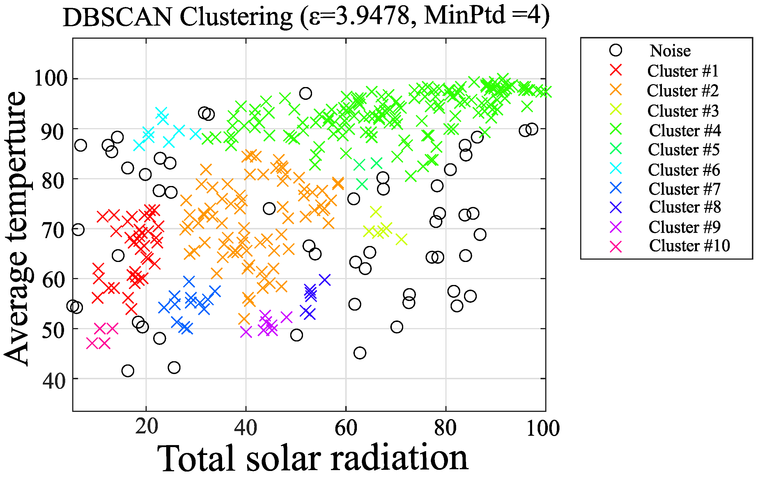
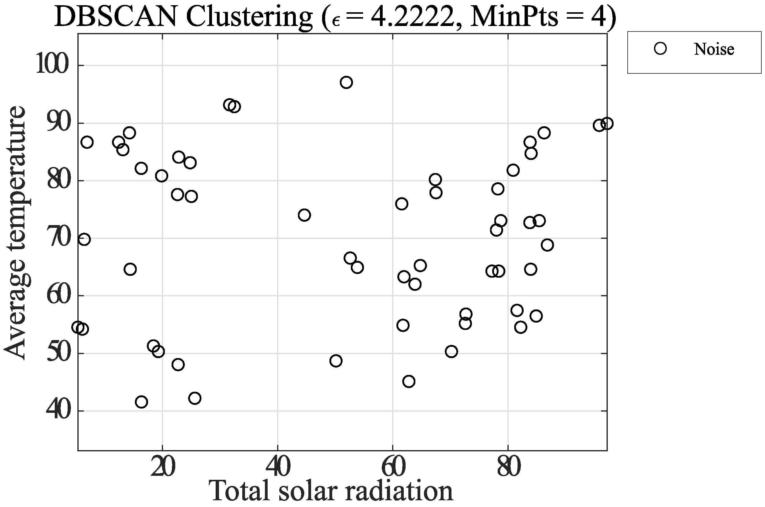
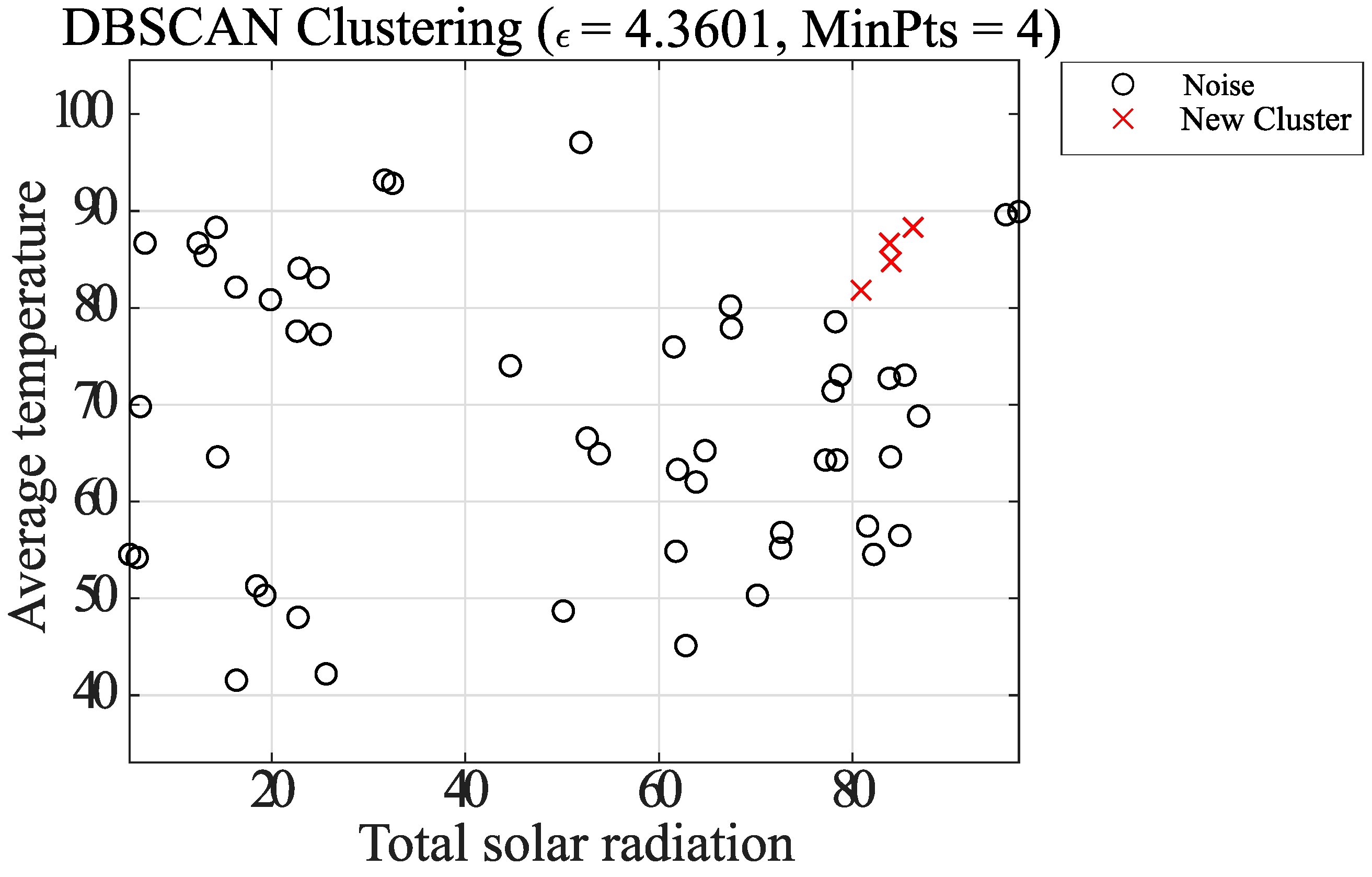
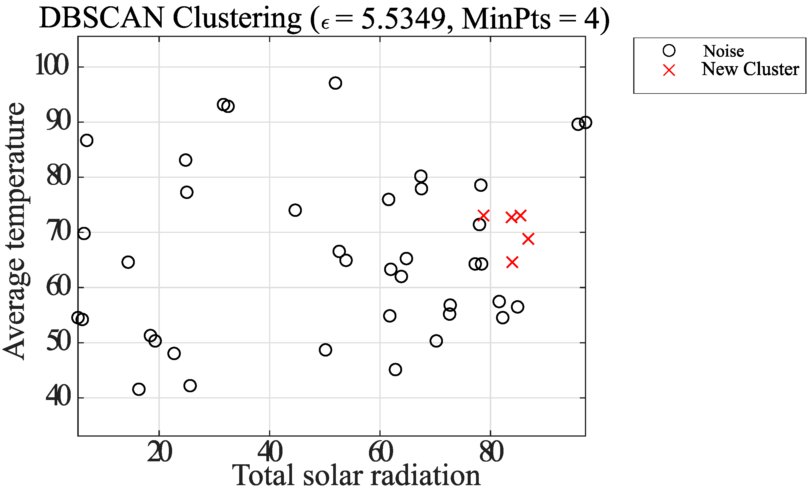
- Select the knee-point with the smallest k-dist value from the knee-list, calculate the radius and MinPts, and perform DBSCAN.
- All the elements assigned to clusters in the result obtained at this time are saved, and the saved elements are removed from the two-dimensional plane. Then, DBSCAN is performed on the next knee-point with a large k-dist as in step 5.
- Perform step 6 for all knee points in the knee list and finish clustering by adapting DBSCAN on all elements. Finally, the stored grouped elements and noise are shown in the same graph.
- Case 2: Clustering by combination of DBSCAN and k-means method
- Removal of noisy elements
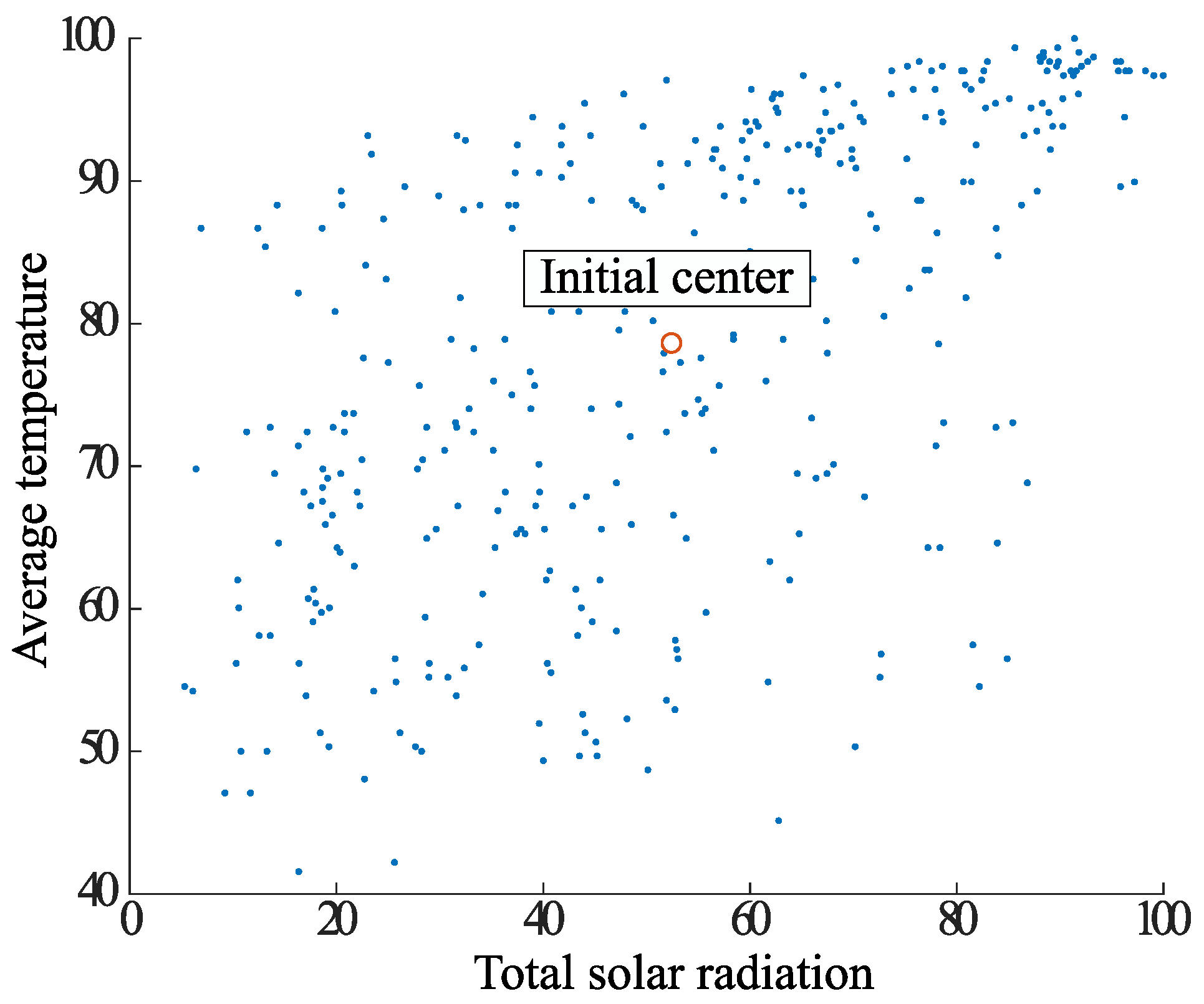
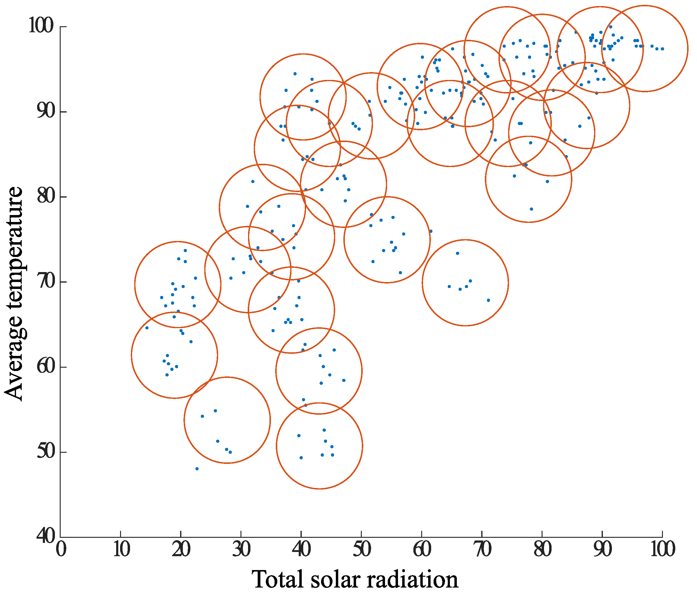
- Plot the points that are the centers of gravity of all the elements on the diagram, with P as the center of gravity.
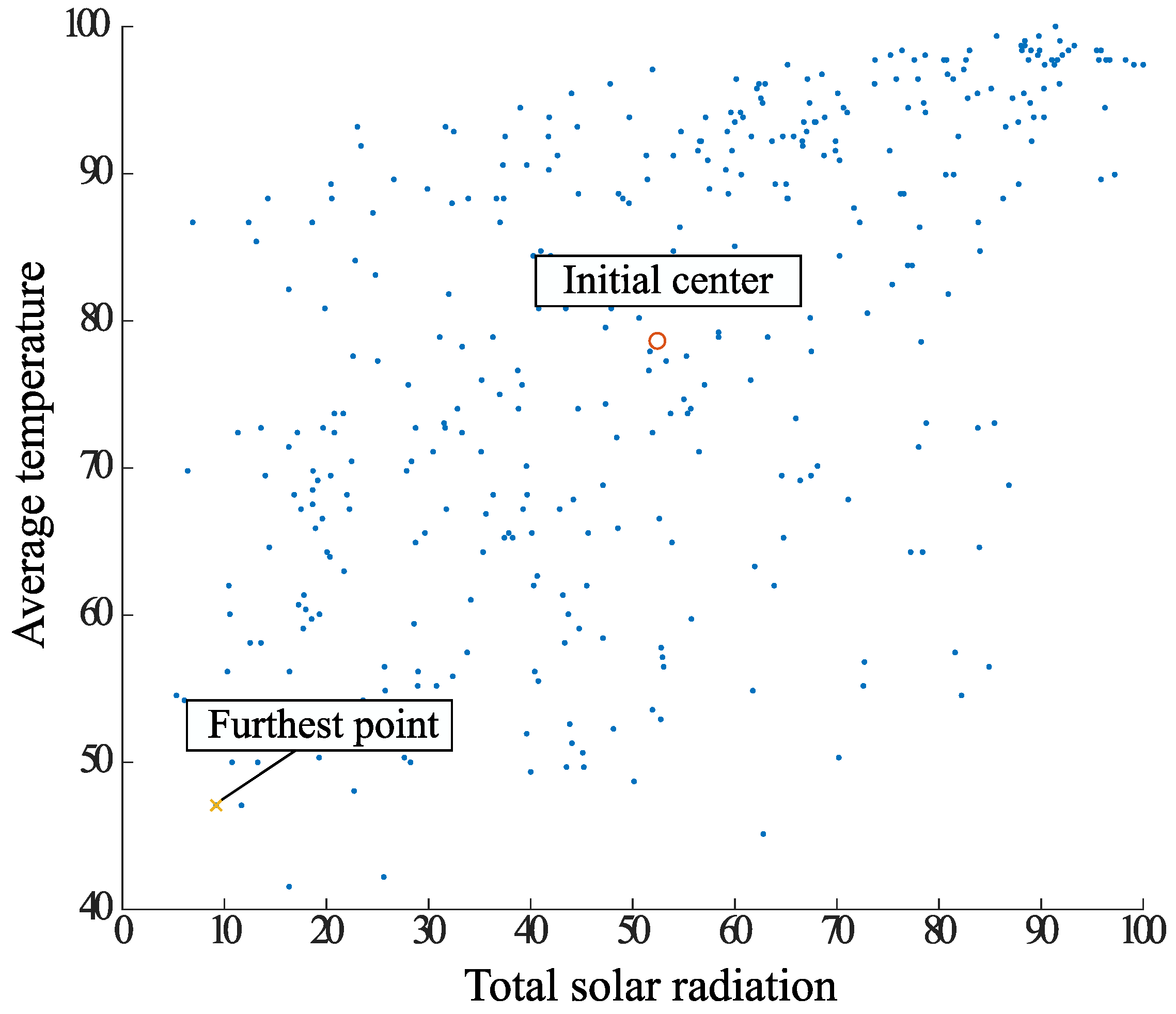
- Create a circle centered at point P that covers the entire element, and let r be its radius.
- The radius r is contracted, and the point S is the point of leakage from the circle.
- Consider a circle of radius with respect to S. Find the center of gravity of the elements contained in the circle and plot it on the diagram.
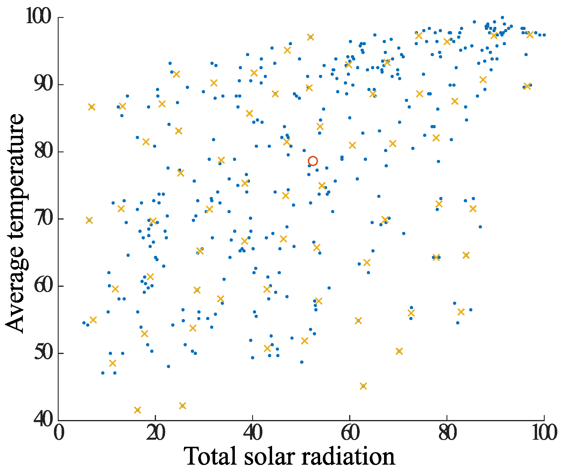
- Steps 3 to 4 are repeated until there are no more elements. The elements used in step 4 to calculate the center of gravity are excluded from the next step if they have been considered once.
- For every center of gravity obtained, a judgment is made as to whether it has Pts elements within a radius , and all elements within the circle of the center of gravity that do not satisfy the condition are considered noise.
- Classification of Elements
- 7.
- To classify the remaining centers of gravity and elements, the following method is used for grouping.
- (a)
- Focusing on the center of gravity farthest from the center of gravity P obtained in step 1, group together the elements contained within the radius of the center of gravity and make a new grouping.
- (b)
- Create a new center of gravity from the elements in the summarized group, and create a new group of elements contained within a radius centered on the center of gravity.
- (c)
- Repeat updating the center of gravity and groups as above, and save the groups when there are no more updates.
- (d)
- Next, the points away from the center of gravity P are grouped in the same way. At this time, elements that have been grouped once are not considered.
- 8.
- If groups have the same elements within the radius of the center of gravity of each other, they are considered as one group. In such a case, the group is considered to be a single group. A group is considered as a group with multiple centers of gravity.
- 9.
- Finally, clustering is performed on all groups using the k-means method. The number of clusters k is the number of centers of gravity that the group has. After updating the center of gravity with k-means, the clustering is finished.
Time Complexity
3. Formulation of the Optimization Problem
- objective functionwhere : the fuel cost of generator j at time k and : the starting cost of generator j at time k. The is given by the following equation.where : the output of generator j at time k, : the fuel cost coefficient of generator j.
- Constraints
- -
- Supply and demand balance constraints:Constraint that load demand and power supply at each bus bar must be equal.where : load demand on bus b at time k, : output of generator j on bus b at time k, : transmission line tidal flow on bus b at time k.
- -
- Generator output upper and lower limit constraints:The output of the generator must be within a certain range.where : minimum output of generator j, : maximum output of generator j.
- -
- Generator output change rate constraint:The rate of change of the generator output in one hour must be within a certain value.where : the maximum output change of generator j.
- -
- Power line tidal constraintsThe amount of transmission line tidal flow must be within a certain range.where : maximum capacity of the transmission line between busbars , : reactance of the transmission line between busbars , : transfer angle of busbars at time k.
- -
- Generator minimum run/stop time constraints:If the generator is started, it must not be stopped for the minimum operating time. Conversely, if the generator is stopped, it must not be started for the minimum time.where , : minimum operation and shutdown time of generator j, , : time to keep generator j stopped at time k.
- -
- Operating reserve capacity constraint:where : the operating reserve at time k busbar b.
- -
- Prediction error correspondence constraints:The following constraint equation is considered in the UC problem, which is a constraint to prevent changes in the start-up and shutdown states of generators determined in the pre-decision phase when errors in PV output occur within ±2 in the day’s operation plan.where D: load demand forecast, : PV output forecast, : standard deviation of PV output forecast error.
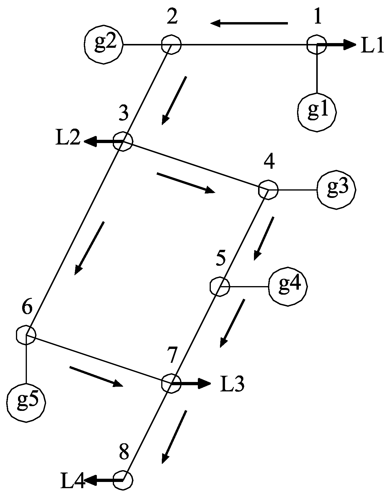
4. Power System Model
5. Simulation
5.1. Simulation Conditions
5.2. Simulation Results
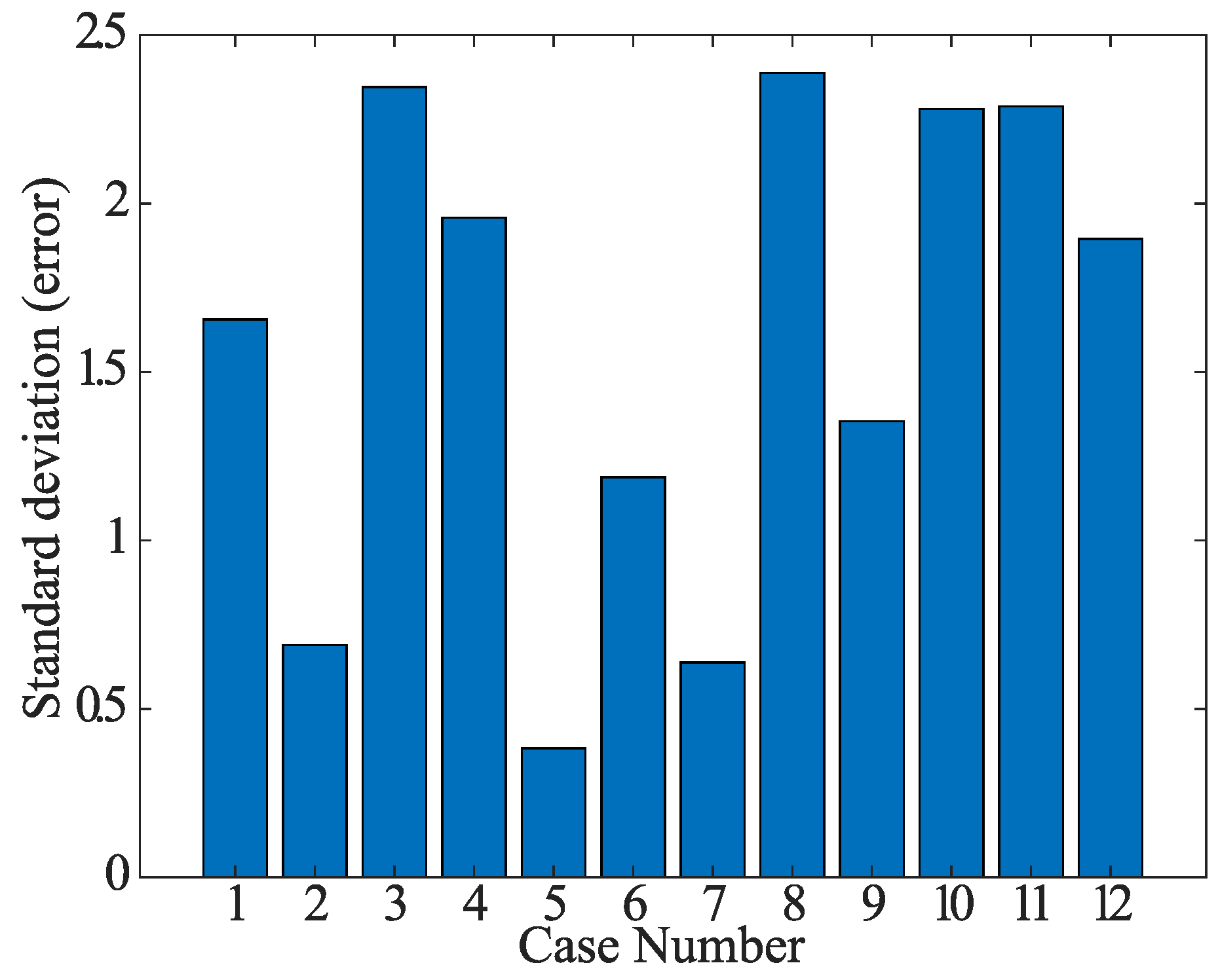
5.3. Analysis of Each Data
5.4. Simulation with Storage Batteries Installed
6. Conclusions
Author Contributions
Funding
Data Availability Statement
Conflicts of Interest
References
- Edmunds, R.; Davies, L.; Deane, P.; Pourkashanian, M. Thermal power plant operating regimes in future British power systems with increasing variable renewable penetration. Energy Conv. Manag. 2015, 105, 977–985. [Google Scholar] [CrossRef]
- Amrutha, A.A.; Balachandra, P.; Mathirajan, M. Role of targeted policies in mainstreaming renewable energy in a resource constrained electricity system: A case study of Karnataka electricity system in India. Energy Policy 2017, 106, 48–58. [Google Scholar] [CrossRef]
- Leonard, M.D.; Michaelides, E.E.; Michaelides, D.N. Substitution of coal power plants with renewable energy sources—Shift of the power demand and energy storage. Energy Convers. Manag. 2018, 164, 27–35. [Google Scholar] [CrossRef]
- Muralikrishnan, N.; Jebaraj, L.; Rajan, C.C.A. A Comprehensive Review on Etionary Optimization Techniques Applied for Unit Commitment Problem. IEEE Access 2020, 8, 132980–133014. [Google Scholar] [CrossRef]
- Li, X.; Zhai, Q.; Zhou, J.; Guan, X. A variable reduction method for large-scale unit commitment. IEEE Trans. Power Syst. 2020, 35, 261–272. [Google Scholar] [CrossRef]
- Guan, X.; Luh, P.B.; Yan, H.; Amalfi, J.A. An Optimization—Based Method for Unit Commitment. Electr. Power Energy Syst. 1992, 14, 9–17. [Google Scholar] [CrossRef]
- Howlader, H.O.R.; Sediqi, M.M.; Ibrahimi, A.M.; Senjyu, T. Optimal Thermal Unit Commitment for Solving Duck Curve Problem by Introducing CSP, PSH and Demand Response. IEEE Access 2018, 6, 4834–4844. [Google Scholar] [CrossRef]
- Zhu, Y.; Gao, H. Improved Binary Artificial Fish Swarm Algorithm and Fast Constraint Processing for Large Scale Unit Commitment. IEEE Access 2020, 8, 152081–152092. [Google Scholar] [CrossRef]
- Carrion, M.; Arroyo, J.M. A computationally efficient mixed–integer linear formulation for the thermal unit commitment problem. IEEE Trans. Power Syst. 2006, 21, 1371–1378. [Google Scholar] [CrossRef]
- Bragin, M.A.; Luh, P.B.; Yan, B.; Sun, X. A scalable solution methodology for mixed–integer linear programming problems arising in automation. IEEE Trans. Autom. Sci. Eng. 2019, 16, 531–541. [Google Scholar] [CrossRef]
- Viana, A.; PedroPedroso, J. A new MILP-based approach for unit commitment in power production planning. Electr. Power Energy Syst. 2013, 44, 997–1005. [Google Scholar] [CrossRef] [Green Version]
- Alemany, J.; Kasprzyk, L.; Magnago, F. Effects of binary variables in mixed integer linear programming based unit commitment in large–scale electricity markets. Electr. Power Syst. Res. 2018, 160, 429–438. [Google Scholar] [CrossRef]
- Balasubramanian, S.; Balachandra, P. Characterising electricity demand through load curve clustering: A case of Karnataka electricity system in India. Comput. Chem. Eng. 2021, 150, 107316. [Google Scholar] [CrossRef]
- Marton, C.H.; Elkamel, A.; Duever, T.A. An order-specific clustering algorithm for the determination of representative demand curves. Comput. Chem. Eng. 2008, 32, 1365–1372. [Google Scholar] [CrossRef]
- Ibs-von Seht, M. Detection and identification of seismic signals recorded at Krakatau ano (Indonesia) using artificial neural networks. J. Anology Geotherm. Res. 2008, 178, 448–456. [Google Scholar] [CrossRef]
- Lei, M.; Shiyan, L.; Chuanwen, J.; Hongling, L.; Yan, Z. A review on the forecasting of wind speed and generated power. Renew. Sustain. Energy Rev. 2009, 13, 915–920. [Google Scholar] [CrossRef]
- MacQueen, J.B. Some Methods for Classification and Analysis of Multivariate Observation. In Proceedings of the Berkeley Symposium on Mathematical Statistics and Probability 5.1, Berkeley, CA, USA, 7 January 1967; pp. 281–297. [Google Scholar]
- Kaur, P.; Goyal, M.; Lu, J. Data mining driven agents for predicting online auction’s end price. In Proceedings of the 2011 IEEE Symposium on Computational Intelligence and Data Mining (CIDM), Paris, France, 11–15 April 2011; p. 141. [Google Scholar]
- Understanding Clustering with the K-Means Algorithm in Machine Learning: (With Examples). Available online: https://www.analyticsvidhya.com/blog/2021/11/understanding-k-means-clustering-in-machine-learningwith-examples/ (accessed on 20 January 2023).
- Luo, X.; Zhu, X.; Lim, E.G. A parametric bootstrap algorithm for cluster number determination of load pattern categorization. Energy 2019, 180, 50–60. [Google Scholar] [CrossRef]
- Battaglia, O.R.; Paola, B.D.; Fazio, C. A New Approach to Investigate Students’ Behavior by Using Cluster Analysis as an Unsupervised Methodology in the Field of Education. Appl. Math. 2016, 7, 141–147. [Google Scholar] [CrossRef] [Green Version]
- Nobis, M.; Schmitt, C.; Schemm, R.; Schnettler, A. Pan-European CVaR-Constrained Stochastic Unit Commitment in Day-Ahead and Intraday Electricity Markets. Energies 2020, 13, 2339. [Google Scholar] [CrossRef]
- Ocampo, E.; Huang, Y.; Kuo, C.-C. Feasible Reserve in Day-Ahead Unit Commitment Using Scenario-Based Optimization. Energies 2020, 13, 5239. [Google Scholar] [CrossRef]
- Heuberger, C.F.; Staffell, I.; Shah, N.; Mac Dowell, N. A systems approach to quantifying the value of power generation and energy storage technologies in future electricity networks. Comput. Chem. Eng. 2017, 107, 247–256. [Google Scholar] [CrossRef]
- Khan, K.; Rehman, S.U.; Aziz, K.; Fong, S.; Sarasvady, S. DBSCAN: Past, present and future. In Proceedings of the ICADIWT, Bangalore, India, 17–19 February 2014; pp. 232–238. [Google Scholar]
- Ester, M.; Sander, H.K.J.; Xu, X. A density-based algorithm for discovering clusters in large spatial databases. In Proceedings of the KDD ’96 Proceeding of the Second International Conference on Knowledge Discovery and Data Mining, Oregon, Portland, 2–4 August 1996; pp. 226–231. [Google Scholar]
- Gaonkar, M.N.; Sawant, K. Auto Eps DBSCAN: DBSCAN with Eps automatic for large dataset. Int. J. Adv. Comput. Theory Eng. 2013, 2, 11–16. [Google Scholar]
- Japan Meteorological Agency. Available online: https://www.data.jma.go.jp/obd/stats/etrn/index.php (accessed on 20 January 2023).
- Okinawa Electric Power|Electricity Forecast. Available online: https://www.okiden.co.jp/denki2/dl (accessed on 20 January 2023).
- Pandi, H.; Wang, Y.; Qiu, T.; Dvorkin, Y.; Kirschen, D.S. Near-Optimal Method for Siting and Sizing of Distributed Storage in a Transmission Network. IEEE Trans. Power Syst. 2015, 30, 2288–2300. [Google Scholar]
- Aoyagi, H.; Isomura, R.; Mandal, P.; Krishna, N.; Senjyu, T.; Takahashi, A.H. Optimum Capacity and Placement of Storage Batteries Considering Photoaics. Sustainability 2019, 11, 2556. [Google Scholar] [CrossRef] [Green Version]
- Blanco, R.F.; Dvorkin, Y.; Xu, B.; Wang, Y.; Kirsche, D.N. Optimal energy storage siting and sizing: A WECC case study. In Proceedings of the 2017 IEEE Power & Energy Society General Meeting, Chicago, IL, USA, 17 July 2017; p. 1. [Google Scholar]
- Çunkaş, M.; Altun, A.A. Long Term Electricity Demand Forecasting in Turkey Using Artificial Neural Networks. Energy Sources Part Econ. Plan. Policy 2010, 5, 279–289. [Google Scholar] [CrossRef]


| Data Element |
|---|
| 1. Average humidity [%] |
| 2. Load demand [MW] |
| 3. Total precipitation [mm] |
| 4. Total solar radiation [Mj/m] |
| 5. Maximum temperature [℃] |
| 6. Average temperature [℃] |
| 7. Minimum temperature [℃] |
| 8. Load maximum time [hour] |
| 9. Minimum load time [hour] |
| 10. Maximum wind speed [m/s] |
| 11. Average wind speed [m/s] |
| 12. Weekdays, weekends, and holidays |
| P | P | P | A | B | C | SUC | T | ||
|---|---|---|---|---|---|---|---|---|---|
| [MW] | [MW] | [MW] | [JNY] | [JNY/MWh] | [JNY/MWh] | [¥] | [h] | ||
| g1-1(Coal) | 220 | 84 | 44 | 80,000 | 4000 | 0.4 | 1,100,000 | 8 | |
| g1-2(Coal) | 220 | 84 | 44 | 80,000 | 4000 | 0.4 | 1,100,000 | 8 | |
| g2-1(oil) | 125 | 103 | 62.5 | 632,000 | 9200 | 2.0 | 375,000 | 6 | |
| g2-2(oil) | 103 | 50 | 51.5 | 632,000 | 9200 | 2.0 | 309,000 | 6 | |
| g3-1(Coal) | 156 | 60 | 31.2 | 80,000 | 4000 | 0.4 | 780,000 | 6 | |
| g3-2(Coal) | 156 | 60 | 31.2 | 80,000 | 4000 | 0.4 | 780,000 | 6 | |
| g4-1(LNG) | 251 | 122 | 84 | 132,000 | 4400 | 5.0 | 753,000 | 8 | |
| g4-2(LNG) | 251 | 122 | 84 | 132,000 | 4400 | 5.0 | 753,000 | 8 | |
| g4-3(LNG) | 35 | 17 | 35 | 132,000 | 4400 | 5.0 | 105,000 | 4 | |
| g5-1(oil) | 125 | 60 | 62.5 | 632,000 | 9200 | 2.1 | 375,000 | 6 | |
| g5-2(oil) | 60 | 30 | 30 | 632,000 | 9200 | 2.1 | 180.000 | 4 | |
| g5-3(oil) | 103 | 55 | 51.5 | 632,000 | 9200 | 2.1 | 309,000 | 6 | |
| Bus Line | Equipment Capacity [MW] | Operating Capacity [MW] | Available Capacity [MW] |
|---|---|---|---|
| 1-2 | 1208 | 1032 | 177 |
| 2-3 | 998 | 650 | 73 |
| 2-4 | 1208 | 650 | 286 |
| 3-4 | 758 | 432 | 157 |
| 4-5 | 1208 | 650 | 192 |
| 3-6 | 810 | 574 | 102 |
| 5-7 | 1150 | 650 | 133 |
| 6-7 | 596 | 340 | 110 |
| 7-8 | 520 | 260 | 54 |
| Error [%] | Simulation Time [s] | Number of Clusters | Time Error [%] | |
|---|---|---|---|---|
| One year operation | - | 9689 | - | 100 |
| DBSCAN (data4 and 6) | 2.7 | 62 | 4 | 0.63 |
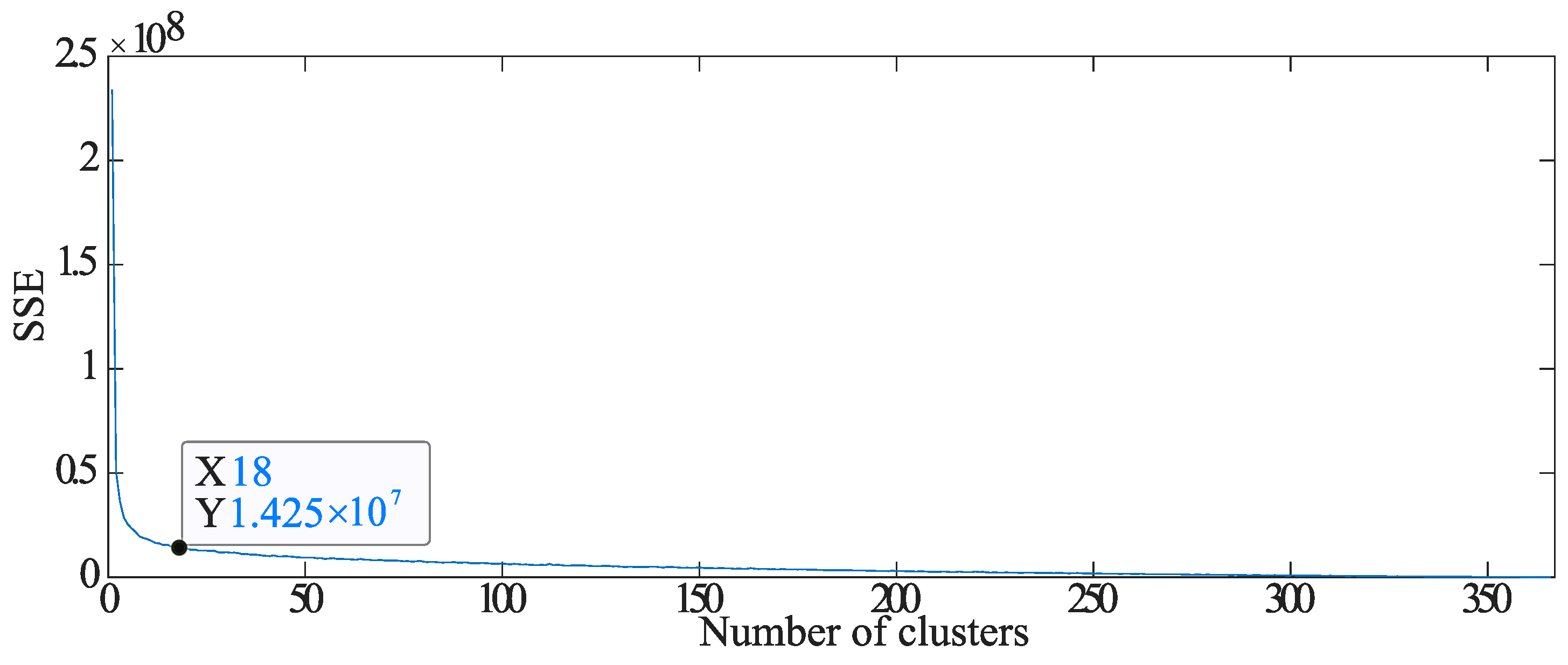
| k-means | 1.3 | 356 | 18 | 3.6 |
| Case 1 (data2 and 12) | 1.2 | 182 | 12 | 1.9 |
| Case 2 (data6 and 9) | 0.5 | 265 | 18 | 2.7 |
| Bus Number | 1 | 2 | 3 | 4 | 5 | 6 | 7 | 8 | Total |
|---|---|---|---|---|---|---|---|---|---|
| Base case | 0 | 0 | 2 | 0 | 0 | 0 | 44 | 39 | 85 |
| Proposed 2 | 0 | 0 | 0 | 2 | 0 | 2 | 53 | 23 | 80 |
| [Million JNY] | ESS Cost | Operation Cost | Total Cost |
|---|---|---|---|
| Base case | 10.88 | 386.7 | 397.6 |
| Proposed2 | 10.24 | 388.9 | 399.0 |
Disclaimer/Publisher’s Note: The statements, opinions and data contained in all publications are solely those of the individual author(s) and contributor(s) and not of MDPI and/or the editor(s). MDPI and/or the editor(s) disclaim responsibility for any injury to people or property resulting from any ideas, methods, instructions or products referred to in the content. |
© 2023 by the authors. Licensee MDPI, Basel, Switzerland. This article is an open access article distributed under the terms and conditions of the Creative Commons Attribution (CC BY) license (https://creativecommons.org/licenses/by/4.0/).
Share and Cite
Tanigawa, Y.; Krishnan, N.; Oomine, E.; Yona, A.; Takahashi, H.; Senjyu, T. Clustering Method for Load Demand to Shorten the Time of Annual Simulation. Energies 2023, 16, 2264. https://doi.org/10.3390/en16052264
Tanigawa Y, Krishnan N, Oomine E, Yona A, Takahashi H, Senjyu T. Clustering Method for Load Demand to Shorten the Time of Annual Simulation. Energies. 2023; 16(5):2264. https://doi.org/10.3390/en16052264
Chicago/Turabian StyleTanigawa, Yuya, Narayanan Krishnan, Eitaro Oomine, Atushi Yona, Hiroshi Takahashi, and Tomonobu Senjyu. 2023. "Clustering Method for Load Demand to Shorten the Time of Annual Simulation" Energies 16, no. 5: 2264. https://doi.org/10.3390/en16052264