
Generalised Isentropic Relations in Thermodynamics

Department of Process & Energy, Delft University of Technology, 2628 CD Delft, The Netherlands
*
Author to whom correspondence should be addressed.
†
A former researcher in Department of Process & Energy TU Delft.
Energies 2023, 16(5), 2281; https://doi.org/10.3390/en16052281
Submission received: 21 November 2022
/
Revised: 9 February 2023
/
Accepted: 20 February 2023
/
Published: 27 February 2023
(This article belongs to the Section J2: Thermodynamics)
Abstract
:Isentropic processes in thermodynamics are fundamental to our understanding of numerous physical phenomena across different scientific and engineering fields. They provide a theoretical reference case for the evaluation of real thermodynamic processes and observations. Yet, as analytical relations for isentropic transformations in gas dynamics are limited to ideal gases, the inability to analytically describe isentropic processes for non-ideal gases is a fundamental shortcoming. This work presents generalised isentropic relations in thermodynamics based on the work by Kouremenos et al., where three isentropic exponents , and are introduced to replace the ideal gas isentropic exponent to incorporate the departure from the non-ideal gas behaviour. The general applicability of the generalised isentropic relations is presented by exploring its connections to existing isentropic models for ideal gases and incompressible liquids. Generalised formulations for the speed of sound, the Bernoulli equation, compressible isentropic flow transformations, and isentropic work are presented thereafter, connecting previously disjoint theories for gases and liquids. Lastly, the generalised expressions are demonstrated for practical engineering examples, and their accuracy is discussed.
1. Introduction
Isentropic processes describe idealized processes without irreversibilities such as friction or heat losses and are therefore used as a theoretical reference case for the evaluation of real thermodynamic processes and observations. For this reason, isentropic relations are encountered in many fields of science and engineering applications. In fluid dynamics, where flows are approximated as isentropic flows outside the viscous boundary layer, the isentropic relations are an intrinsic part of modelling fluid compressibility and are, therefore, an underlying assumption in aerodynamics. In energy engineering, the isentropic relations find their way into evaluating the isentropic work of gas compression and expansion systems and are also fundamental to turbo-machinery design. Driven by increasing energy and fuel efficiency, state-of-art energy conversion systems, such as the supercritical CO cycle [1,2,3], Organic Rankine Cycles [4], and high-pressure industrial heat pumps [5], seek to exploit the non-ideal behaviour of unconventional working fluids where the ideal gas approximation is no longer valid. As the ideal gas equation is used to relate isentropic transformations, their application is limited to ideal gases only. The conventional classification between “ideal” and “non-ideal” is distinctive for the apparent lacking means to conveniently describe isentropic processes in the general sense.
Where isentropic processes for ideal gases are conveniently modelled by the isentropic exponent —the often assumed constant ratio of the specific isobaric and isochoric heat capacities and —our capabilities are limited in the general case, where engineers and scientists are forced to resort to thermodynamic libraries, look-up tables, and equations of state of (semi)-empirical nature. Although this may not be a problem with today’s computing power and access to powerful (open-source) libraries, such as CoolProp [6] and RefProp [7], the lacking ability to describe isentropic processes in a general way is a gap in our understanding of thermodynamics, as isentropic transformations under the ideal gas model cannot simply be projected on non-ideal gas applications as their gas-dynamic behaviour is vastly different.
In a series of papers published in the 1980s, on which this work is based, Kouremenos et al. proposed a set of generalised isentropic relations to model isentropic processes in a general way [8,9,10]. They introduced three isentropic exponents to replace the adiabatic coefficient , based on the mathematical argument that the form of a generalised model should adhere to its ideal gas counterpart. Compressibility effects and departure from the ideal gas behaviour are then included in three alternative isentropic exponents. Although their derivation of the general isentropic model appeared successful, they did not pursue to extend their analysis to existing isentropic transformations, but instead performed empirical evaluations of the isentropic exponents using an equations of state [9,11]. A similar model was later proposed by Baltadijev, who made efforts to derive additional isentropic flow relations [12]. Nederstigt [13] further extended this approach to develop generalised isentropic relations for several process quantities. Recently, the non-ideal gas isentropic exponents also found their way into the field of computational fluid dynamics [14].
This work seeks to introduce the generalised isentropic relations proposed by Kouremenos et al. to a broader audience and to complete the analytical framework by addressing previously unexplored connections with existing isentropic models for ideal gases and liquids—connecting previously disjoint theories for speed of sound, isentropic flows, and isentropic work between gases and liquids. Finally, the applicability of the generalised isentropic relations is demonstrated for practical engineering examples, and their accuracy is discussed.
2. Isentropic Exponents for the Real Gas Thermodynamic Region
2.1. Generalised Isentropic Relations
First, the generalised isentropic relations proposed by Kouremenos et al. [8,9,10] are presented. The model is based on the isentropic relations of ideal gases where the ratio of the specific heats is replaced by exponents , and . The subscripts refer to the pressure–volume, temperature–volume, and pressure–temperature isentrope governed by each of the exponents, respectively, summarised as
where P is the pressure, v—the specific volume, and T—the temperature. Consequently, the pressure ratio, temperature ratio, and density ratios in any isentropic transformation can be related by
where subscripts 1 and 2 refer to the respective thermodynamic states along an isentrope.
The generalised isentropic exponents are then to be expressed in terms of other thermodynamic state variables, which will be demonstrated to be a function of the specific heat capacities and partial derivatives in pressure, volume, and temperature. The derivation of exponent is shown here as an example [13].
Let the entropy s be defined as a function of pressure and temperature, such that . Consequently, the change in entropy can be expressed as the exact differential
where for an isentropic process. Rearranging the derivatives yields
The left-hand side of Equation (4) can be evaluated by differentiation of the assumed isentropic pressure–temperature relation, Equation (1c), yielding
The right-hand side of Equation (4) can be transformed using Maxwell’s relations
where .
Finally, equating Equations (5) and (6), an expression for is obtained in terms of pressure P, the isobaric specific heat capacity , and the partial derivative , given as
The exponents and for the temperature-volume and pressure-volume isentrope can be derived in a similar fashion from Equations (1a) and (1b) [13]. Together, the three generalised isentropic relations can be summarized as
where is the thermal expansion coefficient and —the isothermal compressibility factor [12].
As, according to Gibbs’ phase rule, the thermodynamic state of a (pseudo)-pure single-phase substance is determined by two state variables, only two of the generalised isentropic exponents are independent. Following from Equations (8a)–(8c), the thermal expansion coefficient and isothermal compressibility factor can be expressed in terms of the exponents and as
Moreover, a reciprocity can be observed between the exponents , , and through their partial derivatives, related by the triple product rule
The isentropic exponents are thus related by [8]
2.2. Limits of the Generalised Isentropic Exponents for Ideal Gases and Incompressible Liquids
Thus far, no assumptions have been made on the thermodynamic state in the derivation of the generalised isentropic relations, nor has any equation of state been introduced to relate pressure, temperature, density, and fluid compressibility. In general, the term real gas itself is ambiguous to any thermodynamic state and broadly covers the entire range from dilute gases to dense gases and compressible liquids.
Regardless of the equation of state used, the generalised isentropic relations must agree with existing isentropic models for liquids and ideal gases. In the case of liquids, that means that the isentropic relations Equations (8a)–(8c) should adopt the form of the incompressible fluid model, accounting for negligible changes in density with changing pressure under constant entropy. Note, for a van der Waals fluid, the incompressible limit is reached as the specific volume , with being the volume at the thermodynamic liquid-vapour critical point [13]. On the other hand, for ideal gases, the generalised isentropic relations should reduce to the familiar isentropic expressions for ideal gases. The connections to these models will now be discussed.
Ideal gas region: In the case of ideal gases, it can be shown that the generalised isentropic exponents reduce to the adiabatic coefficient , defined as the ratio of the specific heats /. Evaluating the partial derivatives in Equations (8a)–(8c), using the ideal gas model gives [13],
where the universal gas constant R is related to the specific heat capacities by in the ideal gas case. Consequently, the real gas exponents , , and are shown to be identical to their ideal gas counterparts
This is ultimately a mathematical requirement by adopting the ideal gas solution as the starting point of the derivation for the non-ideal isentropic exponents.
Liquid phase region: At the limit of an incompressible fluid model, the changes in fluid density with pressure are negligible. Consequently, , , and the exponent approaches infinity, see Equation (8a). Likewise, from Equation (8b), we find that as , and the exponent becomes infinite as well. Note, the thermal expansion coefficient . Subsequently, eliminating using the relation between the specific heat capacities and in Equation (8c), gives
The right-hand side of Equation (8c) can be shown to go to zero. Consequently, we find that for incompressible substances. The incompressible limits can therefore be summarized as
for which the generalised isentropic exponents become
Liquid–vapour coexistence region: As the specific heat capacities and are undefined in the two-phase region, neither are the real isentropic exponents , , and . It follows from here that the non-ideal isentropic exponents are only generally defined for single-phase substances.
Real gas region: The conditions for thermal and mechanical stability of a single-phase substance require that the isochoric specific heat capacity and the isothermal compressibility [15,16]. The latter condition implies that the partial derivative . By reciprocity between the partial derivatives with respect to pressure, temperature, and density in Equation (10), the conditions for mechanical stability can be expressed as [15,16]
As neither the specific heat capacities, nor the pressure, temperature, and specific volume can be negative, combining the inequalities in Equation (17) with Equations (8a)–(8c), it can be shown that
for single-phase substances.
A notable consequence of Equation (18), compared to the isentropic exponent for ideal gases, is that values of are permissible under the conditions for thermal and mechanical stability for single-phase substances. For instance, pentane shows a region where , as shown in Figure 1c. This gives new characteristics to isentropic transformations derived from .
The value of is, in fact, directly related to the fundamental derivative of gas dynamics , which is a non-dimensional quantity that governs the dynamic behaviour of gases. The fundamental derivative of gas dynamics is defined as the derivative of the speed of sound with respect to volume at constant entropy, or alternatively, the second derivative—or curvature—of the pressure–volume isentrope, expressed as [17,18]
The isentropic relations Equations (8a)–(8c) are hyperbolic functions that describe the isentropes in the pressure–volume, temperature–volume, and pressure–temperature plane. Their shape—and hence curvature—along any point of the isentrope is governed by the local value of the isentropic exponents, which are continuously varying functions along the isentrope. In the case of the fundamental derivative, substitution of Equation (8a) yields [13,19]
where the derivative is small compared to the first term in Equation (20) and may be omitted, Equation (20) is approximated by [13], equivalent to the value of for ideal gases, [17,18].
As non-classical behaviour is observed in dense gasses for [17], and cannot be negative, non-classical behaviour gas behaviour can only occur where the derivative term in Equation (20) is larger than .
The theoretical limits of the real isentropic relations are summarized in Table 1.
2.3. Isentropic Exponents Plotted in the Pv-Plane for Water, Carbon Dioxide, and Pentane
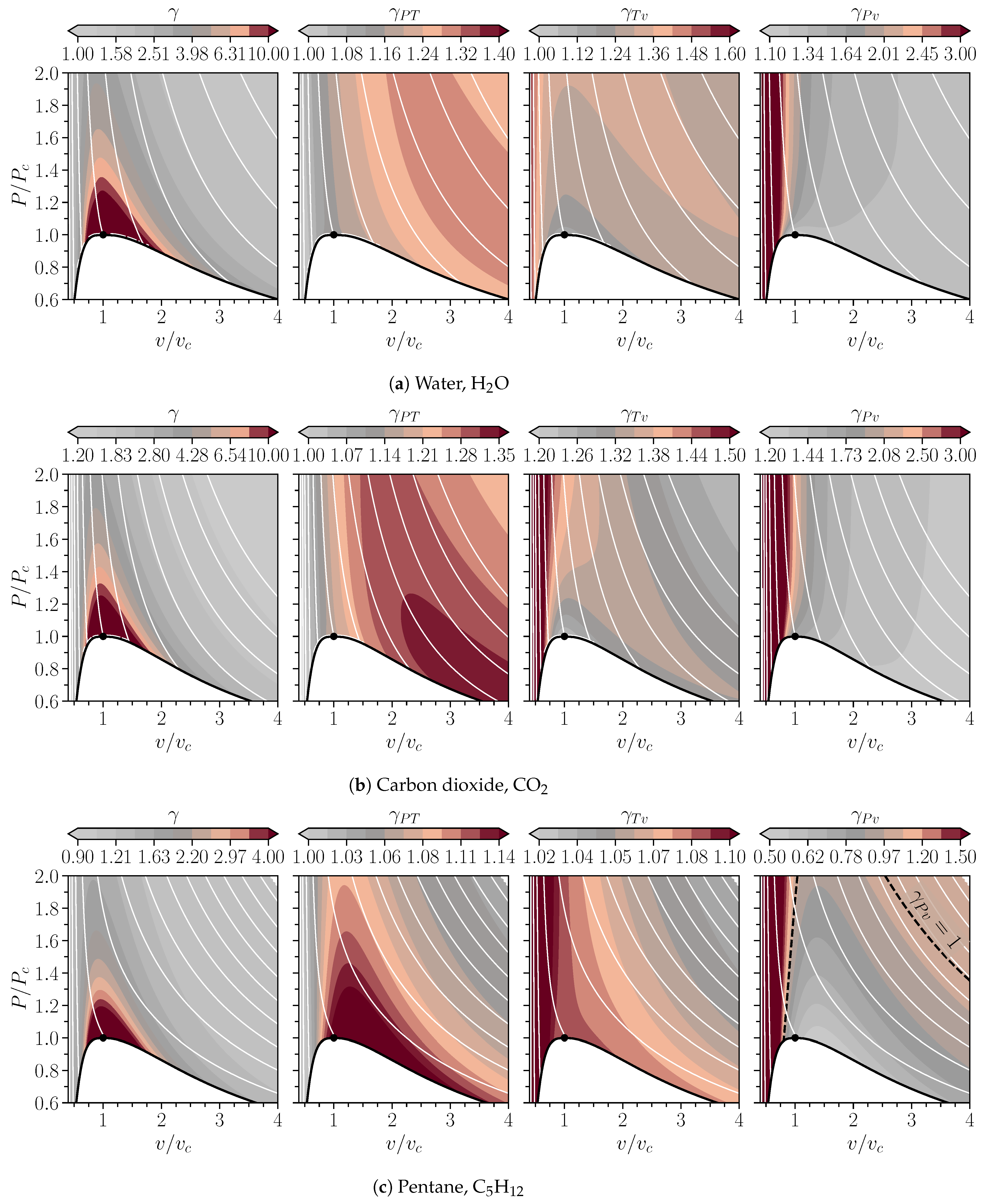
Figure 1 shows the specific heat ratio and the three generalised isentropic exponents for water, carbon dioxide, and pentane in the -plane obtained with RefProp version 10.0 [7]. The corresponding equations of state are given in refs. [20,21]. The three substances were chosen due to their many practical applications in the field of engineering and due to their difference in molecular size, complexity, and polarity.
First of all, the value of the ideal gas exponent is of a similar order of magnitude between the gaseous and liquid regions in Figure 1 for all three substances. Only around the critical point, a rise in the value of is seen due to the increase of the isobaric heat capacity around that point.
Comparing the generalised isentropic exponents, demonstrates the highest degree of variation, steeply increasing in value beyond the critical point for increasingly higher densities in the liquid region, ultimately approaching infinity. Though also tends to infinity for high densities, it quickly drops off, showing a milder progression in value change with decreasing density into the gaseous region. Exponent shows a smaller variation throughout the -plane, ranging from unity for high densities in the liquid region to the ratio of the specific heats for ideal gases.
Between the three fluids, it is observed that HO and CO—with a lower molecular complexity—show a stronger variation of all three the isentropic exponents with respect to pentane, for which variations are fewer.
The most notable difference between the three substances is the presence of a region where of pentane round the liquid–vapour coexistence region. Pentane has a dry liquid–vapour dome, where the concave shape of the vapour line results in dry expansion. The ratio of the specific heats has been found to control the skewness of the liquid–vapour dome in other research [22]. Whilst evaluating the contours of the isentropic exponents for various substances with RefProp, fluids with similar dry liquid–vapour domes were also found to possess a region where .
3. Generalised Speed of Sound, Isentropic Flows Transformations, and Isentropic Work
The generalised isentropic exponents are now used to derive generalised isentropic relations for practical engineering applications, such as the speed of sounds and isentropic flows through nozzles, compressors, and turbine stages.
3.1. Generalised Speed of Sound in Fluids
The speed of sound is defined as [25]
where is the density of the substance. Using the isentropic pressure–volume relation for real gases, Equation (8a), an expression for the speed of sound can be derived in terms of the exponent . The speed of sound is then given as [26,27]
Here, the benefit of adhering to the ideal gas notation for the isentropic relations becomes apparent as the departure from ideal gas conditions in Equation (22) is conveniently included in the exponent without losing the familiarity of the ideal gas notation.
In the case of liquids, the speed of sound is related to the bulk modulus —a measure for the elasticity of the fluid—known as the Newton–Laplace equation [28,29]
The bulk modulus of ideal gases is related to the ratio of the specific heats and the pressure through [25,28]. In its generalised form, the bulk modulus is related to the isentropic exponent through
Between gasses and liquids, the isentropic bulk modulus varies several orders of magnitude, typically ranging from kilopascals to megapascals for gases, to the order of gigapascals in the case of liquids. We can now relate this to the value of , which between gases and liquids of equal pressure is demonstrated in Figure 1 and Table 1 to change several orders of magnitude between gases and liquids as the derivative becomes large due to small fluid compressibility.
3.2. Isentropic Transformations for Non-Ideal Compressible Isentropic Flows
The generalised isentropic exponents are now used to derive transformations for non-ideal isentropic fluid flows from the fundamental conservation laws of mass, momentum, and energy. Though their derivation is similar to the ideal gas case, a different approach must be followed as, unlike ideal gases, the total enthalpy can no longer be related to the temperature using constant specific heats only. We start with the energy equation of a steady one-dimensional adiabatic flow [25]
where u the velocity, g—the gravitational constant, and —the change in elevation of the flow volume. In the case of ideal gases, the change in enthalpy may be directly related to the change in temperature using . In the general case, the change in enthalpy can be expressed in terms of pressure and the specific volume as , or alternatively, as , where is the fluid density. Substituting the latter in Equation (25), we obtain
Although it is possible to use the differential form of the Bernoulli equation to study isentropic transformations, it is more convenient to integrate Equation (26) for direct calculations. However, certain assumptions must be made to integrate in Equation (26). Assuming that is constant and that , the integration can be performed using the pressure–volume isentropic relation, Equation (8a), to give
Note that for certain cases, may be less than 1, e.g., as shown in Figure 1c. Therefore, it is possible for isentropic transformations to obtain , such that the right-hand side of (27) becomes singular. It is possible to integrate Equation (26) but this case will not be considered separately herein.
The generalised form of the Bernoulli equation for non-ideal fluid flows is then
which is applicable for the entire single-phase region for stable substances where . The ideal gas form of the Bernoulli equation is easily recognized, for which reduces to the adiabatic coefficient , as demonstrated in Equation (12). In the case of liquids, becomes large due to fluid incompressibility, and consequently , such that Equation (28) reduces to the classic form of the Bernoulli equation for incompressible fluid flows.
With the generalised Bernoulli equation for gases and liquids, the local flow properties can be related to the upstream fluid at rest as a reference state of the flow, with and denoting the stagnation pressure and density. Ignoring body forces, the downstream flow can be related to the stagnation conditions by
where a constant value of is assumed throughout the isentropic flow field.
The velocity can be expressed in terms of local Mach number as with as the local speed of sound Equation (22). Gathering the pressure terms on the left-hand side, and eliminating the density ratio , using the pressure–density isentropic relation in Equation (8a), gives the familiar expression for the total pressure in an isentropic flow where departure from ideal behaviour is incorporated in the isentropic exponent ,
Equivalently, the stagnation temperature and stagnation density can be derived from the stagnation pressure using the isentropic relations Equations (8c) and (8b), yielding
Subsequently, the stagnation speed of sound and the stagnation compressibility factor are derived using
obtaining
The generalised form of Equations (30)–(33) should once again be highlighted. The familiar ideal gas equivalents are easily obtained as the generalised isentropic relations reduce to the adiabatic coefficient for ideal gases.
In the case of liquids, where the generalised isentropic exponents take on the limits listed in Table 1, note that the speed of sound c becomes large as following Equation (22) and hence, the Mach number . Therefore, in the case of incompressible liquids, the term enclosed by the brackets in Equations (30), (31) and (33) become one and the stagnation properties for an incompressible flow are then demonstrated to reduce to the trivial statements
Critical property ratios for choked flow conditions can be derived in addition to the stagnation properties using the choked flow condition, indicated by superscript ∗, as a reference instead of the upstream stagnant flow condition. These are obtained by setting Ma to one in Equations (30), (31) and (33).
Finally, the critical flow area and critical mass flow rate can be obtained using the critical property ratios in Equation (35). The critical flow area ratio is expressed as [25]
Using a combination of the critical property ratios Equation (35) and isentropic transformations Equation (2), the critical flow area ratio can be expressed as
The critical mass flow rate defined as
can be expressed as
with a classic textbook on gas dynamics at hand, numerous variations on isentropic flow relations can be derived using the generalised isentropic relations presented in this work [13,25]. These equations may be used to model gases and liquids alike regardless of the thermodynamic state under the assumption of constant values of , , and throughout the isentropic flow field. Providing such additional equations is not the aim of this work and is therefore not further considered herein.
3.3. Isentropic Work in Compression and Expansion
We conclude this section with the theoretical isentropic work during compression and expression. The theoretical isentropic work for isentropic expansion or compression between states 1 and 2 is defined as the integral
evaluated in Equation (27) as part of the total energy of a compressible isentropic flow. Using the previous result, the work for isentropic compression and expansion can be expressed as
The sign of the change in enthalpy in Equation (41) is positive for compression and negative for expansion.
Where the similarity between the generalised relation for the isentropic work and the ideal gas notation is obtained by setting equal to the ratio of the specific heats , in the case of liquids, where becomes large due to fluid incompressibility, the ratio and the exponent . From here, it can be demonstrated that Equation (41) reduces to the isentropic work relation for fluid compression or expansion
The generalised isentropic transformations derived in this section are summarized in Table A1.
4. Considerations for Non-Ideal Isentropic Relations in Practical Applications
The applicability of the generalised relations will now be discussed using three practical examples of isentropic transformations. Propane is selected as a working fluid, as it exhibits large variations of and possesses a region where (see Figure 1) in the dense vapour region where non-ideal gas effects are at play. In particular, the following processes will be considered:
- Compression in the liquid region;
- Expansion 1 in the dense vapour region close to the vapour saturation line, starting from the critical pressure to a low pressure while crossing the line;
- Expansion 2 in the vapour region, again crossing the line, but with a lower pressure ratio.
These processes shown in Figure 2 serve to illustrate the applicability of the isentropic relations.
Compression. As summarized in Table 2, pentane is compressed from an initial temperature of C and a pressure of bar to a final pressure of bar (values in bold). RefProp is used to obtain the other thermodynamic states and the values of the isentropic exponents. Note, shows values close to 1, while shows large values in the compressed liquid region. Using the inlet values for and with the generalised isentropic relations to evaluate the temperature and density in state 2 shows the accuracy of this approach, even if changes from 15.35 at state 1 to 11.25 at state 2. The relative error of temperature and density in state 2 is 0.6% and 1.56%, respectively.
Likewise, the enthalpy change across the isentropic compression can be evaluated using the generalised isentropic relations and, in addition, also with the incompressible model. Comparing those estimates with the evaluation of using RefProp indicates the low relative error of 0.7% with the generalised isentropic relations, while the incompressible estimate yields a relative error of 6.1%.
Expansion 1. For this case, pentane is expanded (without internal irreversibilities) through an adiabatic supersonic nozzle from a total pressure of bar and a total temperature of K to a Mach number of . The solution of the expansion is obtained using a conventional root finding algorithm of the total enthalpy, , conservation equation, given as
where is the constant entropy along the expansion. Expanding to results in an outlet pressure of bar.
Figure 2b (Expansion 1) shows the distributions of the isentropic exponents as a function of Mach number, evaluated using RefProp. The following observations can be made. First, the isentropic exponents show large differences at the beginning of the expansion (non-ideal gas behaviour), while they show almost the same values at the end of the expansion, indicating ideal gas behaviour at the end of the expansion. Second, remains nearly constant throughout the expansion, indicating that the temperature–volume isentropic relation will be the most accurate—when assuming a constant value of —along this expansion in the dense vapour region.
The final and most significant observation is related to , which crosses one at . In general, during an expansion, the enthalpy is converted into an increase in kinetic energy. Per definition, the enthalpy is the sum of internal energy e and flow work , as . The value of the flow work is displayed in the lower left plot in Figure 2b. While for an expansion of an ideal gas with , both the internal energy e and the flow work decrease. For an expansion in the non-ideal gas region, where , the flow work increases since , which is an increasing function for . For an expansion in a non-ideal thermodynamic region where , the increase of kinetic energy is thus reduced as the flow work increases due to the strong expansions of the gas. As such, serves as an insightful parameter to indicate the non-ideal behaviour in isentropic transformations.
Expansion 2. The second example illustrates the accuracy of the isentropic relations for an expansion in which also crosses the line where , but with a smaller variation compared to Expansion 1. Here, pentane is expanded from a pressure of bar and a total temperature of K to a Mach number of . Again, at the inlet and at the outlet of the nozzle.
Even if assuming a constant value of during the expansion, it can be seen that the results with the isentropic relations are in good agreement with the exact solution obtained with RefProp. This indicates that for engineering design it is possible to choose a reference value of (in this case, at the inlet of the expansion) and still obtain relatively accurate results. Alternatively, it is also possible to choose an average value of between the inlet and outlet or even split the expansion into steps to increase the accuracy.
5. Conclusions
Generalised isentropic relations were presented in this work, based on the work by Kouremenos et al., where three isentropic exponents , , and are introduced to replace the ideal gas adiabatic coefficient to incorporate departure from non-ideal gas behaviour. The generalised isentropic exponents were derived from the exact differential in entropy and expressed in terms of other thermodynamic state variables using Maxwell relations, without the need for an assumption of an equation of state. Hence, the generalised isentropic relations, and any derived functions, are generally applicable throughout the thermodynamic domain of single-phase substances. When the ideal gas or incompressible liquid model is assumed, it was found that their existing isentropic models can be recovered. Between the two idealized limits, the generalised isentropic exponents can be used to relate isentropic states for real gases under the assumption of local constant values of , , and . The most notable deviation with respect to the isentropic exponent for ideal gases is that values of are permissible by the conditions for thermal and mechanical stability of single-phase substances, providing new additional insights to isentropic transformations derived from it.
The generalised isentropic relations were then used to derive general formulations for the speed of sound, the Bernoulli equation, compressible isentropic flow transformations, and isentropic work, where for each case, the connection between the generalised model and the respective applications for ideal gases and liquids was highlighted. It was shown that the speed of sound for ideal gases can be obtained from the generalised form, as well as the Newton–Laplace equation for the speed of sound in liquids. Similarly, the Bernoulli equation can be derived from the generalised form presented in this paper, as well as the Bernoulli equation for ideal gases. Likewise, other generalised transformations for compressible isentropic flows were obtained, under the assumption of constant values of the isentropic exponents , , and throughout the isentropic flow field. Applicability, and the error resulting from this assumption, were then demonstrated in three examples concerning isentropic compression and isentropic expansion. Relatively small errors occurred during highly non-ideal transformations that could not otherwise have been approached with the ideal gas assumption. Even for the compression in the liquid region, the generalised model was found to be an improvement over the incompressible substance model.
Author Contributions
Conceptualization, P.N. and R.P.; methodology, P.N.; software, P.N. and R.P.; validation, P.N. and R.P.; formal analysis, P.N.; writing—original draft preparation, P.N.; writing—review and editing, P.N. and R.P.; visualization, P.N. and R.P. All authors have read and agreed to the published version of the manuscript.
Funding
RP would like to acknowledge the support from the European Research Council grant no. ERC-2019-CoG-864660.
Data Availability Statement
Not applicable.
Conflicts of Interest
The authors declare no conflict of interest.
Appendix A

Table A1.
An overview of the isentropic relations for non-ideal compressible flows. The generalised isentropic exponents , , and are introduced to replace their ideal gas counterparts, based on the model proposed by Kouremenos et al. [9]. The generalised form of the equations corresponds with opposing theoretical models for ideal gases and incompressible liquids.
| Liquids | Real Gases | Ideal Gas |
|---|---|---|
| Limits of the isentropic exponents | ||
| Generalised speed of sound relation | ||
| Generalised Bernoulli equation | ||
| Generalised isentropic relations | ||
| Isentropic compression and expansion work | ||
References
- Nan, X.; Himeno, T.; Watanabe, T. The Real Gas Effect on the Stagnation Properties for Supercritical Carbon Dioxide Flows. Int. J. Gas Turbine Propuls. Power Syst. 2020, 11, 1–8. [Google Scholar] [CrossRef]
- Li, X.; Zhao, Y.; Yao, H.; Zhao, M.; Liu, Z. A New Method for Impeller Inlet Design of Supercritical CO2 Centrifugal Compressors in Brayton Cycles. Energies 2020, 13, 5049. [Google Scholar] [CrossRef]
- Uysal, S.C.; Liese, E. Radial Compressor Design and Off-Design for Trans-critical CO2 Operating Conditions. In Proceedings of the 7th International Supercritical CO2 Power Cycles Symposium, San Antonio, TX, USA, 21–24 February 2022. [Google Scholar]
- Blondel, Q.; Tauveron, N.; Caney, N.; Voeltzel, N. Experimental Study and Optimization of the Organic Rankine Cycle with Pure NovecTM649 and Zeotropic Mixture NovecTM649/HFE7000 as Working Fluid. Appl. Sci. 2019, 9, 1865. [Google Scholar] [CrossRef] [Green Version]
- Ikäheimo, J.; Weiss, R.; Kiviluoma, J.; Pursiheimo, E.; Lindroos, T.J. Impact of power-to-gas on the cost and design of the future low-carbon urban energy system. Appl. Energy 2022, 305, 117713. [Google Scholar] [CrossRef]
- Bell, I.H.; Wronski, J.; Quoilin, S.; Lemort, V. Pure and Pseudo-pure Fluid Thermophysical Property Evaluation and the Open-Source Thermophysical Property Library CoolProp. Ind. Chem. Res. 2014, 53, 2498–2508. [Google Scholar] [CrossRef] [Green Version]
- Lemmon, E.W.; Bell, I.H.; Huber, M.L.; McLinden, M.O. Standard Reference Database 23, NIST Reference Fluid Thermodynamic and Transport Properties, version 10.0; Standard Reference Data Program: Gaithersburg, Maryland, 2018. [Google Scholar]
- Kouremenos, D.A.; Kakatsios, X.K. The Three Isentropic Exponents of Dry Steam. Forsch. Im Ingenieurwesen 1985, 51, 117–122. [Google Scholar] [CrossRef]
- Kouremenos, D.A.; Kakatsios, X.K. Ideal Gas Relations for The Description of The Real Gas Isentropic Changes. Forsch. Im Ingenieurwesen 1985, 51, 169–174. [Google Scholar] [CrossRef]
- Kouremenos, D.A.; Antonopoulos, K.A.; Kakatsios, X.K. A Correlation of the Isentropic Exponents of Real Gases. Int. J. Heat Fluid Flow 1988, 9, 410–414. [Google Scholar] [CrossRef]
- Kouremenos, D.; Antonopoulos, K. Generalized and exact solutions for oblique shock waves of real gases with application to real air. Int. J. Heat Fluid Flow 1989, 10, 328–333. [Google Scholar] [CrossRef]
- Baltadjiev, N.D. An Investigation of Real Gas Effects in Supercritical CO2 Compressors. Ph.D. Thesis, Massachusetts Institute of Technology, Cambridge, MA, USA, 2012. [Google Scholar]
- Nederstigt, P. Real Gas Thermodynamics. Master’s Thesis, Delft University of Technology, Delft, The Netherlands, 2017. [Google Scholar]
- Orlando, G.; Barbante, P.F.; Bonaventura, L. An efficient IMEX-DG solver for the compressible Navier-Stokes equations for non-ideal gases. J. Comput. Phys. 2022, 471, 111653. [Google Scholar] [CrossRef]
- Callen, H.B. Thermodynamics and an Introduction to Thermostatistics, 2nd ed.; John Wiley&Sons: Hoboken, NJ, USA, 1985; p. 485. [Google Scholar]
- Pippard, A.B. Elements of Classical Thermodynamics for Advanced Students of Physics, 4th ed.; Cambridge University Press: Cambridge, UK, 1957; p. 165. [Google Scholar]
- Thompson, P.A. A Fundamental Derivative in Gasdynamics. Phys. Fluids 1971, 14, 1843–1849. [Google Scholar] [CrossRef]
- Thompson, P.A. Compressible Fluid Dynamics, 1st ed.; McGraw-Hill: New York, NY, USA, 1972. [Google Scholar]
- Giuffre, A.; Pini, M. Design guidelines for axial turbines operating with non-ideal compressible flows. J. Eng. Gas Turbines Power 2021, 143. [Google Scholar] [CrossRef]
- Wagner, W.; Pruß, A. The IAPWS Formulation 1995 for the Thermodynamic Properties of Ordinary Water Substance for General and Scientific Use. J. Phys. Chem. Ref. Data 2002, 31, 387–535. [Google Scholar] [CrossRef] [Green Version]
- Kunz, O.; Klimeck, R.; Wagner, W.; Jaeschke, M. The GERG-2004 Wide-Range Equation of State for Natural Gases and Other Mixtures. J. Chem. Eng. Data 2012, 57, 3032–3091. [Google Scholar] [CrossRef]
- Rivera-Alvarez, A.; Abakporo, O.I.; Osorio, J.D.; Hovsapian, R.; Ordonez, J.C. Predicting the Slope of the Temperature–Entropy Vapor Saturation Curve for Working Fluid Selection Based on Lee–Kesler Modeling. Ind. Eng. Chem. Res. 2020, 59, 956–969. [Google Scholar] [CrossRef]
- Span, R.; Wagner, W. A New Equation of State for Carbon Dioxide Covering the Fluid Region from the Triple-Point Temperature to 1100K at Pressures up to 800MPa. J. Phys. Chem. Ref. Data 1996, 25, 1509–1596. [Google Scholar] [CrossRef] [Green Version]
- Thol, M.; Dubberke, F.H.; Baumhögger, E.; Vrabec, J.; Span, R. Speed of Sound Measurements and Fundamental Equations of State for Octamethyltrisiloxane and Decamethyltetrasiloxane. J. Chem. Data 2017, 62, 2633–2648. [Google Scholar] [CrossRef]
- Zucrow, M.J.; Hoffman, J.D. Gas Dynamics, 1st ed.; John Wiley & Sons: Hoboken, NJ, USA, 1976; Volume 1, p. 772. [Google Scholar]
- Kouremenos, D.A. The Normal Shock Waves of Real Gases and The Generalized Isentropic Exponents. Forsch. Im Ingenieurwesen 1986, 52, 23–31. [Google Scholar] [CrossRef]
- Kouremenos, D.A.; Antonopoulos, K.A. Sound velocity and isentropic exponents for gases with different acentric factors by using the Redlich-Kwong-Soave equation of state. Acta Mech. 1987, 66, 177–189. [Google Scholar] [CrossRef]
- Douhéret, G.; Davis, M.I.; Reis, J.C.R.; Blandamer, M.J. Isentropic Compressibilities—Experimental Origin and the Quest for their Rigorous Estimation in Thermodynamically Ideal Liquid Mixtures. ChemPhysChem 2001, 2, 148–161. [Google Scholar] [CrossRef] [PubMed]
- Gholizadeh, H.; Burton, R.; Schoenau, G. Fluid Bulk Modulus: A Literature Survey. Int. J. Fluid Power 2011, 12, 5–15. [Google Scholar] [CrossRef]
Figure 2.
Three exemplary isentropic transformations in different single-phase regions of pentane; (a) T-s diagram of pentane with indicated isentropic transformations. The coloured contour shows , the white lines indicate the isobars, and the black dashed lines indicate . The dash-dotted line indicates where the fundamental derivative of gas dynamics is ; (b) Expansions 1 and 2 plotted as a function of Mach number. Expansion 1 shows the distributions of the isentropic exponents and the flow work, while expansion 2 shows the temperature and nozzle area distributions obtained with RefProp compared to the results obtained with the generalised isentropic relations.
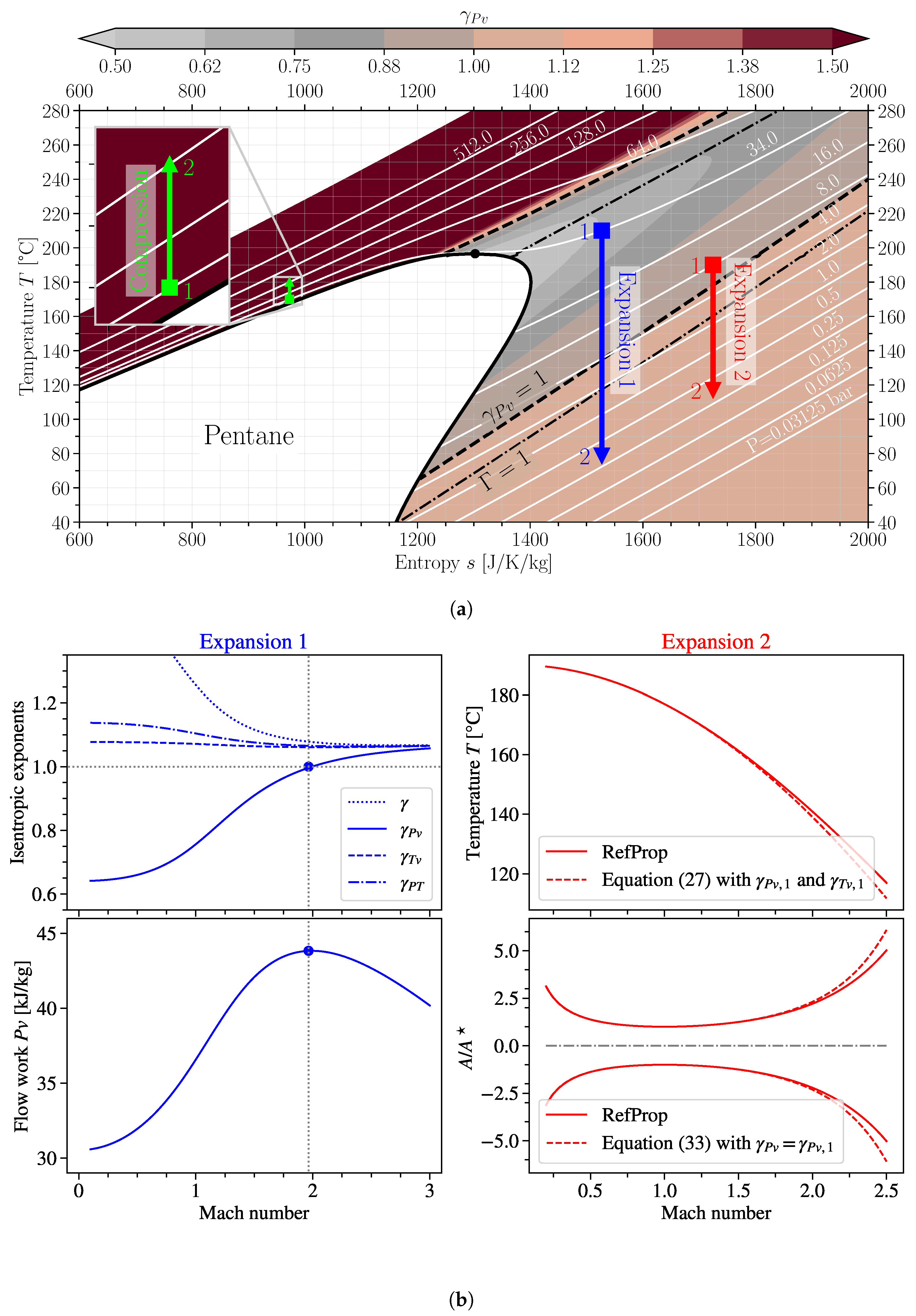
Table 1.
Limits of the exponents , , and for liquids, ideal gases, and real gases in the general case. The isentropic exponents are demonstrated to reduce to the incompressible fluid model for liquids and the ratio of the specific heats for ideal gases.
Table 1.
Limits of the exponents , , and for liquids, ideal gases, and real gases in the general case. The isentropic exponents are demonstrated to reduce to the incompressible fluid model for liquids and the ratio of the specific heats for ideal gases.
| Liquids | Real Gases | Ideal Gases | |||
|---|---|---|---|---|---|
| Limits of derivatives and isentropic exponents | |||||
Table 2.
Exemplary compression in the compressed liquid region of pentane. Bold values refer to input reference state.
Table 2.
Exemplary compression in the compressed liquid region of pentane. Bold values refer to input reference state.
| (a) Thermodynamic states | |||
|---|---|---|---|
| RefProp | Isentropic transformations Equation (2) with and (rel. error) | ||
| State | 1 | 2 | 2 |
| P [bar] | 34 | 128 | |
| T [K] | 443.15 | 453.27 | 450.60 (0.6%) |
| [kg/m] | 433.76 | 480.36 | 472.89 (1.56%) |
| 1.47 | 1.28 | ||
| 1.012 | 1.023 | ||
| 1.193 | 1.250 | ||
| (b) Enthalpy change | |||
| RefProp | (rel. error) | Isentropic Work Equation (41) with (rel. error) | |
| [kJ/kg] | 20.43 | 21.67 (6.1%) | 20.57 (0.69%) |
Disclaimer/Publisher’s Note: The statements, opinions and data contained in all publications are solely those of the individual author(s) and contributor(s) and not of MDPI and/or the editor(s). MDPI and/or the editor(s) disclaim responsibility for any injury to people or property resulting from any ideas, methods, instructions or products referred to in the content. |
© 2023 by the authors. Licensee MDPI, Basel, Switzerland. This article is an open access article distributed under the terms and conditions of the Creative Commons Attribution (CC BY) license (https://creativecommons.org/licenses/by/4.0/).
Share and Cite
MDPI and ACS Style
Nederstigt, P.; Pecnik, R. Generalised Isentropic Relations in Thermodynamics. Energies 2023, 16, 2281. https://doi.org/10.3390/en16052281
AMA Style
Nederstigt P, Pecnik R. Generalised Isentropic Relations in Thermodynamics. Energies. 2023; 16(5):2281. https://doi.org/10.3390/en16052281
Chicago/Turabian StyleNederstigt, Pim, and Rene Pecnik. 2023. "Generalised Isentropic Relations in Thermodynamics" Energies 16, no. 5: 2281. https://doi.org/10.3390/en16052281
Note that from the first issue of 2016, this journal uses article numbers instead of page numbers. See further details here.