Enhanced Control Designs to Abate Frequency Oscillations in Compensated Power System

Abstract

The interconnection of transmission, distribution, and generation lines has established a structure for the power system that is intricate. Uncertainties in the active power flow are caused by changes in load and a growing dependence on renewable energy sources. The study presented in this paper employs several controlling strategies to reduce frequency variations in series-compensated two-area power systems. Future power systems will require the incorporation of flexible AC transmission system (FACTS) devices, since the necessity for compensation in the power system is unavoidable. Therefore, a static synchronous series compensator (SSSC) is installed in both areas of our study to make it realistic and futuristic. This makes it easier to comprehend how series compensation works in a load–frequency model. With the integration of electrical vehicles (EVs) and solar photovoltaic (PV) systems, several control strategies are presented to reduce the frequency oscillations in this power system. Particle swarm optimization (PSO) is used to obtain the best PI control. To improve results, this work also covers the design of fuzzy logic control. In addition, the adoption of neural network control architecture is proposed for even better outcomes. The outcomes clearly show how well the proposed control techniques succeeded.

1. Introduction

A power system is made up of many generating units that are linked together via tie lines to meet the load demand. Due to random changes in active and reactive power demand, the system frequency and tie-line power exchange vary. To maintain the stability and reliability of the power system, the change in frequency and tie-line power exchange need to be balanced quickly. Load Frequency Control (LFC) is the process of maintaining frequency and tie-line power in a state of balance. A power system is constantly subjected to some kind of disturbance, which causes power system components to trip. When subjected to disturbance, the power system is expected to settle down to some equilibrium. If the system’s equilibrium is disturbed, the machine rotor will accelerate or decelerate in accordance with the laws of motion for rotating bodies [1].

In order to reduce frequency and voltage oscillations caused by load variations or abrupt changes in load requirements, automatic generation control (AGC) is crucial for the operation of electric power systems. Due to the increasing exploitation of renewable resources in the power system, the uncertainty in real power production has increased significantly. Additionally, load disturbances also disrupt the normal operation of a power system. The energy system has evolved into a complex unit as a result of a web of interconnected power systems and advances in electrical technology. Variations in frequency can occur in an interconnected power system due to changes in constant load demand, system characteristic uncertainty, or changes in environmental conditions. So, the stability of the power system must be maintained in the event of a temporary disruption such as overload, faults, or line tripping [2,3]. Load frequency is crucial in balancing power between load and generation. The nominal system frequency changes according to the difference between generated and load power. When the quantity of power generated becomes insufficient to meet the amount of demand, the speed or frequency of the generating units will be reduced and vice versa. So, the system must maintain an acceptable frequency [4,5]. Variations in frequency of ±3% between lightly loaded and fully loaded conditions are acceptable. A changing system frequency that exceeds a certain threshold is a potentially dangerous indicator of a real power imbalance. As a result, the power system must be robust to minimize frequency oscillations [6,7]. If a system parameter in an interconnected power system with several control areas changes, the grid-connected power will vary, and frequency deviations will happen. To ensure reliable and stable operation, the system must be kept at a predefined frequency, or the variation in load demand and supply must be adjusted in less time. Unpredictable fluctuations in load demand result in significant load and electricity generation opportunities. The generator speed changes due to this circumstance have an immediate impact on the system’s frequency. To reduce the frequency error to zero, the control system must take action. In conjunction with the system frequency, the load frequency control maintains a predetermined power flow in a contact line. To maintain the same frequency, the turbines were used to tune a proportional–integral controller that controlled the generators, and by adjusting the control parameters, the system’s steady-state frequency error was reduced [8,9]. Traditional controllers based on proportional–integral controllers have been the focus of many researchers. PI controllers do not produce adequate results when there are nonlinear components present [10,11,12]. Various methods have been proposed to tune the PI controller. Many authors have suggested using optimization algorithms, fuzzy logic, Genetic Algorithms, particle swarm optimization, and neural networks as intelligent techniques to surmount these limitations and efficiently handle the load frequency control problem [13,14,15]. Because power systems are complex, some control solutions based on traditional control techniques may not be appropriate in all operating scenarios [16,17]. If the gain in the PI controller is very high, it will result in unwanted and unacceptable overshoots [18,19]. The advantages of an electric vehicle (EV) in terms of lowering carbon emissions are significant. Nowadays, EVs are linked to the power grid, allowing for the most efficient transfer of electricity between users and the grid [20]. Mrinal Ranjan and Ravi Shankar [21] discussed increasing the load demand, the rapid depletion of fossil fuels, and newly implemented electrical deregulation policies. In addition, the Flexible AC Transmission System (FACTS) will examine possible solutions and future aspects. Debbarma and Dutta [22] address EVs in LFC in a deregulated setting. The load on the grid is balanced by a battery charger. A situation where an electrically powered car abruptly loses power and behaves in an unpleasant manner could occur. To prevent this, a frequency band limit is selected. Liu et al. [23] proposed frequency regulation using the useful car to grid control. Additionally offered are two control systems using high-frequency signals obtained from Area Control Error (ACE) and area regulation requirements. These make sense for additional research on the hybrid power system’s LFC incorporating Sustainable Transportation Systems (STS) and EVs. The power system is becoming more difficult as EV penetration grows, necessitating the requirement of an effective and dependable control-engineered layer. The majority of power systems have adopted a sophisticated centralized control system, in which fluctuations in power system load finally result in significant disruption [24]. Samy et al. [25] proposed a techno-economic feasibility analysis and a sizing method for grid-connected solar systems with various battery technologies. In [26], the proposed system control was based on monitoring the battery’s state of charge and supplying loads as efficiently as possible using renewable energy sources. For microgrid stability techniques, the performance of the following three controllers—PID, ANN, and fuzzy logic—is studied. Based on the simulation results, the fuzzy logic controller has higher efficiency and precision than the others (PID and ANN).

The motivation to work in this field of power systems comes from the fact that the effects of flexible AC transmission (FACT) devices, solar PV, and EVs are studied but not fully understood. The performance of the FACTS device can be optimized using different techniques, such as the genetic algorithm, particle gravitational search algorithm, and particle swarm optimization, as discussed in [27,28,29,30]. The power system will be analyzed and modeled for optimal power system control, which must incorporate the effects of the systems, as mentioned earlier, for the control to be effective in the future. The main contribution of this manuscript is novel fuzzy logic and neural control designs that are proposed to alleviate frequency oscillations in the interconnected power system consisting of SSSC, solar PV, and EVs. The main objective of analyzing the effects of futuristic system design on power systems has been achieved through the comparative analysis of the system model. Not only does the proposed control help us understand the system dynamics better, but it also has great efficacy in abating the oscillations.

The paper is organized with a discussion of the transfer function system model in Section 2. This is followed by the control design proposed in Section 3. Particle swarm optimization, fuzzy logic control, and neural network control design have also been discussed in the same section. In Section 4, time-domain simulations were used to demonstrate the outcomes obtained with the proposed controllers. Section 5 contains a list of the study’s conclusions, which are followed by the references.

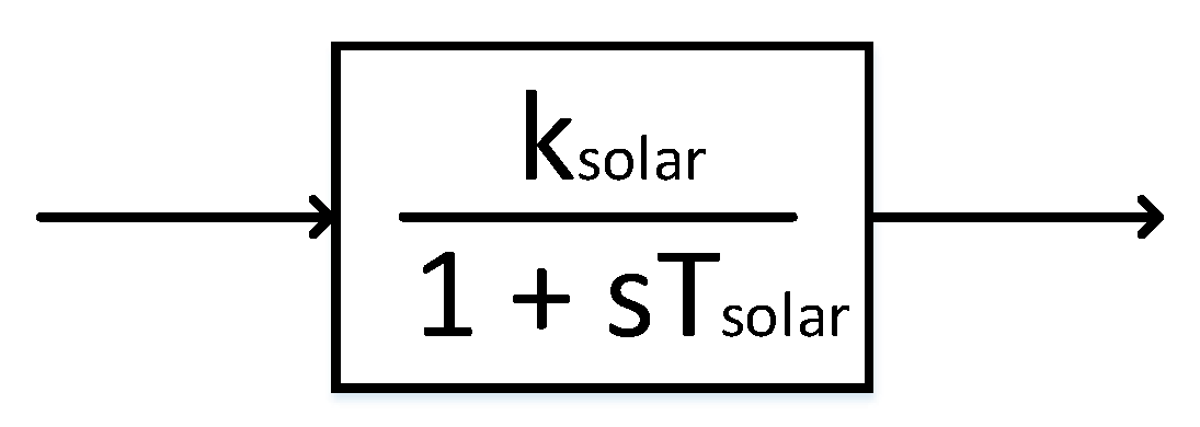
2. System Modeling

A multi-area power system is formed by connecting multiple single-area systems. Interconnection improves the stability and dependability of the power system. The system, however, becomes more complex as a result of interconnections. Each area’s frequency and voltage must be controlled and kept within set limits to protect against damage to the entire system. Based on its coherency, a large power system can be divided into several control areas. In a coherent system, generators accelerate and decelerate together while maintaining their relative power angles [31,32,33,34].

A two-area power system with hydro and thermal units is considered. Area 1 is a hydro-power plant, and Area 2 is a thermal power plant of the reheat type [35]. Thus, this work proposes a control design for a system. The controller’s goal is to reduce system frequency oscillations in both areas when a step load disturbance is applied. Control design will be discussed in the next section. A complete block diagram of the analyzed system is shown in Figure 1.

A solar PV system is made up of many PV panels, each of which has many solar cells. The basic building block of solar power generation is the solar cell. An electronic component called a photovoltaic cell produces electricity when exposed to sunlight. The solar cell can be used separately or alongside other solar cells in a photovoltaic panel. PV cell models come in a variety of forms, each with varying degrees of complexity and accuracy. The equivalent electrical circuit shown in Figure 2 can be used to model photovoltaic cells. The transfer function model for the solar system is shown in Figure 3.

The PV cell’s current is modeled by the following equation:

$$I_{Dspv}=I_{Lspv}-I_0(ex{p}^{(V_{spv}+R_{Sspv}{I}_{spv})/V_T}-1)-(V_{spv}+R_{Sspv})/R_{SHspv}$$

(1)

$$V_T=\left(N_{s}nKT\right)/q$$

(2)

where

$I_{Dspv}$: the photo-current;

$R_{SHspv},R_{Sspv}$ represents shunt and series resistance;

$I_{Lspv}$ represents the light generated curent in the cell;

$I_{SHspv}$ represents current lost due to shunt resistance;

$I_{spv},V_{spv}$ represents output current and output voltage;

$I_0$: reverse saturation currents of the diode;

$V_T$: the thermal voltage;

$N_s$: cells connected in series;

n: the diode ideality constant;

q: charge of the electron;

k: the Boltzmann constant;

T: the temperature of the p–n junction.

Because of their massive energy reserves, a large number of aggregated EVs can assist the power system’s LFC. Load frequency control, battery chargers, and primary frequency control are included in the cumulative model of EV fleets shown in Figure 4. The power exchange between the grid and the battery (Li-ion) is regulated by the battery charger. Each EV has a deadband (DB) function with droop features to prevent unwanted frequency fluctuations in the event that EVs become disconnected from the grid [36]. The values chosen for the DB’s upper limit (FUL) and lower limit (FLL) are 10 mHz. The aggregate model droop coefficient (RAG) value is assumed to be the same as for conventional plants. The EV gain and the battery time constant, respectively, are denoted by $K_{EV}$ and $T_{EV}$. The $K_{EV}$ value depends on the EVs’ state of charge (SOC) [37].

The nominal values of the two area power system model parameters are given in

Table 1. System parameters.

	Parameters	Values
Area 1	K${}_g$, $K_t$, $K_{ps},T$ $T_g,T_t,T_{ps}$, ${\beta }_1,R_1$	1, 1, 120, 0.0866 0.08 s, 0.3 s, 20 s, 0.425, −2.4
Area 2	$K_{g2},K_{t2},K_{ps2}$ $T_{g2},T_{t2},T_{ps2},T_{sh1},T_{sh2}$ ${\beta }_2,R_2$	1, 1, 120 0.08 s, 0.3 s, 20 s, 5 s, 10 s 0.425, −2.4
SSSC	$K_{SSSC}$ $T_{SSSC}$	0.2035 0.03 s
Electrical Vehicle	$R_{AG},K_{EVI}$ $T_{EVI}$ $N_{EV}$	0.24, 1 1 s 1000
Solar	$K_{solar}$ $T_{solar}$	1.8 1.8 s

:

Where $K_g$, $K_t$, $K_{ps}$, $K_{g2}$, $K_{t2}$, and $K_{ps2}$ represent the forward gain of the governor, turbine, and generator load model of area 1 and area 2, respectively. $k_{SSSC}$, $K_{solar}$, and $K_{EVI}$ represent the forward gain of SSSC, solar and an electrical vehicle.

$T_g$, $T_t$, $T_{ps}$, $T_{g2}$, $T_{t2}$, and $T_{ps2}$ represent the time constant of the governor, turbine, and generator load model of area 1 and area 2, respectively. $T_{sh1}$, $T_{sh2}$, $T_{SSSC}$, $T_{EVI}$, and $T_{solar}$ are the time constant of the reheat, SSSC, electrical vehicle and solar.

${\beta }_1$, $R_1$, ${\beta }_2$, and $R_2$ represent the bias coefficient and droop coefficient for area 1 and area 2, respectively.

$N_{EVI}$ is the number of electrical vehicles.

3. Control Design

3.1. Particle Swarm Optimization

In 1995, Particle Swarm Optimization was designed by Kennedy and Eberhard. PSO is an optimization technique to solve a problem based on the social interaction of birds. Simple software agents, known as particles, travel in the search space of an optimization problem. A particle position offers a potential solution to the optimization problem. Every particle is treated as a point in N-dimensional space. It continues to accelerate in the search space based on its knowledge about the appreciable solution, comparing its greatest value to the best value of the swarm thus far [38,39]. Three-dimensional vectors define each particle:

• Position (x): It determines the location of the ith member in the tth run of the algorithm.
• Velocity (v): It gives the direction and length of the ith member in the tth run of the algorithm.
• Personal best ($xbest$): is the ith particle’s best location up to this point.

Global best ($gbest$) is the best location in the swarm and the optimal answer to the problem. It cannot consistently give the optimal solution for the question, but the value produced is the best value and solution for the situation.The following two equations update the particle’s position and velocity.

$$v_i^{k+1}=\omega v_i^k+r_1·ran{d}_1·(xbes{t}_i-x_i^k)+r_2·ran{d}_2·(gbes{t}_i-x_i^k)$$

(3)

where k is the iteration number, $\omega$ is the inertia weight factor, $r_1$ and $r_2$ are the acceleration constants and $rand\left(\right)$ is the random value whose value lies between 0 and 1.

$$\omega ={\omega }_{max}-\frac{({\omega }_{max}-{\omega }_{min})}{k_{max}}k$$

(4)

where $k_{max}$ is the maximum number of iterations.

The equation comprises three parts. The first part is related to the urge to move or progress. The second part is related to the particle’s own memory to learn from past experience, and the third part is related to the influence of other individuals. The position is updated as

$$x_i^{k+1}=x_i^k+v_i^{k+1}$$

(5)

$x_i^{k+1}$ and $x_i^k$ represents the modified and current positions.

$v_i^{k+1}$ is modified velocity.

This process will not halt until thebest possible solution is not obtained or the number of iterations is over [40,41]. The flowchart of the algorithm is shown in Figure 5. The PSO method will produce personal and global best after each iteration, and after each iteration, PSO will give the global best value, which is the best possible solution to the problem.

3.2. Fuzzy Logic Controller

Fuzzy logic is based on fuzzy sets, where each value of a given set is tracked to any value between 0 and 1. It represents the degree of membership. The key benefit of utilizing this controller is that control parameters can be modified quickly based on system dynamics because no parameters are required when building controllers for nonlinear systems. A PI controller tuned with fuzzy logic is proposed in this study. The inputs to the fuzzy logic controller are errors and their derivatives [42,43,44,45,46]. The rule base of the designed fuzzy control is provided in

Table 2. Rule base for fuzzy controller.

A,B	VS	S	Z	B	VB
VS	S	S	M	M	VB
S	S	M	M	VB	VB
Z	M	M	VB	VB	VVB
B	M	VB	VB	VVB	VVB
VB	VB	VB	VVB	VVB	S

, with five membership functions per rule. Triangular membership functions (trimf) are implemented for both inputs and outputs. The five distinguished membership functions chosen for input are small (S), very small (VS), zero (Z), very big (VB), and big (B), and the linguistic variables chosen for output are medium (M), small (S), big (B), very very big (VVB), and very big (VB). These variables are shown in Figure 6, Figure 7, Figure 8 and Figure 9.

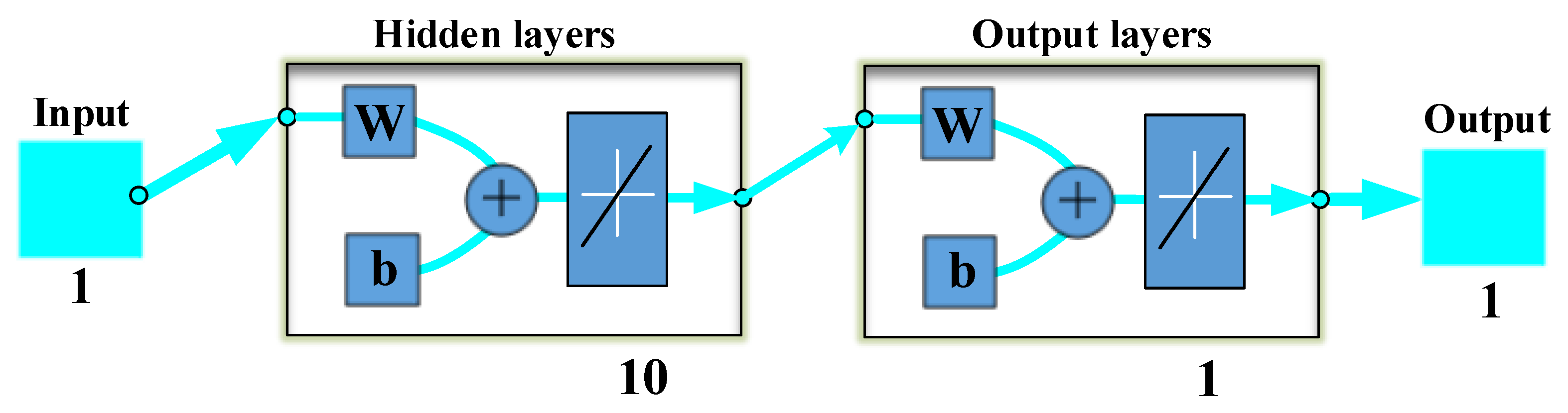
3.3. Neural Network

Warren McCulloch, a neurophysiologist, and Walter Pitts, a mathematician, proposed a threshold reasoning mathematical model of brain neurons in 1943 and showed how it may be used to compute logic functions. They used an electrical circuit to represent a simple neural network. A neural network is a powerful technique to solve real-world complications. The idea began with how neurons in the brain function. A neural network is formed by connecting one neuron to every other neuron through layers. In order to improve their performance, neural networks can learn from past experiences. In simpler terms, a neural network tries to recognize relationships, patterns, and information from the data based on a set of algorithms that simulate the human brain [47]. Complex data-driven problems can be solved using the neural approach, which mimics the behavior of the human brain to solve problems. The simplest form of a neural network consists of an input, a hidden layer, and an output layer connected via nodes as shown in Figure 10, which together form a network called a neural network.

• Input layer: These input layers/nodes receive information from the outside world and pass it to a hidden layer.
• Hidden layers: These sets of neurons perform all the computation on input data. Each hidden layer is specialized to produce a particular output for purposeful results.
• Output layers: There can be single or multiple nodes in an output layer. These receive hidden layers and perform the calculation via its neurons, and then, the output is computed.

Figure 10. Basic structure of neural network.

Figure 10. Basic structure of neural network.

The designed neural network controller has one input and one output with a 10-layer feed-forward network. The controller has been trained off-line using the Bayesian regularization algorithm. It depends on the application and what kind of architecture a neural network has as well as how many neurons are present [12,14].

The architectural diagram is shown in Figure 11. The network is calibrated in such a way that when the inputs are the same, the response will be the same. If the system unknowns can be demonstrated as not being controlled by the system parameters, then the neural network controller can be used effectively. The inputs $p_1$, $p_2$, $p_3$, …, $p_n$, and the weights $W_{1,a1}$, $W_{1,a2}$, …, $W_{1,ar}$ of the weight matrix w and the bias “b” are linked for the neuron and added with the weighted inputs [46].

A multi-input neuron is shown as,

$$n=W_{1,a1}{p}_1+W_{1,a2}{p}_2+\dots +W_{1,ar}{p}_{ar}+b$$

(6)

In matrix form,

$$N=W_{ap}+b$$

(7)

4. Results

A two-area power system, with area 1 being hydro and area 2 being thermal with reheat, is considered. This power system is incorporated with a FACTS device so that the power system under study is realistic and futuristic. A comparative analysis of the results obtained from the controllers discussed in Section 3 is provided in this section.

The effect of the FACTS device is studied on the power system, and compression between the power system that is compensated with SSSC and the uncompensated system is shown in Figure 12 and Figure 13. Results show that SSSC mitigates the frequency oscillations in both areas. A steady-state error will be present as no integral control is provided.

The result also shows comparative analysis with conventional PI, PI tuned with fuzzy logic, PSO-tuned PI, and neural networks, as shown in Figure 12 and Figure 13. Compared to other techniques, the results obtained using a neural network have minimal overshoot, and the system response is fast. The neural network method finds the best parameters for the controller. The results are analyzed based on the settling time and maximum overshoot, as given in

Table 3. Comparison Table.

Controller	Settling Time (s)		Maximum Overshoot/ Undershoot (Hz)		SSD
	Area 1	Area 2	Area 1	Area 2	Area 1	Area 2
Uncompensated	31	25	0.022	0.022	0.013	0.013
Proportional-Integal	28	28	0.0008	0.001	0	0
PSO	19	15	0.00065	0.0025	0	0
Neural Network	8	7	0.0005	0.0012	0	0
FLC	18	14	0.0012	0.005	0	0

.

4.1. Case 1: Two-Area Power System with Solar Alone

The effect of the incorporation of solar on the system is shown in Figure 14 and Figure 15. There is an increase in the frequency deviations and settling time of the power system as compared to the two-area power system.

4.2. Case 2: Two-Area Power System with EV Alone

Figure 16 and Figure 17 show EV alone is incorporated in the two-area power system, resulting in higher frequency oscillations and setting time for the system when compared to the two-area power system.

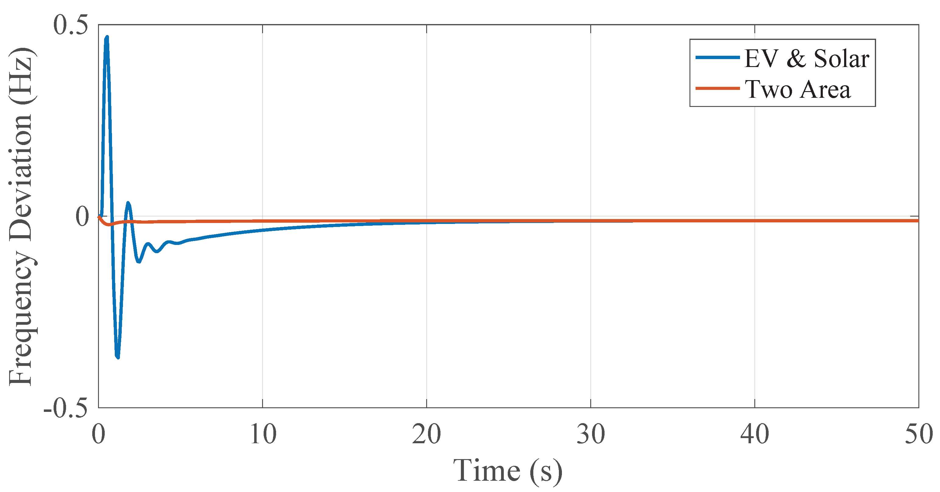
4.3. Case 3: Two-Area Power System with Solar and EV

4.3.1. SSSC Based System

In Figure 18 and Figure 19, the effect of SSSC is studied on a system with two-area power systems and a system with EV and solar. The frequency deviations in a power system with EV and solar incorporated are greater than in a two-area power system. These oscillations have a higher amplitude and persist for a longer duration, which is evident from the settling time when the two systems are compared. The results also show that SSSC successfully mitigates the frequency oscillations in both systems.

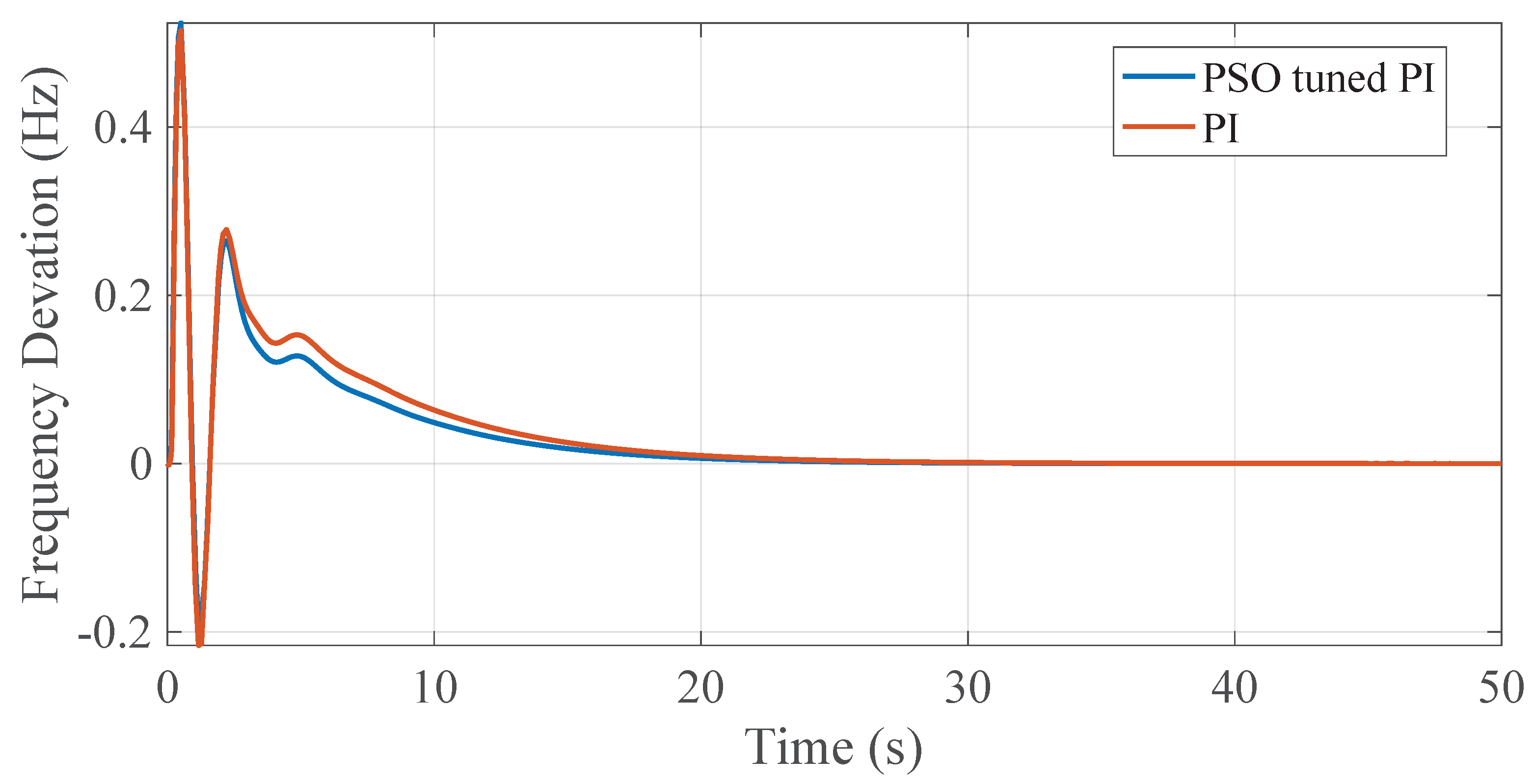
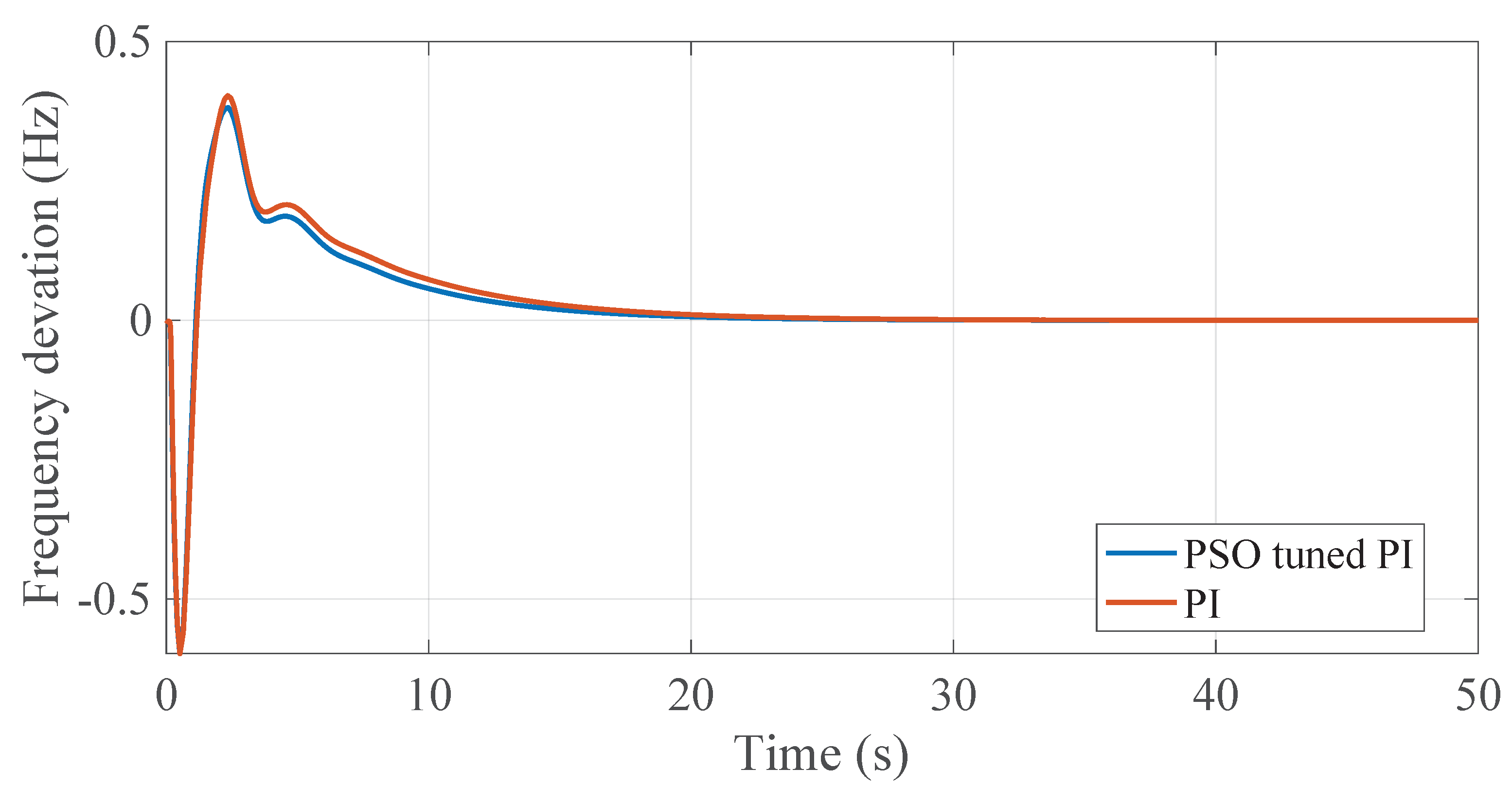
4.3.2. PSO-Tuned PI and Conventional PI

The comparative analysis of the PSO-tuned PI and conventional PI controllers is given in Figure 20 and Figure 21. The PI has been tuned by the Ziegler–Nichols method and by PSO. The values of $K_p$, $K_i$, and $K_d$ obtained in PSO-tuned PI for the system are slightly better in terms of settling time.

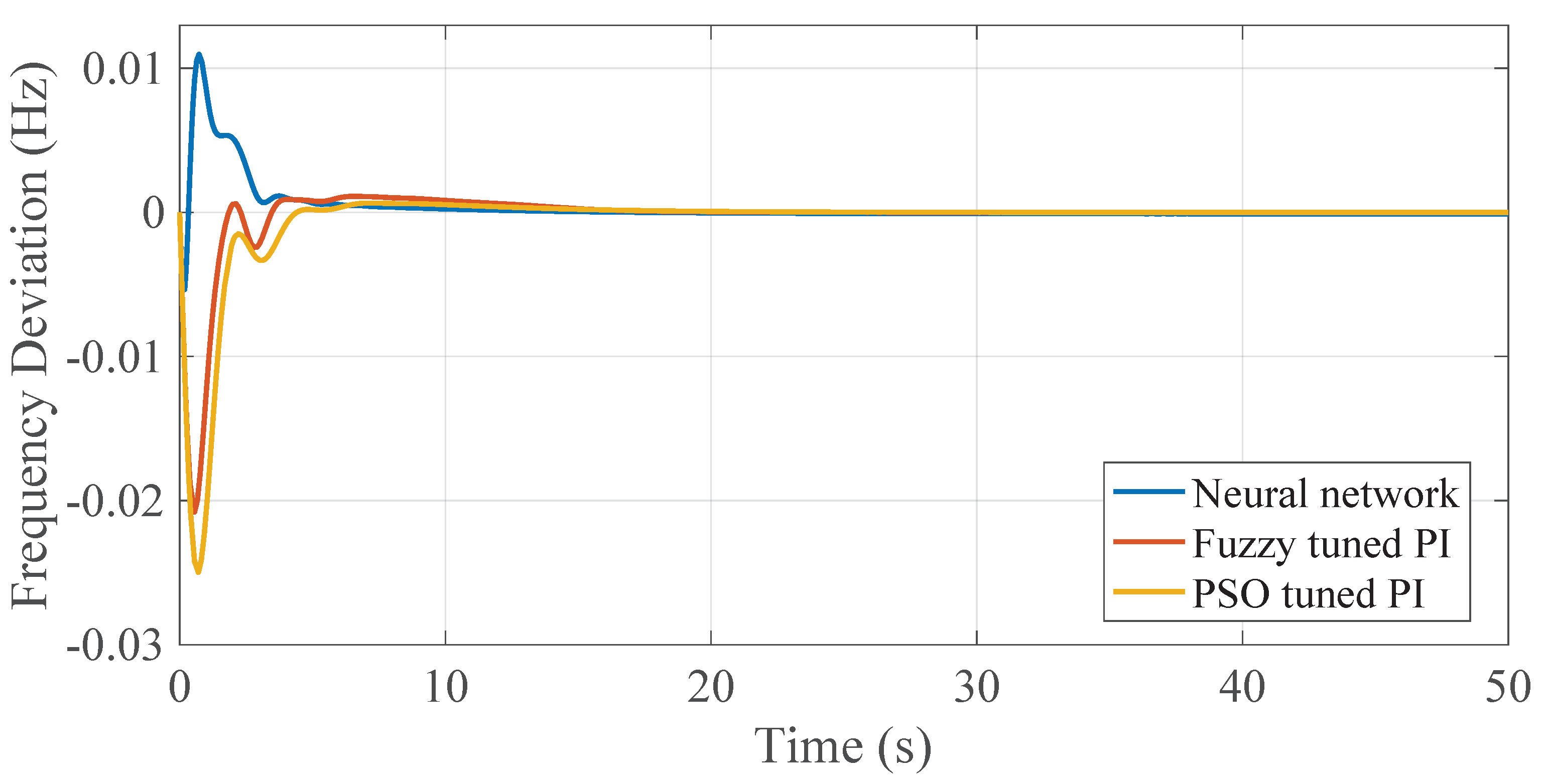
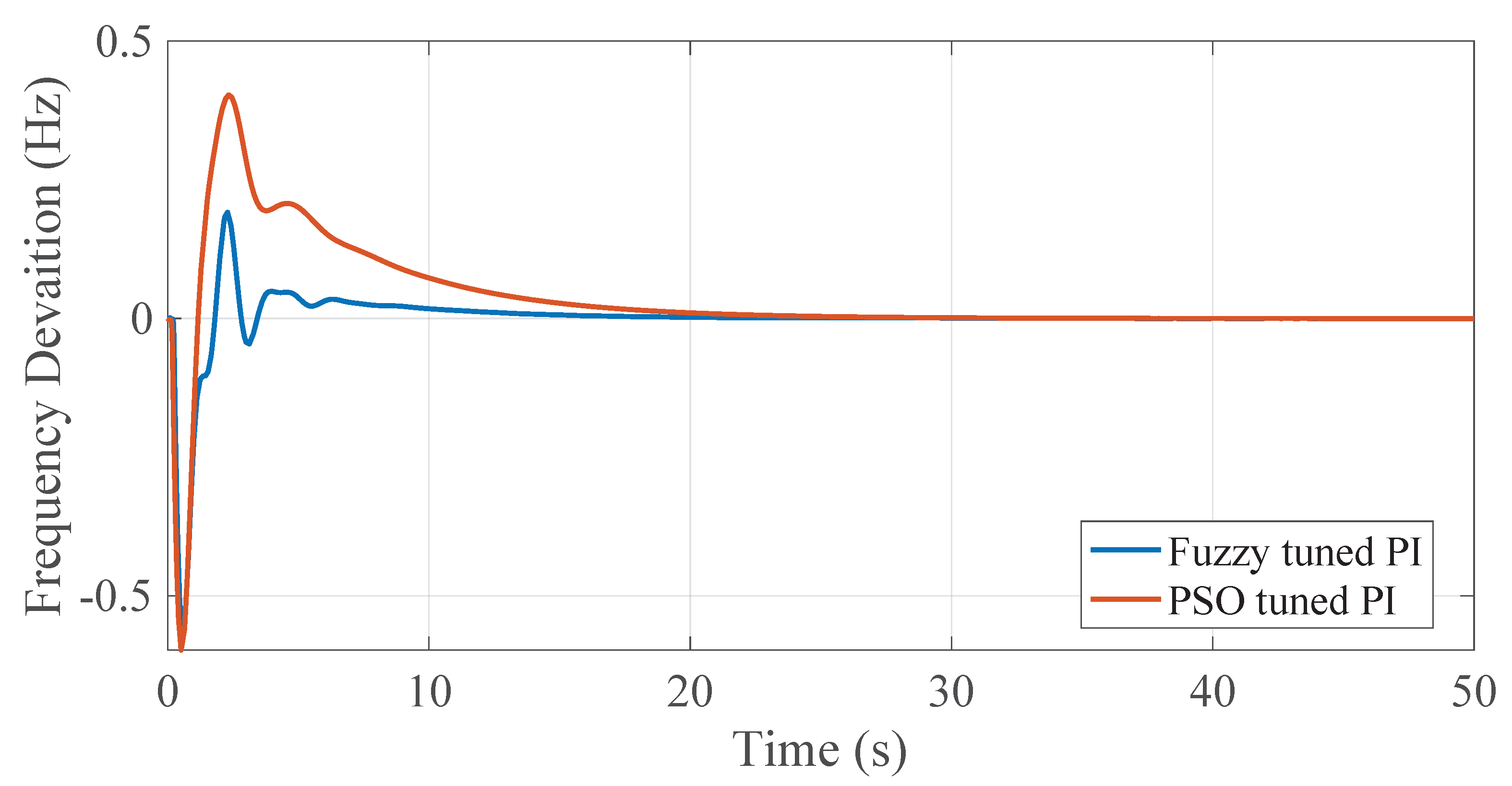
4.3.3. Comparative Analysis of Fuzzy-Tuned PI and PSO-Tuned PI

Figure 22 and Figure 23 shows the comparative analysis of a fuzzy-tuned PI and a PSO-tuned PI, respectively. A fuzzy logic controller provides more optimal values for the system controller. The settling time in the fuzzy logic controller for area 1 and area 2 is about 18 and 16 s, respectively; for PSO, it is about 23 and 22 s. The oscillations in the system are more using fuzzy in area 1 than in PSO, but these oscillations mitigate at a very fast rate. In area 2, the peak overshoot and undershoot for fuzzy are much better, and the system also settles fast.

4.3.4. Fuzzy-Tuned PI and Neural Network

A neural network makes the system’s response better and faster as compared to fuzzy-tuned PI. The settling time of the system is significantly reduced to 8 s and 7 s for area 1 and area 2, respectively. Oscillations in the system have been significantly reduced, as can be shown in Figure 24 and Figure 25.

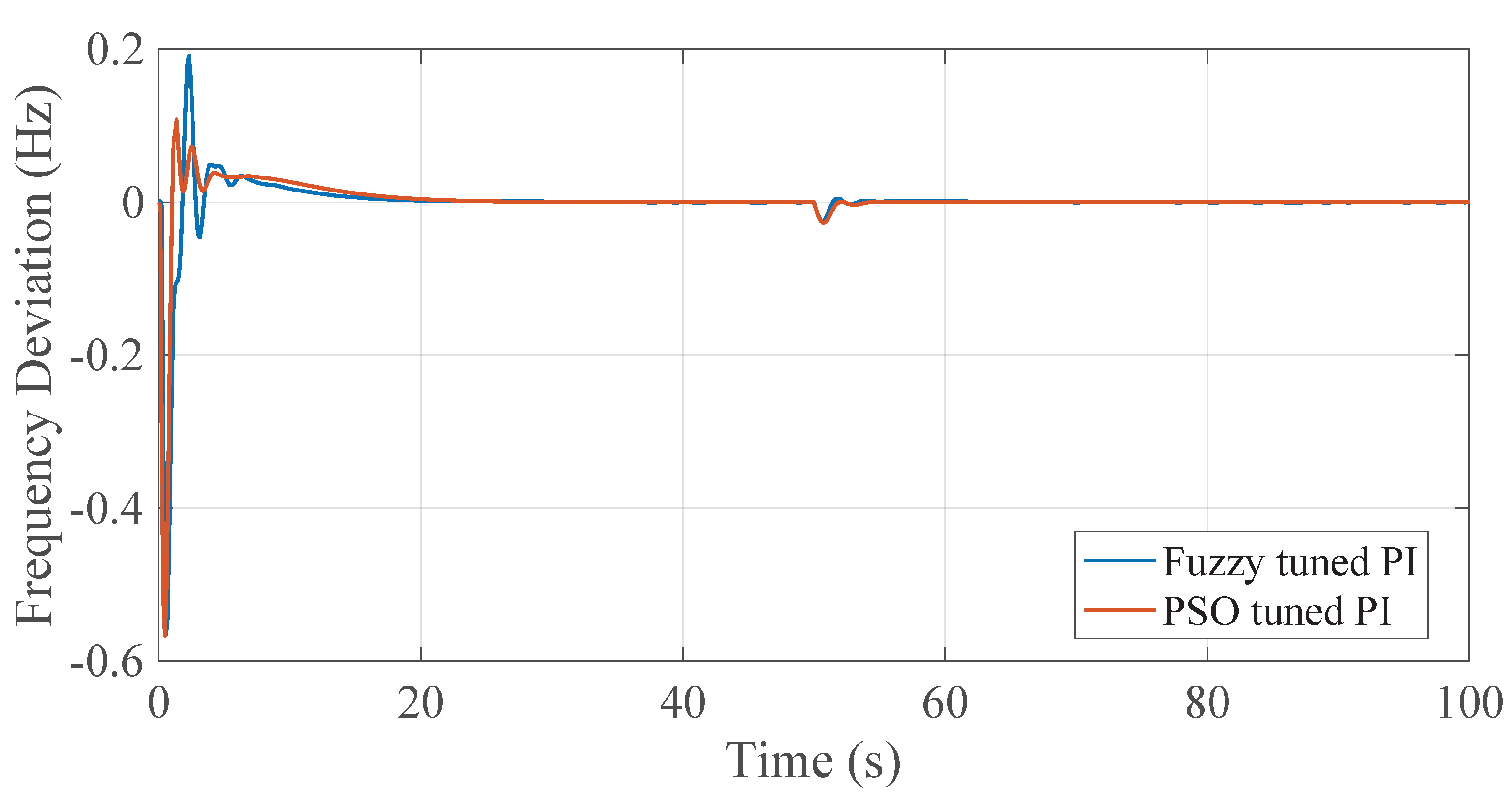
4.4. Comparison between Neural Network, Fuzzy-Tuned PI and PSO-Tuned PI

Figure 26 and Figure 27 give the comparative analysis of three control schemes, i.e., neural network, fuzzy logic controller, and partial swarm optimization. PSO makes the system slightly better than a conventional PI controller by reducing the settling times of area 1 and area 2 to 23 s and 22 s, respectively. A fuzzy logic controller further optimizes the values of the controller and reduces the system settling times to 18 and 16 s, respectively. The neural network provides the best results for the system as the settling time reduces to 8 s for area 1 and 7 s for area 2. The frequency of oscillations in the system using a neural network is reduced as compared to the other two controllers. The comparison in

Table 4. Comparison table of two-area power systems with solar and EV incorporated.

Controller	Settling Time (s)		Maximum Overshoot/Undershoot (Hz)
	Area 1	Area 2	Area 1	Area 2
PSO	23	22	0.5	0.6
FLC	18	16	0.58	0.6
Neural Network	8	7	0.58	0.58

shows these controllers’ settling time and maximum overshoot and undershoot.

4.5. Disturbance

In Figure 28 and Figure 29, another disturbance of magnitude 0.05 PU is given to the system after 50 s. As seen from the figures, it is evident the controller is robust enough to compensate for any disturbance, as the system settles in less than 5 s in both areas and there are minimum oscillations.

5. Conclusions

The purpose of this work is to propose a two-area SSSC-based model of the power system with solar and EV integration in order to have a futuristic and realistic study on load frequency control. In order to reduce frequency oscillations, the research demonstrates implementing fuzzy logic and neural network control designs. The PSO-tuned PI controller has been compared with both control strategies for reducing frequency oscillations. The findings of this manuscript demonstrate the effectiveness of the proposed control schemes. To highlight the main conclusions, first, a compensated system operating without a controller reduces frequency oscillations but is unable to attain zero steady-state error. Additionally, SSSC can reduce frequency oscillations, but it is unable to stabilize the system on its own. Indeed, the effects of solar PV and electric vehicles (EVs) on the system’s frequency are distinct and dynamic. Additionally, a tuned PI controller enhances the system’s responsiveness and achieves 0% steady-state error. The PSO offers PI tuning that is ideal with a slightly swift response. In the end, the fuzzy-tuned PI controller produces better outcomes than the PSO with a fast response. As a result, when compared to other controllers, the results demonstrate that neural networks produce better results, as seen by their quick settling time and smaller maximum overshoot.

References

- Kothari, D.P.; Nagrath, I.J. Modern Power System Analysis; McGraw Hill: New York, NY, USA, 2003. [Google Scholar]
- Kundur, P. Power System Stability and Control; McGraw Hill: New York, NY, USA, 1994. [Google Scholar]
- Bevrani, H. Robust Power System Control; Springer International Pulbishing: Cham, Switzerland, 2014. [Google Scholar]
- Umrao, R.; Kumar, S.; Mohan, M.; Chaturvedi, D.K. Load Frequency Control methodologies for power system. In Proceedings of the 2nd International Conference on Power, Control and Embedded Systems, Allahabad, India, 17–19 December 2012; pp. 1–10. [Google Scholar]
- Guven, A.F.; Samy, M.M. Performance Analysis of Autonomous Green Energy System Based on Multi and Hybrid Metaheuristic Optimization Approaches. Energy Convers. Manag. J. 2022, 269, 116058. [Google Scholar] [CrossRef]
- Saadat, H. Power System Analysis; McGraw Hill: New York, NY, USA, 2002. [Google Scholar]
- Rajan, R.; Fernandez, F.M. Impact of Increased Penetration of Photovoltaic Sources on Small-Signal Stability of Hybrid and Multi-area Power Systems. In Proceedings of the 2019 Innovations in Power and Advanced Computing Technologies (i-PACT), Vellore, India, 22–23 March 2019; pp. 1–6. [Google Scholar]
- Barakat, S.; Emam, A.; Samy, M.M. Investigating grid-connected green power systems’ energy storage solutions in the event of frequent blackouts. Energy Rep. 2022, 10, 5177–5191. [Google Scholar] [CrossRef]
- Arora, K.; Kumar, A.; Kamboj, V.K. Automatic Generation Control and Load Frequency Control: A Comprehensive Review; Springer: Berlin/Heidelberg, Germany, 2019; Volume 553, pp. 449–456. [Google Scholar]
- Alhelou, H.H.; Hamedani-Golshan, M.E.; Zamani, R.; Heydarian-Forushani, E.; Siano, P. Challenges and Opportunities of Load Frequency Control in Conventional, Modern and Future Smart Power Systems: A Comprehensive Review. Energies 2018, 11, 2497. [Google Scholar] [CrossRef] [Green Version]
- Kim, J.-Y.; Kim, H.-M.; Kim, S.-K.; Jeon, J.-H.; Choi, H.-K. Designing an Energy Storage System Fuzzy PID Controller for Microgrid Islanded Operation. Energies 2011, 4, 1443–1460. [Google Scholar] [CrossRef] [Green Version]
- Syan, S.; Biswal, G.R. Frequency control of an isolated hydro power plant using artificial intelligence. In Proceedings of the IEEE Workshop on Computational Intelligence: Theories, Applications and Future Directions (WCI), Kanpur, India, 14–17 December 2015; pp. 1–5. [Google Scholar]
- Al-Majidi, S.D.; Kh. AL-Nussairi, M.; Mohammed, A.J.; Dakhil, A.M.; Abbod, M.F.; Al-Raweshidy, H.S. Design of a Load Frequency Controller Based on an Optimal Neural Network. Energies 2022, 15, 6223. [Google Scholar] [CrossRef]
- Samy, M.M.; Almamlook, R.E.; Elkhouly, H.I.; Barakat, S.T. Design Decision-Making and Optimal Design of Green Energy System Based on Statistical Methods and Artificial Neural Network Approaches. Sustain. Cites Soc. J. 2022, 84, 104015. [Google Scholar] [CrossRef]
- Verma, R.; Pal, S. Intelligent Automatic Generation Control of Two-Area Hydrothermal Power System Using ANN and Fuzzy Logic. In Proceedings of the 2013 International Conference on Communication Systems and Network Technologies, Tiruchengode, India, 4–6 July 2013; pp. 552–556. [Google Scholar]
- Mokhtara, C.; Negrou, B.; Settou, N.; Settou, B.; Samy, M.M. Design Optimization of Off-grid Hybrid Renewable Energy Systems Considering the Effects of Building Energy Performance and Climate Change: Case Study of Algeria Energy. Energy 2021, 219, 119605. [Google Scholar] [CrossRef]
- FatiGüven, A.; Yörükeren, N.; Samy, M.M. Design optimization of a stand-alone green energy system of university campus based on Jaya-Harmony Search and Ant Colony Optimization algorithms approaches. Energy 2022, 253, 124089. [Google Scholar]
- Kouba, N.E.Y.; Menaa, M.; Hasni, M.; Boudour, M. Load Frequency Control in multi-area power system based on Fuzzy Logic-PID Controller. In Proceedings of the IEEE International Conference on Smart Energy Grid Engineering (SEGE), Oshawa, ON, Canada, 17–19 August 2015; pp. 1–6. [Google Scholar]
- Balamurugan, C.R. Three area power system load frequency control using fuzzy logic controller. Int. J. Appl. Power Eng. 2018, 7, 18–26. [Google Scholar] [CrossRef]
- Yang, J.; Zeng, Z.; Tang, Y.; Yan, J.; He, H.; Wu, Y. Load Frequency Control in Isolated Micro-Grids with Electrical Vehicles Based on Multivariable Generalized Predictive Theory. Energies 2015, 8, 2145–2164. [Google Scholar] [CrossRef]
- Ranjan, M.; Shanka, R. A literature survey on load frequency control considering renewable energy integration in power system: Recent trends and future prospects. J. Energy Storage 2022, 45, 103717. [Google Scholar] [CrossRef]
- Debbarma, S.; Dutta, A. Utilizing Electric Vehicles for LFC in Restructured Power Systems Using Fractional Order Controller. IEEE Trans. Smart Grid 2017, 8, 2554–2564. [Google Scholar] [CrossRef]
- Liu, H.; Huang, K.; Yang, Y.; Wei, H.; Ma, S. Real-time vehicle-to-grid control for frequency regulation with high frequency regulating signal. Prot. Control Mod. Power Syst. 2018, 3, 1–8. [Google Scholar] [CrossRef]
- Liu, F.; Song, Y.H.; Ma, J.; Mei, S.; Lu, Q. Optimal load-frequency control in restructured power systems. IET Proc. Gener. Transm. Distrib. 2003, 150, 87–95. [Google Scholar] [CrossRef]
- Samy, M.M.; Emam, A.; Tag-Eldin, E.; Barakat, S. Exploring energy storage methods for grid-connected clean power plants in case of repetitive outages. J. Energy Storage 2022, 54, 5177–5191. [Google Scholar] [CrossRef]
- Sumarmad, K.A.A.; Sulaiman, N.; Wahab, N.I.A.; Hizam, H. Energy Management and Voltage Control in Microgrids Using Artificial Neural Networks, PID, and Fuzzy Logic Controllers. Energies 2022, 15, 303. [Google Scholar] [CrossRef]
- Eslami, M.; Shareef, H.; Mohamed, A.; Khajehzadeh, M. PSS and TCSC Damping Controller Coordinated Design Using GSA. Energy Procedia 2012, 14, 763–769. [Google Scholar] [CrossRef] [Green Version]
- Eslami, M.; Shareef, H.; Mohamed, A.; Khajehzadeh, M. Damping Controller Design for Power System Oscillations Using Hybrid GA-SQP. Int. Rev. Electr. Eng. 2012, 6, 888–896. [Google Scholar]
- Eslami, M.; Shareef, H.; Mohamed, A.; Khajehzadeh, M. Optimal location of PSS using improved PSO with chaotic sequence. In Proceedings of the International Conference on Electrical, Control and Computer Engineering 2011 (InECCE), Kuantan, Malaysia, 21–22 June 2011; pp. 253–258. [Google Scholar]
- Eslami, M.; Shareef, H.; Mohamed, A. Optimization and Coordination of Damping Controls for Optimal Oscillations Damping in Multi-Machine Power System. Int. Rev. Electr. Eng. 2011, 6, 1984–1993. [Google Scholar]
- Divya, K.C.; Rao, P.S.N. A simulation model for AGC studies of hydro-hydro systems. Int. J. Electr. Power Energy Syst. 2005, 27, 335–342. [Google Scholar] [CrossRef]
- Sabahi, K.; Sharifi, A.; Aliyari Shoorehdeli, M.; Teshnehlab, M.; Aliasghary, M. Load frequency control in interconnected power system using multi-objective PID controller. In Proceedings of the 2008 IEEE Conference on Soft Computing in Industrial Applications. International Conference on Control, Muroran, Japan, 25–27 June 2008; pp. 217–221. [Google Scholar]
- Mover, W.G.P.; Supply, E. Hydraulic turbine and turbine control models for system dynamic studies. IEEE Trans. Power Syst. 1992, 7, 167–179. [Google Scholar]
- IEEE Power Energy Society. Dynamic Models for Turbine Governors in Power System Studies; Technical Report PES-TR1i; IEEE Power Energy Society: New York, NY, USA, 2013. [Google Scholar]
- Prakash, S.; Sinha, S.K. Four area Load Frequency Control of interconnected hydro-thermal power system by Intelligent PID control technique. In Proceedings of the Students Conference on Engineering and Systems, Allahabad, India, 16–18 March 2012; pp. 1–6. [Google Scholar]
- Farooq, Z.; Rahman, A.; Lone, S.A. Load frequency control of multi-source electrical power system integrated with solar-thermal and electric vehicle. Int. Trans. Electr. Energy Syst. 2021, 31, e12918. [Google Scholar] [CrossRef]
- Izadkhast, S.; Garcia-Gonzalez, P.; Frías, P. An aggregate model of plug-in electric vehicles including distribution network characteristics for primary frequency control. IEEE Trans. Power Syst. 2015, 30, 2987–2998. [Google Scholar] [CrossRef]
- Prasad, B.; Prasad, C.D.; Kumar, G.P. Effect of load parameters variations on AGC of single area thermal power system in presence of integral and PSO-PID controllers. In Proceedings of the 2015 Conference on Power, Control, Communication and Computational Technologies for Sustainable Growth (PCCCTSG), Kurnool, India, 11–12 December 2015; pp. 64–688. [Google Scholar]
- Rao, R.N.; Reddy, P.K. PSO based tuning of PID controller for a Load frequency control in two area power system. Int. J. Eng. Res. Appl. 2015, 1, 1499–1505. [Google Scholar]
- Kennedy, J.; Eberhart, R. Particle swarm optimization. In Proceedings of the ICNN’95—International Conference on Neural Networks, Perth, WA, Australia, 27 November–1 December 1995. [Google Scholar]
- Ghatuari, I.; Mishra, N.; Sahu, B.K. Performance analysis of automatic generation control of a two area interconnected thermal system with nonlinear governor using PSO and DE algorithm. In Proceedings of the International Conference on Energy Efficient Technologies for Sustainability, Nagercoil, India, 10–12 April 2013; pp. 1262–1266. [Google Scholar]
- Sreenath, A.; Atre, Y.R.; Patil, D.R. Two area load frequency control with fuzzy gain scheduling of PI controller. In Proceedings of the First International Conference on Emerging Trends in Engineering and Technology, Nagpur, India, 16–18 July 2008. [Google Scholar]
- Jain, S.K.; Bhargava, A.; Pal, R.K. Three area power system load frequency control using fuzzy logic controller. In Proceedings of the 2015 International Conference on Computer, Communication and Control (IC4), Indore, India, 10–12 September 2015; pp. 1–6. [Google Scholar]
- Kamarposhti, M.A.; Shokouhandeh, H.; Alipur, M.; Colak, I.; Zare, H.; Eguchi, K. Optimal Designing of Fuzzy-PID Controller in the Load-Frequency Control Loop of Hydro-Thermal Power System Connected to Wind Farm by HVDC Lines. IEEE Access 2022, 10, 63812–63822. [Google Scholar] [CrossRef]
- Yousuf, V.; Ahmad, A. Optimal design and application of fuzzy logic equipped control in STATCOM to abate SSR oscillations. Int. J. Circuit Theory Appl. 2021, 49, 4070–4087. [Google Scholar] [CrossRef]
- Lone, A.H.; Yousuf, V.; Prakash, S.; Bazaz, M.A. Load Frequency Control of Two Area Interconnected Power System using SSSC with PID, Fuzzy and Neural Network Based Controllers. In Proceedings of the 2nd IEEE International Conference on Power Electronics, Intelligent Control and Energy Systems (ICPEICES), Delhi, India, 22–24 October 2018; pp. 108–113. [Google Scholar]
- Prakash, S.; Sinha, S.K. Application of artificial intelligence in load frequency control of interconnected power system. Int. J. Eng. Sci. Technol. 2011, 3, 264–275. [Google Scholar] [CrossRef]