Optimization of Setting Angle Distribution to Suppress Hump Characteristic in Pump Turbine

Abstract

Pump turbines play a quite important role of peak-valley shifting in the grid, and the hump margin is a critical criterion related to the safety and stability of operation in pump mode. Aiming at investigating the influence of runner outlet setting angle distribution on hump performance of a pump turbine, three runners with different linear distributions of setting angle at outlet were proposed, and the corresponding hump performance comparison was analyzed numerically through the SST k-ω turbulent model. The numerical result shows that, compared to the experiment, the relative errors of all simulated performances (energy characteristic, torque characteristic, and efficiency) were within 3%. Moreover, it was found that setting angle distribution modes could lead to a remarkably different performance in the hump region and, for the runner whose setting angle at shroud was 10° larger than that at hub, the hump safety margin could be increased from 4% to 4.5%. Thereafter, the corresponding mechanisms including energy input and hydraulic loss were investigated through the Euler head theory and the entropy method, respectively. It was found that hydraulic loss distribution played a more important role than the input energy on controlling hump performance. Moreover, for the runner with the largest hump margin, the hydraulic loss was distributed more evenly in the decreasing discharge direction, contributing to the elimination of hump performance. In addition, hydraulic loss distribution was calculated through local entropy production rate (LEPR) method. For all proposed runners, when the pump turbine entered the hump region from a normal operation point, the hydraulic loss was mainly concentrated in vaneless areas and guide/stay vane channels, while the runner with a large setting angle at shroud could better control the hydraulic loss distribution in both the spatial location and the discharge varying direction, increasing the hump margin. The design method presented in our paper is more likely to be applied in engineering applications.

1. Introduction

With the increasing demand for clean energy, renewable energy sources are gradually being integrated into the power grid. However, renewable energy such as wind and solar energy cannot continuously and stably provide electric energy, challenging the security of the power grid. Currently, the pumped storage power plant is known as the only reliable and commercial method for energy storage, ref. [1] playing an important role in peak load shifting. When a pump turbine strays into the hump region at pump mode, the accompanying pressure fluctuation seriously affects the security and stability of the pumped storage unit. Up to now, many studies related to the generation mechanism of hump region have been carried out.

Gentner et al. [2] reported that the hump margin of the pump mode should be large enough, especially at the highest head of the pump mode since the flow characteristics in large guide vane opening are more stable according to both experimental results and numerical ones. Jia et al. [3] found that with the increase of GVO, the hump region occurs in smaller discharge operating points. Ješe et al. [4] explained that the hump region is related to the circumferential motion of the rotating stall, which is strongly related to the GVO level. Moreover, computational fluid dynamics (CFD) has been widely used to capture flow details and can provide rich information on hydraulic loss in the whole fluid field. With the help of CFD, Yao et al. [5] investigated the flow characteristic in the hump region of a model pump turbine and found that the complex flow (secondary flow, backflow, and vortex) in the vaneless region contributes to the rapid increase of energy loss, leading to the development of the hump region. In the traditional energy loss analysis process, the hydraulic loss can only be calculated by evaluating the total pressure drop, while the specific level and distribution of hydraulic loss can only be evaluated by flow characteristics. Li et al. [6] proposed the local entropy production theory to quantitively describe hydraulic loss variation in the hump region and found that the hydraulic loss near the runner inlet is sensitive to the discharge variation. Qin et al. [7,8] found that the hydraulic loss is strongly related to the vortex evolution process when the investigated pump turbine is operating in pump mode.

Under some special conditions, the hump characteristics show variability, and the hump safety margin might be insufficient. For example, the hump region shown in the energy-discharge curve is different in the discharge increase direction and the discharge decrease direction [9,10]. Cavitation is another factor that affects the hump margin, Li [11] pointed out that, when the cavitation intensity increases, the corresponding Euler head will decrease simultaneously, increasing the hydraulic loss and decreasing the energy characteristic sharply compared to the no-cavitation situation. Anciger [12] found that cavitation models can provide more-reliable and efficient predictions about the hump region through comparing numerical results and experimental data for different Thoma numbers. Liu [13] found that, if we decrease the kinematic eddy viscosity in the region whose volume fraction of water vapor is high, the prediction accuracy for the hump region will be largely increased. Based on the new cavitation method, key cavitation regions (inlet of the runner suction side) that appear in the hump region can be accurately captured.

On the other hand, people try to find out methods to eliminate the hump region. Yang [14] optimized the blade geometry with the help of the inverse design method and revealed that an after-loaded runner can effectively increase the hump margin compared to the original design. Olimstad [15] found out that the hump region is very sensitive to the geometry of the high-pressure side; even a slight variation of design parameters (radius, radius of curvature, blade angle) will obviously change the energy-discharge characteristics. Zhu [16,17] found that the blade leaning direction can affect the hump region: the hump margin of a large negative blade lean is larger than that of a large positive angle. Ran [18] rearranged the setting angle distribution at the runner outlet, namely, increasing the blade setting angle at middle span and decreasing the blade setting angle at the hub and shroud. Numerical simulation results showed that the pressure at the runner outlet was more uniformly distributed after optimization. Liu [19] adopted the groove method to control the stall in the guide vanes and demonstrated that the groove method can efficiently weaken the hump characteristic caused by rotation stall. Xue [20] found that a runner with fewer blades and larger blade wrap angles can effectively suppress the segregation near the low-pressure side of the blade, contributing to the increase of the hump margin.

The investigations reveal that the vortex evolution between guide vanes and runner blades is the main cause of the hump region in the pump mode of a pump turbine. However, the elimination mechanism of the hump region has not been investigated and revealed thoroughly. The main object of our paper is to find out the influence of setting angle distribution on the hump performance in pump mode. In our study, to avoid the deficiency of the traditional design strategy, the three-dimensional flow characteristic at the runner outlet was taken into consideration. Thereafter, three runners with different distribution rules of setting angle at runner outlet were proposed. Moreover, typical operation points in the hump region were chosen to analyze the effect of setting angle on the hump characteristics with the aid of ANSYS-CFX software. Finally, analysis and comparison of the hump characteristics of different runners was carried out in detail through the Euler head theory and the hydraulic loss method.

2. Numerical Model

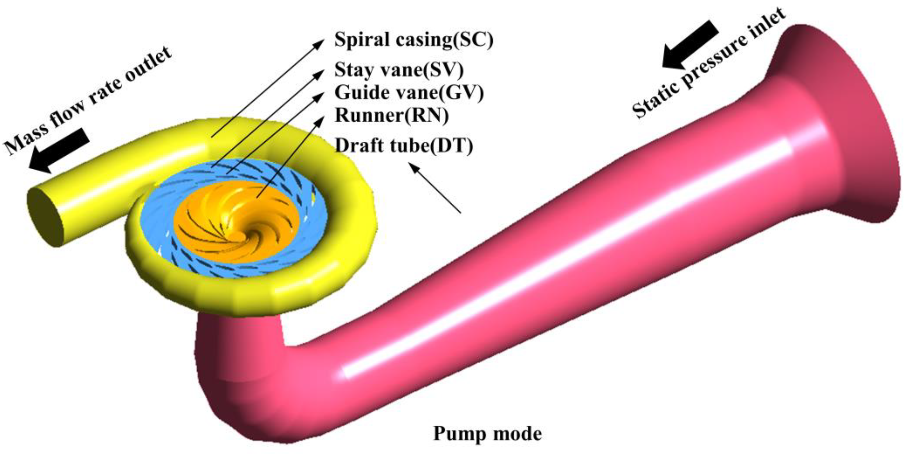
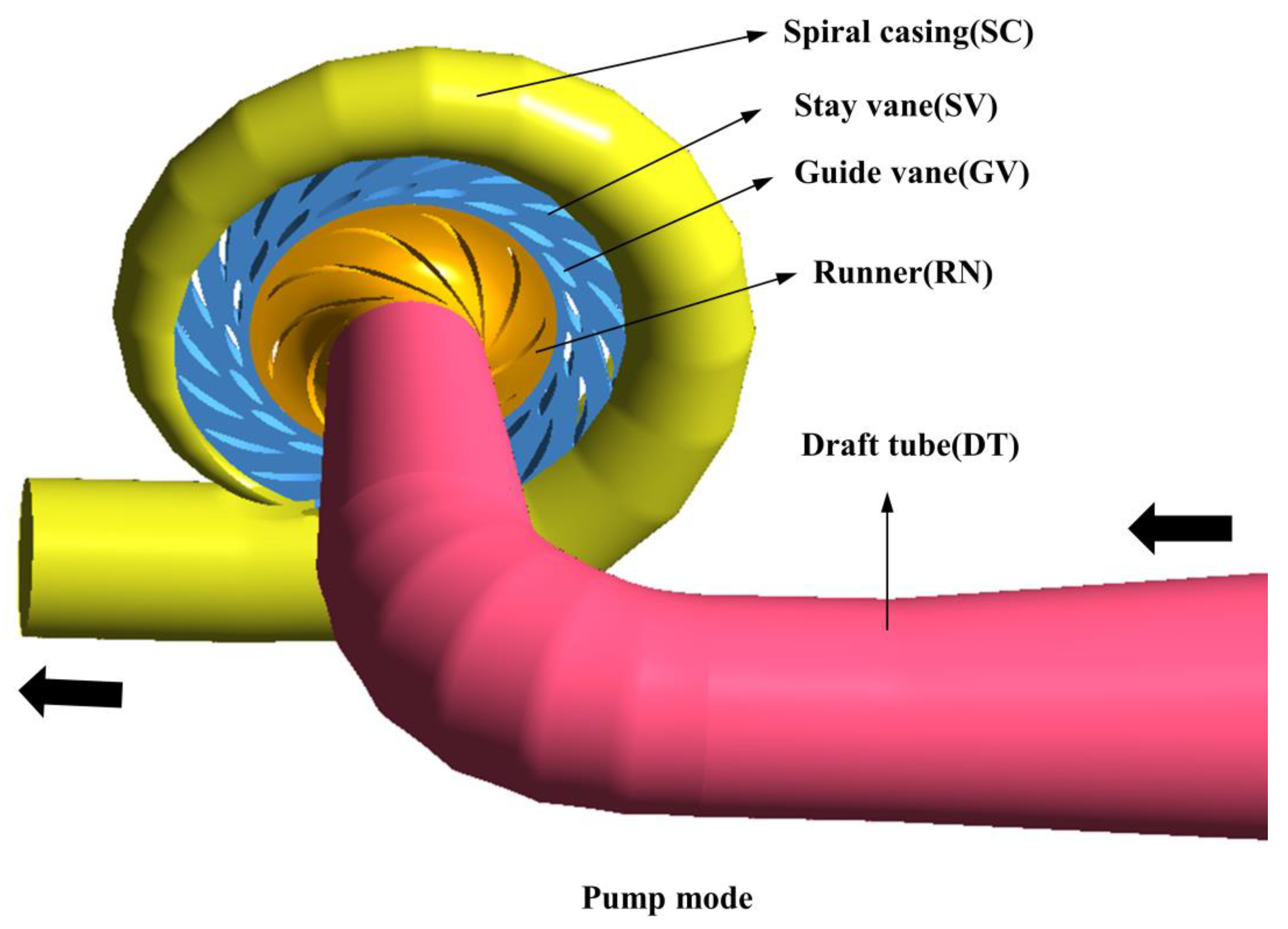
2.1. Pump Turbine Model

In our study, the fluid domain consisted of four parts, namely, the draft tube, the runner, the stay/guide vane, and the spiral casing. Figure 1 presents the established 3D computational region through UX 11.0. The head of the investigated pump turbine was 425 m, and the specific speed (n_q) was 36.1 (m, m³/s). The detailed operation and the geometric parameters of the scaled pump turbine model are presented in

Table 1. Parameters of the pump turbine.

Description	Symbol	Value
Distribution diameter of the guide vane	D0	540 mm
Runner inlet in pump mode	D1	450 mm
Runner outlet in pump mode	D2	250 mm
Runner blade number	Zr	9
Guide vane number	Zg	20
Stay vane number	Zs	20
Guide vane height	B0	43.73 mm

.

“Hump region” or “hump characteristic” in the present paper refers to the unsteady operation region in the energy-discharge curve when a pump turbine is working in pump mode, which is shown and marked in Figure 2. Moreover, the hump margin is the standard for evaluating the hump characteristic, and the hump margin is defined in (1). H_v and H_r are the head at valley point and rated point, respectively. In the present paper, the three runners in our case share the same H_r; hence, just increasing H_v can effectively increase the hump margin (eliminate the hump characteristic).

$$\mathrm{Hump} \mathrm{margin}=\frac{H_{\mathrm{v}}-H_{\mathrm{r}}}{H_{\mathrm{r}}}$$

(1)

A previous study [21] shows that a pump turbine shows different hump characteristics under different GVOs. In engineering applications, only the hump margin/hump performance at the smallest guide vanes’ opening is defined as the hump margin, and a 13 mm guide vane opening is exactly the smallest guide vane opening in our case. Hence, in the present study, the hump performance under 13 mm guide vane opening (GVO) was investigated.

2.2. Numerical Method and the Boundary Conditions

In this study, the finite volume method was utilized to solve the governing equations under the steady, incompressible assumption shear stress transport (SST) k-ω turbulent model [22,23], which is widely used in hydraulic machinery simulation to solve the Reynolds-averaged Navier–Stokes (RANS) equations. To increase simulation accuracy, a high-resolution scheme in the option of turbulence numeric was selected, and the convergence criterion was set at root-mean-square (RMS) equal to 10⁻⁵, which is usually sufficient for most engineering applications according to the ANSYS help document [24].

The general grid interface (GGI) was set as the interface connecting the spiral casing domain and the stay/guide vane domain, while the frozen rotor was set to the interfaces related to the runner. In all simulations, zero static pressure with a medium turbulence level (i.e., turbulent intensity = 5%) was considered for the inlet flow. Meanwhile, the mass flow rate was set at the outlet boundaries.

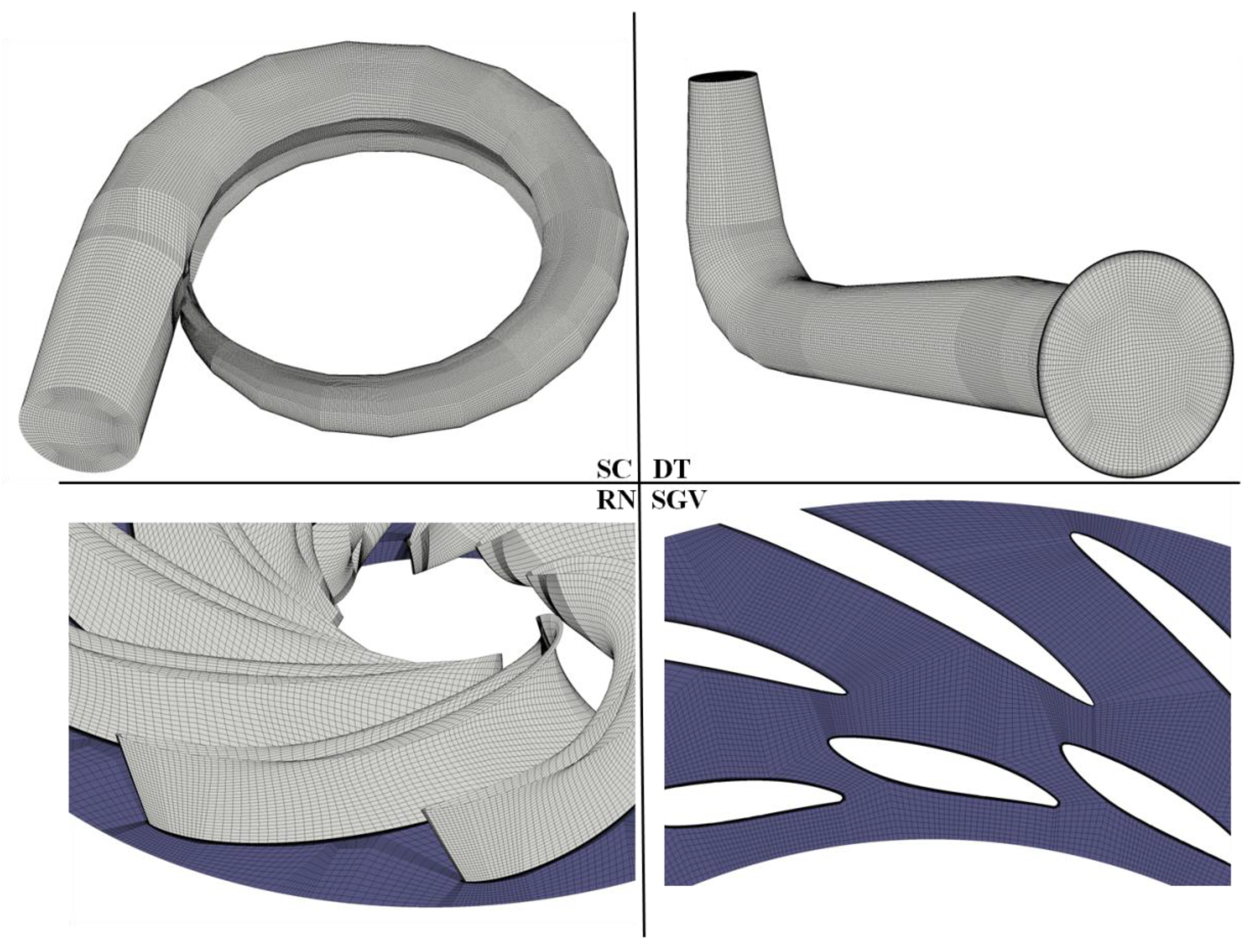
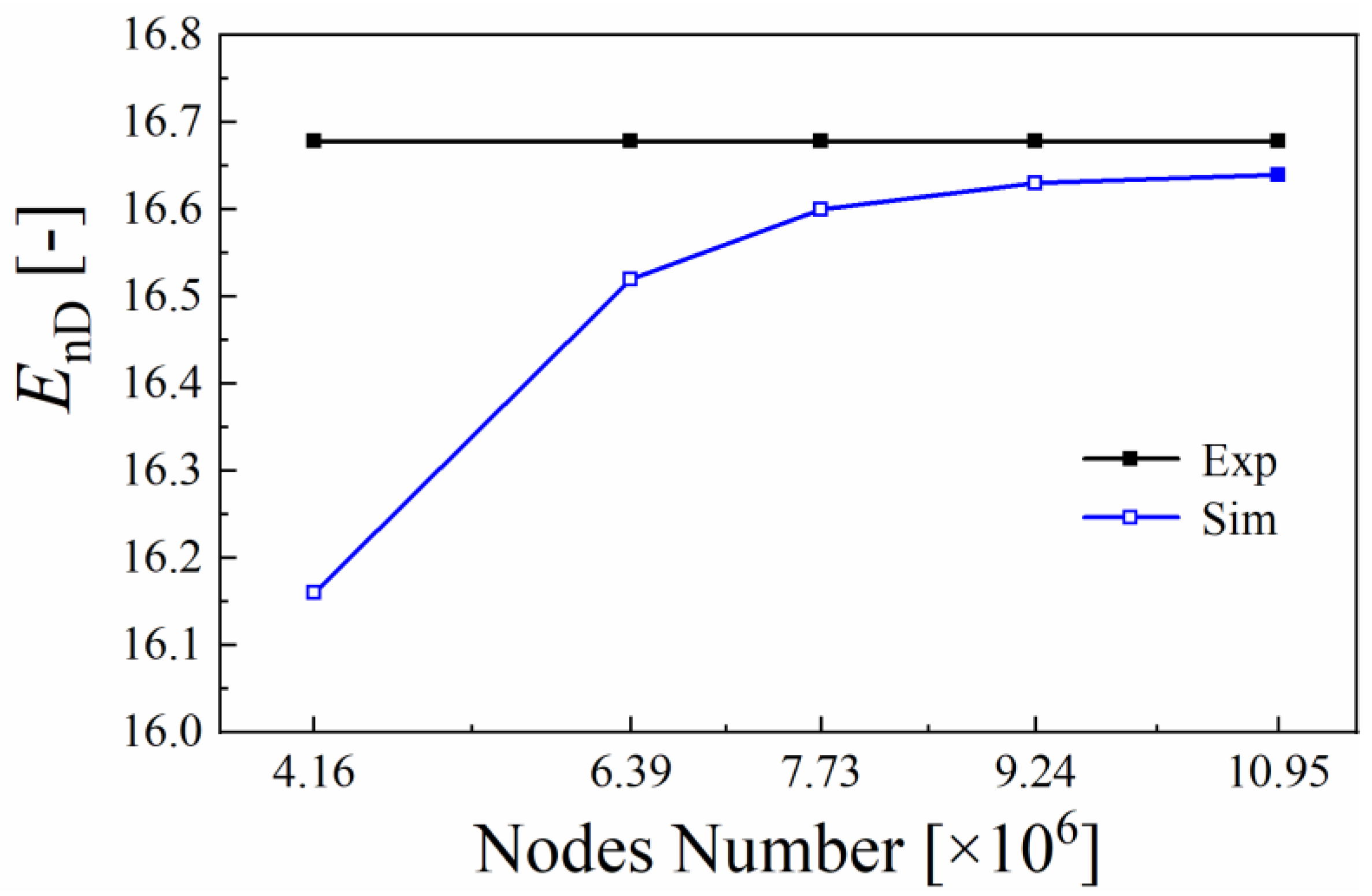
2.3. Grid Generation and Independence Validation

Figure 3 shows the generated structure grid in the four fluid domains. For all flow domains except the spiral casing region, y+ of the boundary layer was less than 2, which is sufficient for the following numerical simulation.

For grid independence validation, five grids with 4.16 × 10⁶, 6.39 × 10⁶, 7.73 × 10⁶, 9.24 × 10⁶, and 10.95 × 10⁶ nodes were generated. The detailed information of these five sets of grids is listed in

Table 2. Detailed grid information (million).

Domain	1st	2nd	3rd	4th	5th
Draft tube	0.57	1.03	1.32	1.69	2.09
Runner	1.83	2.29	2.75	3.20	3.56
Guide/stay vane	1.17	1.95	2.34	2.80	3.26
Spiral casing	0.59	1.12	1.32	1.55	2.04
Total	4.16	6.39	7.73	9.24	10.95

. Since hump performance is our investigation object, the head value at best efficiency point 1.00Q_BEP was selected as the criteria of grid independence. Figure 4 reveals that, when the total number of nodes increased from 7.73 × 10⁶ to 10.95 × 10⁶, the variation of the head value was within 0.5%. Accordingly, the grid with 10.95 × 10⁶ nodes was selected in the present paper for all simulations.

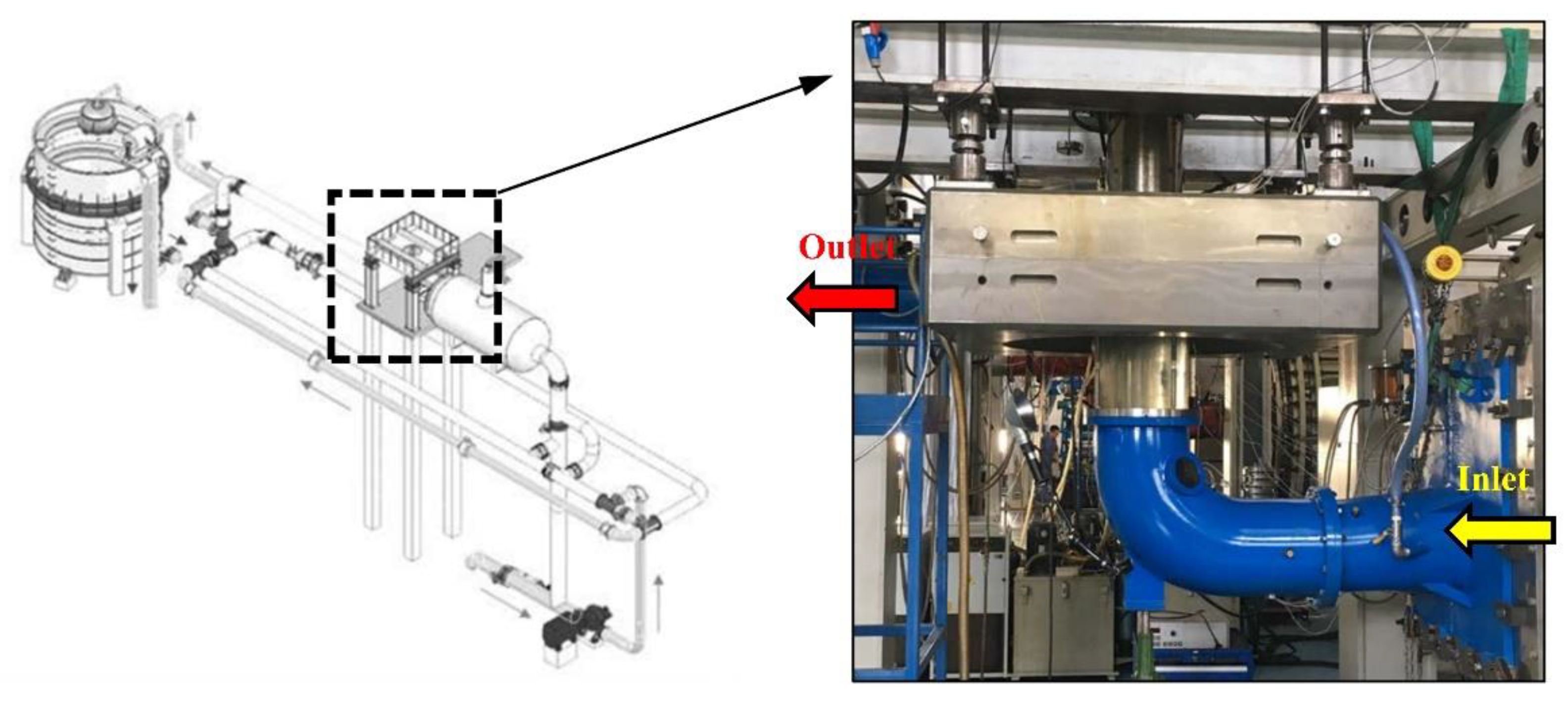
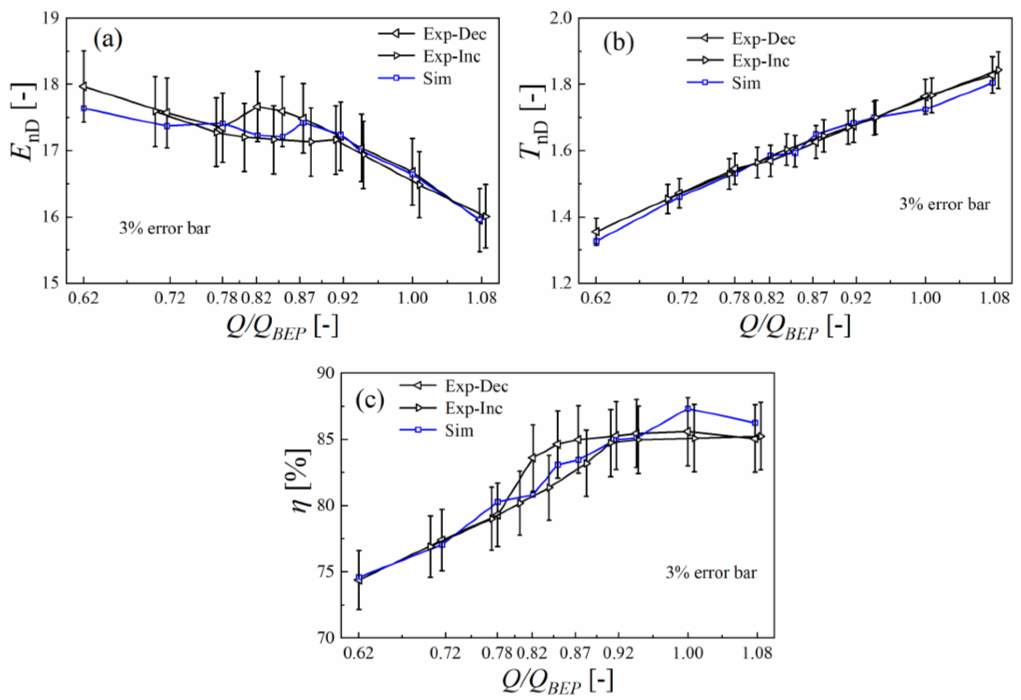
3. Experimental Setup and Validation

The hydraulic performance (energy characteristic, torque characteristic, and efficiency) of the original runner was tested in the test rig (shown in Figure 5) of Harbin Institute of Large Electrical Machinery (HILEM). The max head and the max flow rate of the experimental setup were 80 m and 0.8 m³/s, respectively. The efficiency random uncertainty was within 0.050%, and the final comprehensive efficiency uncertainty of the test rig was $\pm 0.198\%$, both of which completely meet the standard of the IEC (International Electrotechnical Commission).

To evaluate the accuracy of the performed simulations, the obtained energy performance, torque performance, and efficiency performance from experimental data were compared with that from the simulation results, and the results are shown in Figure 4, of which, the energy factor, torque factor, and efficiency are defined in Equations (2) and (4).

$$E_{nD}=\frac{gH}{n_{}^2{D}_1^2}$$

(2)

$$T_{nD}=\frac{T}{\rho n_{}^2{D}_1^5}$$

(3)

$$\eta =\frac{\rho gQH}{\omega T}\times 100\%$$

(4)

where $g$ is local gravity acceleration, 9.8 m/s²; n is rotational speed of the runner, rpm; H is the head, m; D₁ is the runner inlet diameter in pump mode, m; T is torque, N m; and $\omega$ is angular velocity, rad/s.

It was found that, in the experiment, the energy characteristic performed differently in the discharge increase and decrease directions. This phenomenon is known as the hysteresis characteristic. It is proven that only numerical calculation with initial conditions obtained from neighboring discharge operation points could reproduced this phenomenon [6]. To avoid the influence of the hysteresis characteristics, all numerical simulations were conducted without initial conditions. Figure 6 reveals that the relative errors of all simulated performance characteristics were less than 3%.

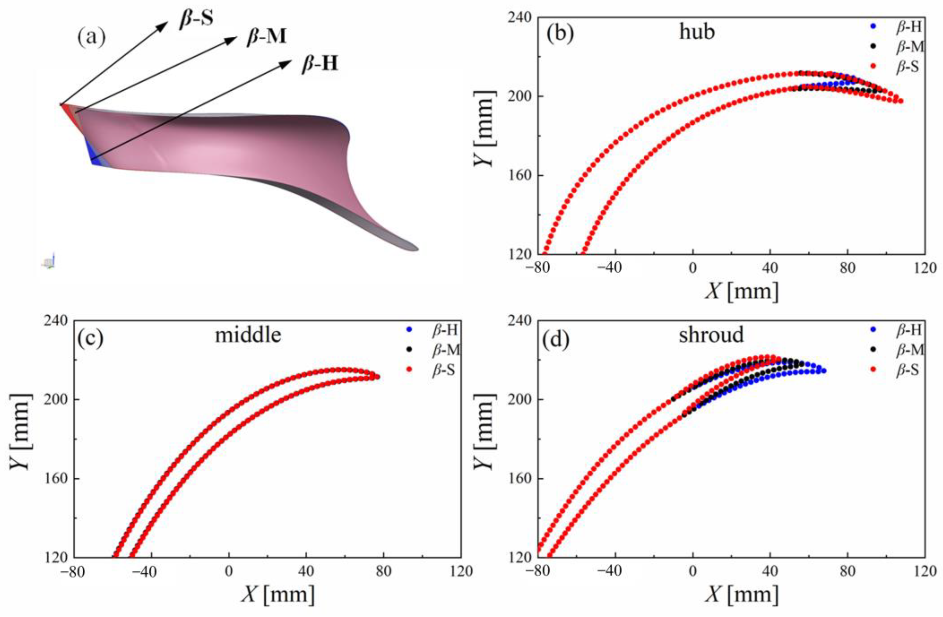
4. Setting Angle Distribution Plans

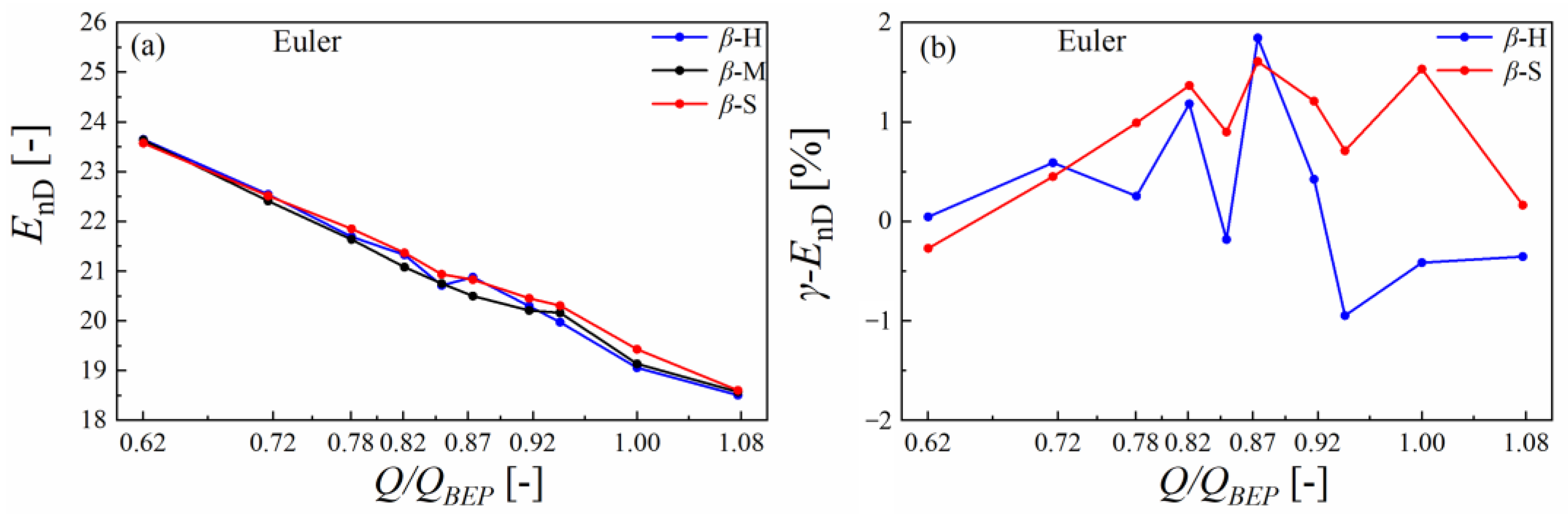
4.1. Euler Head Analysis

The hump characteristic is a typical unsteady characteristic, and it can be observed in the energy-discharge curve. Equation (4) indicates that the energy-discharge characteristic can be considered as the combined action of the Euler head and the hydraulic loss. In the design stage, a no swirling ($C_{u1}$ = 0) condition is assumed at the runner inlet so the theoretical Euler head can be re-written as Equation (6). Runner outlet radius (R₂), discharge Q, guide vane height B₀, and rotational speed $\omega$ could be assumed as constants, hence the Euler head value only depends on the relative flow angle (β₂). In most publications and in traditional design, the setting angle (β₂) at the runner outlet remains unchanged; however, asymmetric complex flow has been observed when the pump turbine strays into the hump region. Moreover, the previous theory could not show a clear relationship between design parameters and hump performance. Accordingly, it is significant to investigate the influence of setting angle distribution on hump performance.

$$H_{net}=H_{Euler}-H_{loss}$$

(5)

$$H_E{}_{uler}=\frac{\Delta C_u\cdot U}{g}=\frac{C_{u2}\cdot U_2-C_{u1}\cdot U_1}{g}=\frac{U_{{}_2}^2-U_{{}_1}^2}{g}-\frac{Q\omega }{g}(\frac{R_2}{A_2\tan {\beta }_{{}_2}^{}}-\frac{R_1}{A_1\tan {\beta }_1^{}})$$

(6)

$$H_E{}_{uler}=\frac{{\omega }^2}{g}\cdot R_{{}_2}^2-\frac{\omega }{2\pi g{B}_0}\cdot \frac{Q}{\tan {\beta }_{{}_2}^{}}=C{\mathit{onst}}_1-C{\mathit{onst}}_2\cdot \frac{1}{\tan {\beta }_{{}_2}^{}}$$

(7)

where ΔC_u·U is the Euler momentum (the change of velocity momentum), m²·s⁻²; A₁, A₂ are runner inlet area and runner outlet area, respectively, m²; U₁, U₂ are circumferential velocity at runner inlet and outlet, respectively, in pump mode, m·s⁻¹; n is the rotational speed of the runner, rpm; H is the head, m; B₀ is the guide vane height, m; β₂ is the relative flow angle at the runner outlet in pump mode; and Q is the discharge, m³·s.

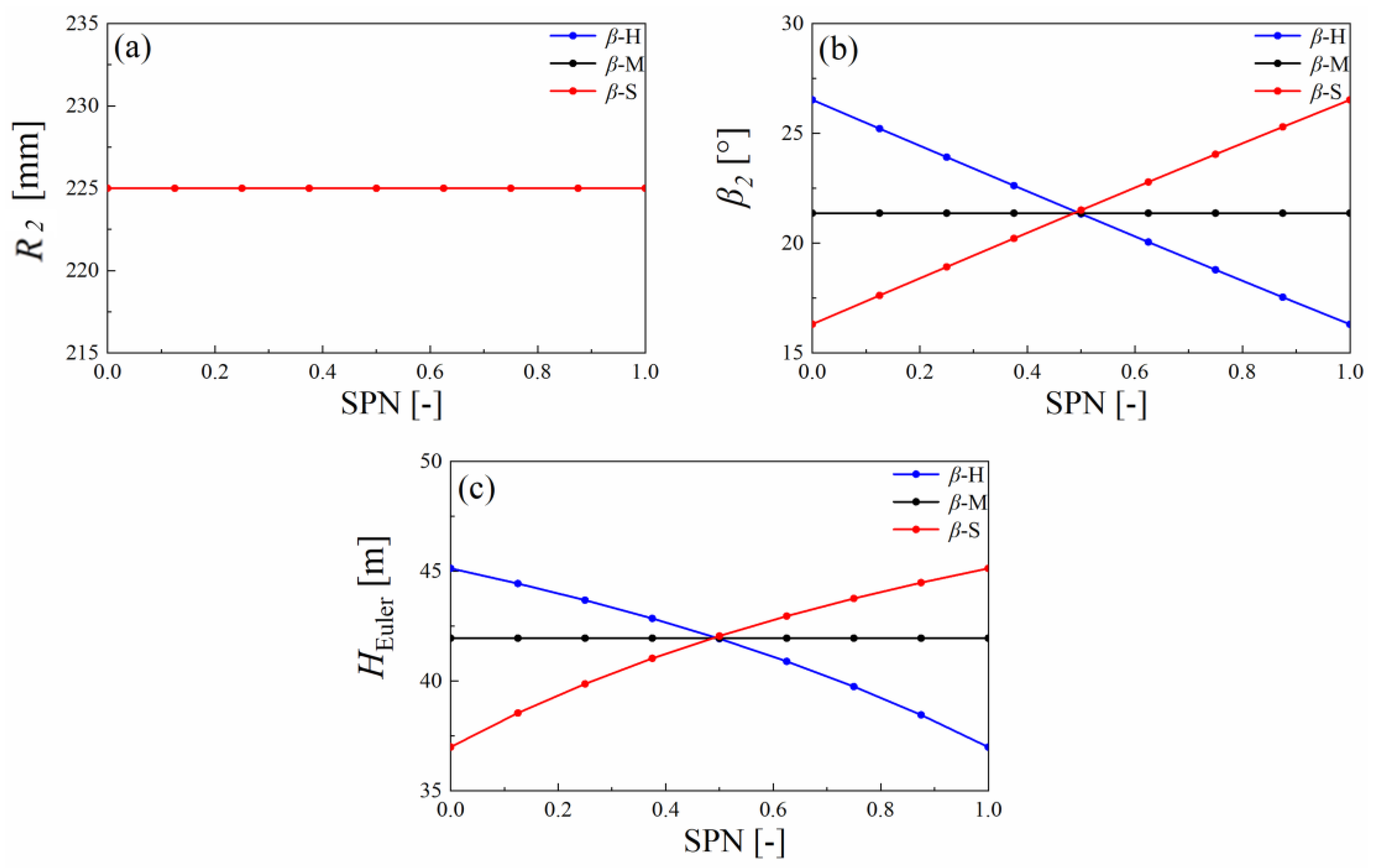
4.2. Setting Angle Distribution Plans at the Runner Outlet

In this section, three runners with different setting angle distribution plans are proposed. β-S, β-M, and β-H refer to three runners with different distribution rules for the setting angle at the runner outlet. The detailed parameters of these three runners are shown in Figure 7, of which plan β-M the is a control plan, and its setting angle is distributed evenly in the spanwise direction of the runner outlet. β-S and β-H refer to two innovative runners proposed in our paper, whose setting angle is distributed linearly in the spanwise direction of runner outlet while showing different distribution rules. For plan β-S, the setting angle follows a linear growth law from the hub to the shroud side, while plan β-H shows a completely opposite linear distribution rule. Moreover, the geometry of these three runners is modeled and compared in Figure 8.

5. Results and Discussions

The definition of relative change rate is shown in Equation (7), where $\phi$ is the comparison parameter, which can be replaced by energy factor, torque factor, and efficiency.

$$\gamma =({\phi }_i-{\phi }_M)/{\phi }_M\times 100\%$$

(8)

5.1. Analysis of the Performance Characteristics

Figure 9 depicts the hydraulic characteristic comparison among three different setting angle distribution plans. It can be seen that different distribution plans show different energy-discharge characteristics, especially in the hump region. Compared with plan β-H, the valley point in plan β-M and plan β-S moved to smaller operating points, and plan β-S could enlarge the hump margin. Compared with plan β-M, plan β-H increased the energy factor at discharge operation points over 0.72 Q_BEP while plan β-S decreased the energy factor in discharge operation points less than 0.92Q_BEP, which means that both plan β-H and plan β-S can effectively increase the energy factor in the hump region. The hump characteristics improvement comparison between our case and other published papers is shown in

Table 3. Hump characteristics improvement comparison.

Ref.	Method	Original Energy Factor at Hump Valley	Optimized Energy Factor at Hump Valley	Relative Improvement Rate/%
[25]	Bio-inspired leading-edge protuberances	0.013625	0.014	2.75
		0.013625	0.01417	4
[19]	Groove method	1.068	1.088	1.87
Our case	Runner outlet	17.18	17.262 (plan β-S)	0.48
		17.18	17.209 (plan β-H)	0.17

. Even if the relative improvement rate in our case is not as large as the relative improvement rate in other papers, the hump margin in plan β-S increased from 4% to 4.5% compared with the hump margin in the original runner β-M, which fully meets the engineering standard. Moreover, compared to other methods, optimization of the runner outlet is more likely to be achieved in the design stage and be applied in engineering applications.

For the torque characteristic, when compared with plan β-M, plan β-S increased the torque factor of nearly all discharge operating points, while plan β-H just increased the torque factor at some specific discharge operating points in the hump region and decreased the torque factor in the discharge operating points over 0.92 Q_BEP.

When it comes to efficiency characteristics, it can be seen that plan β-H and plan β-S played opposite roles for the operating points apart from the hump region. Plan β-H can significantly increase the efficiency at discharge operation points over 0.8 Q_BEP while decreasing the efficiency at discharge operation points less than 0.7 Q_BEP. By contrast, plan β-S mainly increased the efficiency at discharge operation points less than 0.78 Q_BEP, whereas it decreased the efficiency at discharge operation points over 0.85 Q_BEP.

It is known that the Euler head (the input energy), as well as the hydraulic loss, is the main cause of the hump performance; hence, the effect of different setting angle distribution plans on the Euler head and hydraulic loss will be analyzed in the following sections.

5.2. Comparative Analysis on Euler Head

Figure 10 shows the distributions of the Euler head in different plans, and it can be seen that the Euler head in plan β-S was increased compared to that in plan β-M, and the improvement degree was within 1.6%. On the other hand, plan β-H could only raise the Euler head at some specific operating points in the hump region. Moreover, for plan β-H, the Euler head suddenly dropped at 0.85 Q_BEP, corresponding to the same discharge operating point that the valley point appears at in its energy-discharge curve. Hence, the sudden drop of the Euler head is attributed as the reason causing the hump characteristics in plan β-H. It should be noted that the spanwise-averaged Euler head in the three runners was the same theoretically, while the CFD results show that the mass-flow-averaged Euler head under different plans in the three-dimensional flow field was quite different, indicating that the setting angle distribution at the runner outlet can significantly affect the flow characteristics in the spanwise direction. However, this effect cannot be clearly explained by Equation (5). To resolve this shortcoming, Equation (9) was adopted to express the Euler head in the three-dimensional flow field. It is known that the Euler head is a function of the absolute flow angle α₂. The comparisons of absolute flow angle α₂ distribution in the spanwise and circumferential directions are investigated in the following section. Moreover, four typical discharge operation points, including 0.78 Q_BEP, 0.82 Q_BEP, 0.87 Q_BEP, and 1.00 Q_BEP were chosen.

$$H_E{}_{uler}=\frac{\Delta C_{u}U}{g}=\frac{C_{u2}{U}_2-C_{u1}{U}_1}{g}\approx \frac{T\omega }{gQ}$$

(9)

$$H_E{}_{uler}=\frac{\Delta C_{u}U}{g}=\frac{C_{u2}{U}_2-C_{u1}{U}_1}{g}=\frac{Q{U}_2}{g\tan {\alpha }_2{A}_2}$$

(10)

where ΔC_u·U is the Euler momentum (the change of velocity momentum), m²·s⁻²; U₁, U₂ are circumferential velocity at runner inlet and outlet, respectively in pump mode, m·s⁻¹; $\omega$ is angular velocity, rad/s; α₂ is the absolute flow angle at the runner outlet in pump mode; Q is the discharge, m³·s; $g$ is local gravity acceleration, 9.8 m/s²; A₂ is the runner inlet area, m²; and T is torque, N m.

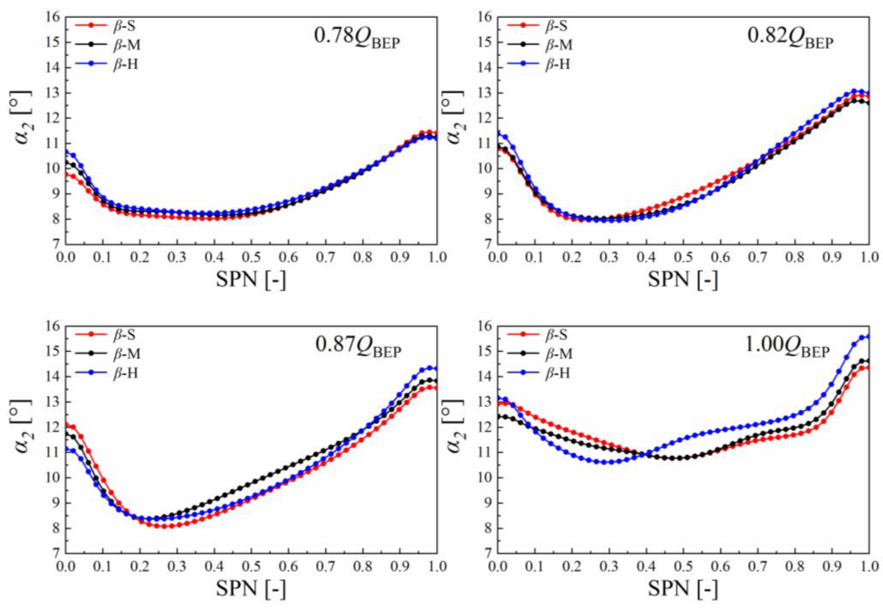
5.2.1. Absolute Flow Angle in Spanwise Direction

Figure 11 illustrates the distributions of the mass-flow-averaged absolute flow angle α₂ along the spanwise direction at the runner outlet. It can be seen that setting angle distribution significantly affected the absolute flow angle α₂ distribution at the investigated operating points. At 1.00 Q_BEP, the distribution of the absolute flow angle α₂ at the runner outlet was highly consistent with the theoretical setting angle distribution plans: the position with a large setting angle β₂ tends to have a small absolute flow angle and vice versa. With the decrease of discharge, the differences of the absolute flow angle α₂ distribution under the three plans became smaller. At 0.87 Q_BEP, the smallest absolute flow angle was achieved in plan β-S in the SPN0.2–SPN1.0 region, and the largest absolute flow angle was obtained in plan β-M in the SPN0.3–SPN0.7 region in the spanwise direction at the runner outlet. When it comes to 0.82 Q_BEP, the absolute flow angle in plan β-S was the largest in the middle of the spanwise direction (about SPN0.4–SPN0.8), while plan β-H provided the largest absolute flow angle for the rest region in the spanwise direction. At 0.78 Q_BEP, the difference of the absolute flow angle distribution under the three plans could only be distinguished at the hub region where the absolute flow angle in plan β-S was smaller than that in the other two plans.

5.2.2. Absolute Flow Angle in Circumferential Direction

The absolute flow angle value in the specific spanwise direction can be defined as the circumferential-averaged value of the absolute flow angle. Therefore, it is necessary to investigate the absolute flow angle distribution in the circumferential direction. Figure 12 shows the comparison of absolute flow angle α₂ distributions in the circumferential direction under three different plans. In this section, three typical planes from hub to shroud in the spanwise direction were selected and marked as SPN0.2, SPN0.5, and SPN0.8. In 1.00 Q_BEP, the absolute flow angle in the plan β-H was the smallest and plan β-S provided the larger absolute flow angle in most regions in the circumferential direction, which is consistent with the theoretical design. However, when it comes to the operating points in the hump region, the differences of absolute flow angle α₂ distribution in the circumferential direction under the three different plans could hardly be distinguished, indicating that the influence of different setting angle distribution plans on absolute flow angle distribution in the circumferential direction was not large enough to be captured; only in the circumferentially averaged method can the influence be distinguished.

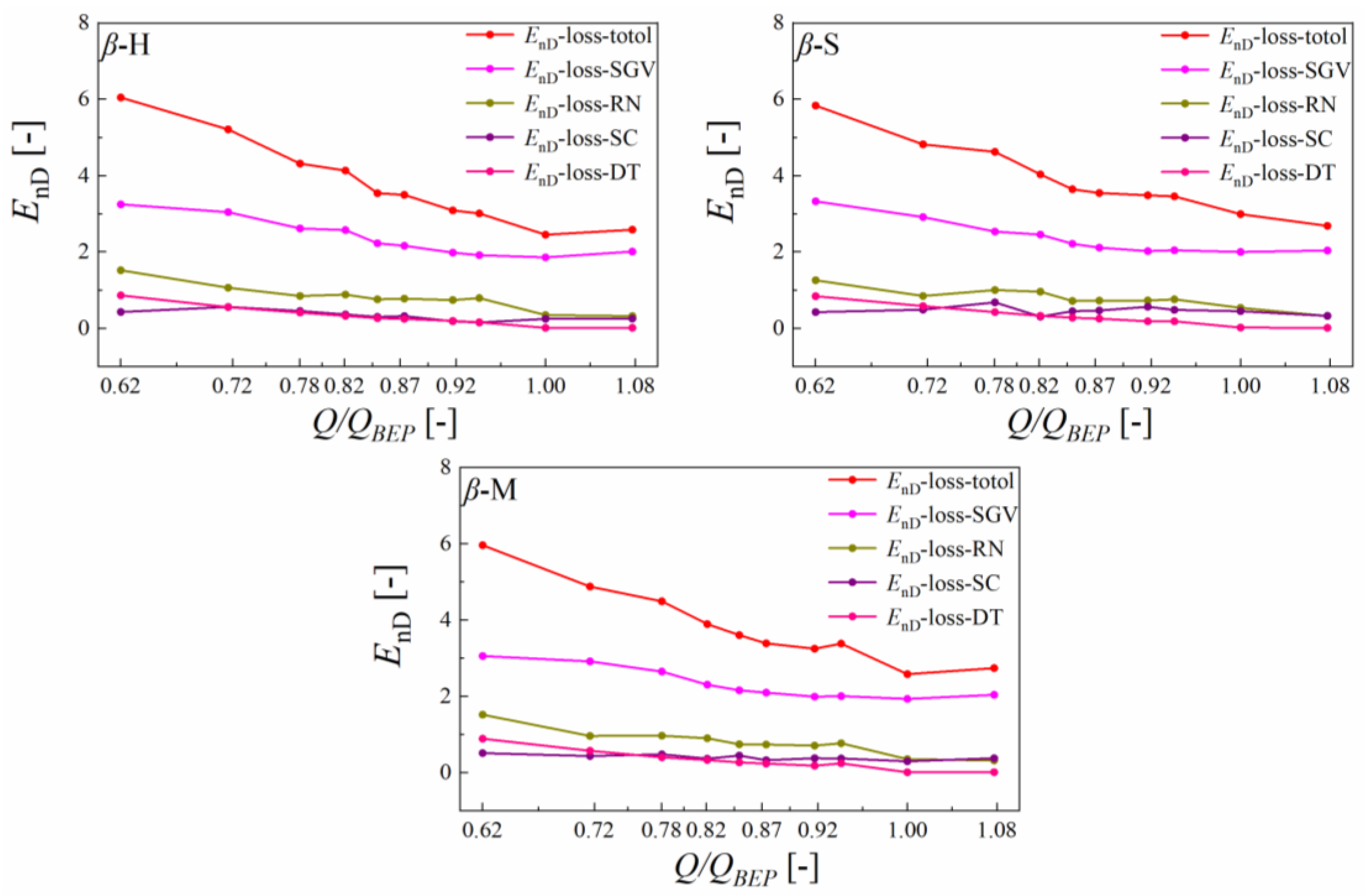
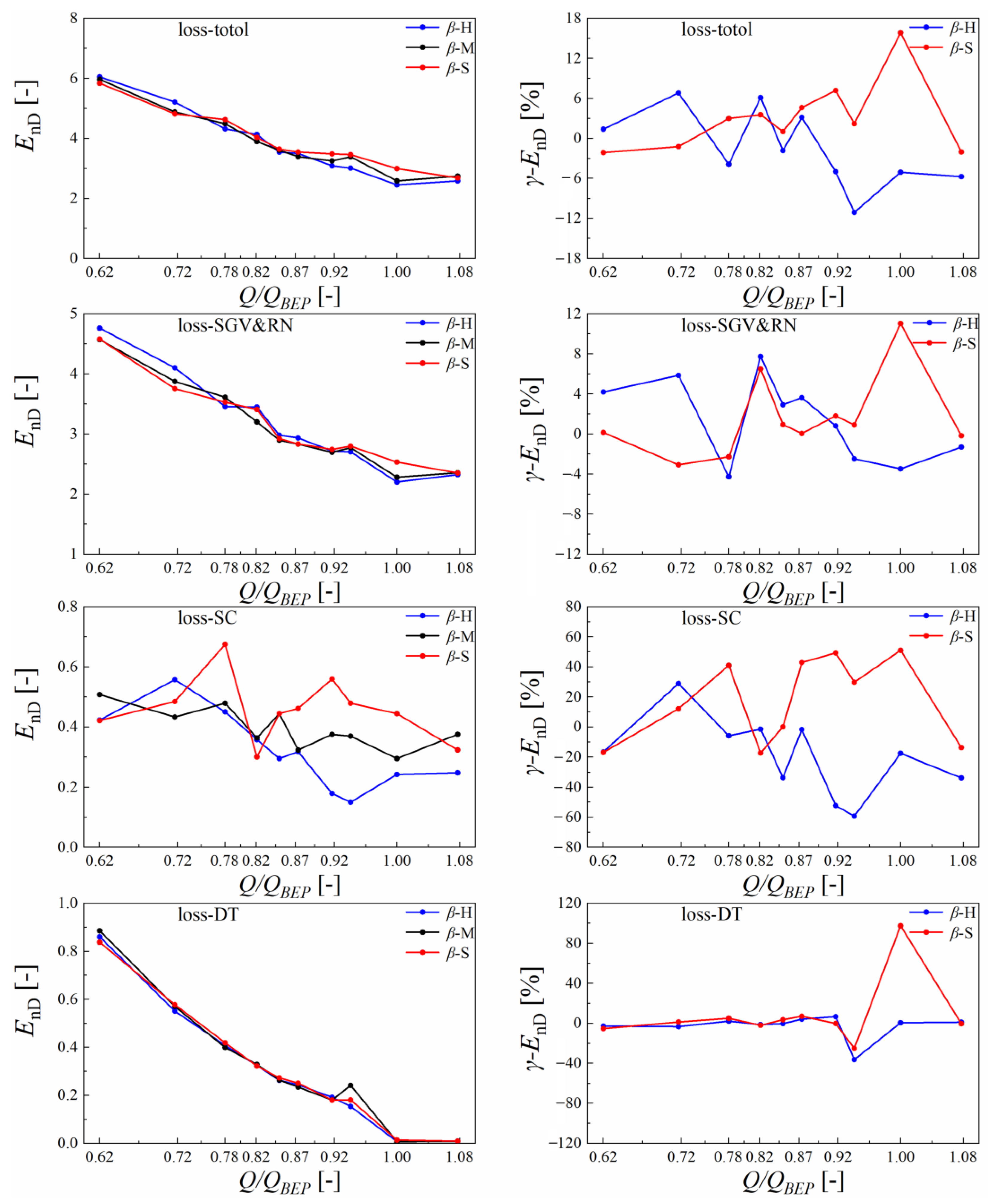
5.3. Hydraulic Loss Comparation

The hydraulic loss comparison among these three plans is shown in Figure 13. It can be seen that, for all plans, the proportion as well as the variation trend of the hydraulic loss in each flow domain remain unchanged. Generally, the hydraulic loss in the stay/guide vanes takes up the largest portion, and the hydraulic loss in the runner domain takes the second place. Meanwhile, the hydraulic loss in the remaining flow domains (spiral casing domain and the draft tube) has a negligible share in the total hydraulic loss.

Figure 14 shows the effect of the setting angle distribution on the hydraulic loss in each flow domain. It can be seen that the variation trend of the hydraulic loss in the SGV &RN region was exactly the same as the total hydraulic loss, indicating that different setting angle distribution mainly affected the distribution of the hydraulic loss in the SGV &RN region, thereby affecting the total hydraulic loss.

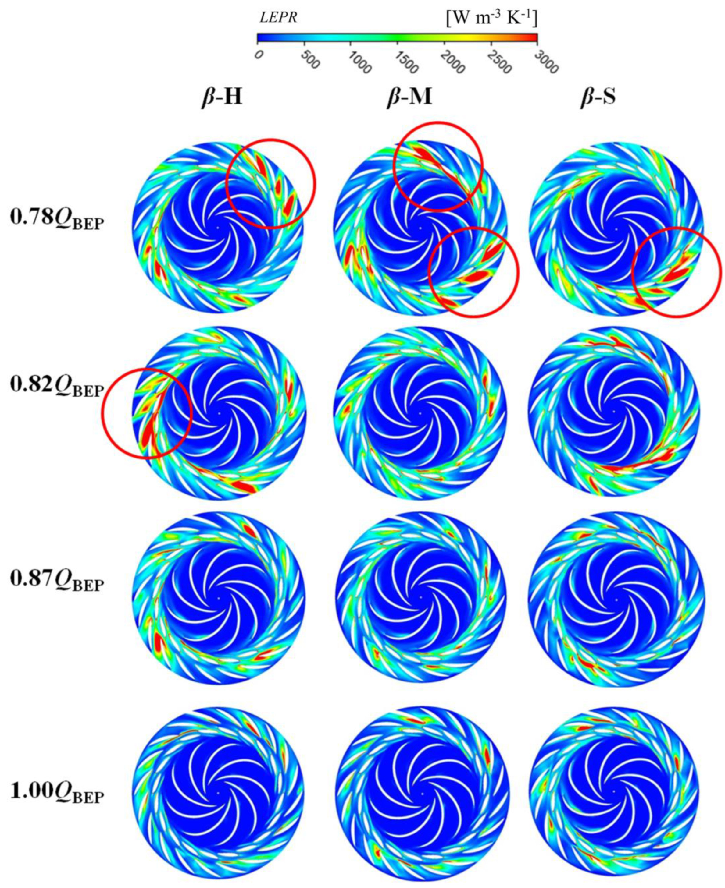
Hydraulic Loss Distribution Analysis

In this section, the influence of the setting angle distribution on the hydraulic loss distribution in the flow domain is investigated in detail. Recently, the local entropy production rate (LEPR) method, proposed in previously published papers [26], has been proven to be accurate and practical enough to describe the position and level of hydraulic loss in hydraulic machinery. Hence, the LEPR method was employed to depict hydraulic loss distribution in the stay/guide vane domain as well as the runner domains.

Figure 15 shows the local hydraulic loss distribution in typical spanwise planes at selected discharge operating points. It was observed that at 1.00 Q_BEP, the distribution of the LEPR under the three runners was nearly the same and was hard to distinguish. However, when the discharge decreased to 0.87 Q_BEP, a high-LEPR region was formed in the stay/guide vanes channels, and the high-LEPR area in plan β-H was much larger than that in the other two distribution plans. When the discharge operating point continued to decrease from 0.87 Q_BEP to 0.82 Q_BEP, the high-LEPR region was enlarged under all these three plans and even expanded to the vaneless region. During this process, the increase of high LEPR was most severe in plan β-H when compared to plan β-M and plan β-S, resulting in the hump characteristic of plan β-H at 0.82Q_BEP. With the discharge further decreased to 0.78Q_BEP, the size of the high-LEPR area continued increasing under all these three distribution plans, and the increase level of LEPR in β-M and plan β-S was much larger than that in plan β-H, resulting in the hump characteristic in both plan β-M and plan β-S at 0.78Q_BEP. It needs to be pointed out that, although plan β-M and plan β-S share the same valley point (0.78Q_BEP) in the hump region, the size of the high-LEPR region in plan β-M was much larger than that in plan β-S, resulting in a larger hump safety margin in plan β-S.

6. Conclusions

In the present paper, the optimization of setting angle distribution to suppress hump characteristic in pump turbine was investigated numerically. Based on the numerical results, the following conclusions were obtained:

(1)

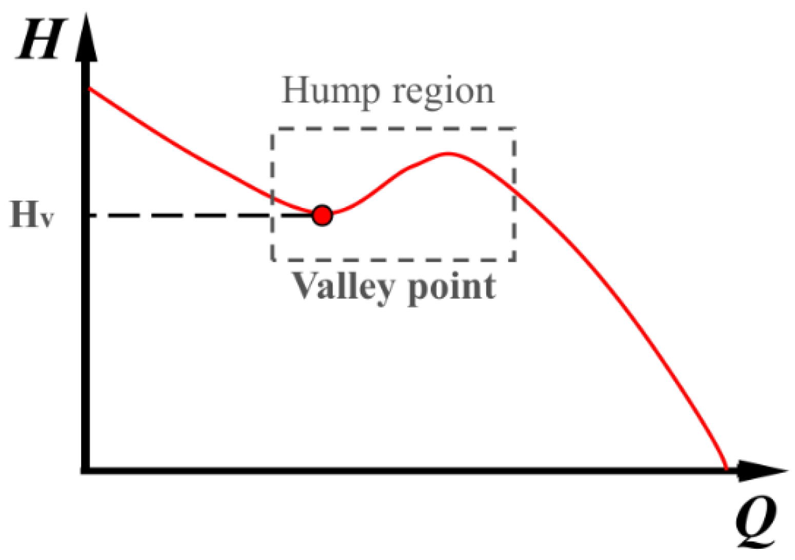
The hump characteristic is related to the setting angle distribution at the runner the outlet; however, the influence of setting angle distribution cannot be captured through conventional design methods and the Euler head theory. This can be attributed to the limitations of two-dimensional theory (conventional design methods and Euler head theory) when investigating the hump region.

(2)

In the different setting angle distribution plans, the runner whose setting angle at the shroud was 10° larger than that at the hub effectively increased the hump margin from 4% to 4.5% compared to the original runner β-M, which fully meets the engineering standard. Moreover, compared to other hump-region-elimination methods proposed by related papers, optimization of the runner outlet is more likely to be achieved in the design stage and applied in engineering applications.

(3)

Setting angle distribution at the runner outlet could affect the absolute flow angle α₂ distribution in the spanwise direction as well as the hydraulic loss spatial distribution in the hump region, contributing to different hump performances under different plans.

Based on the current research, it is necessary to perform unsteady simulations using the best distribution plan to study the unsteady characteristics in the vaneless region.

References

1. Zuo, Z.G.; Fan, H.G.; Liu, S.H.; Wu, Y. S-shaped characteristics on the performance curves of pump-turbines in turbine mode-a review. Renew. Sustain. Energy Rev. 2016, 60, 836–851. [Google Scholar] [CrossRef]
2. Gentner, C.; Sallaberger, M.; Widmer, C.; Braun, O.; Staubli, T. Numerical and experimental analysis of instability phenomena in pump turbines. IOP conference series. Earth Environ. Sci. 2019, 15, 32042. [Google Scholar]
3. Jia, J.; Zhang, J.F.; Qu, Y.F.; Cai, H.; Chen, S. Study on hump characteristics of pump turbine with different guide vane exit angles. IOP conference series. Earth Environ. Sci. 2019, 240, 72038. [Google Scholar]
4. Ješe, U.; Fortes-Patella, R.; Dular, M. Numerical study of pump-turbine instabilities under pumping mode off-design conditions. In Proceedings of the ASME-JSME-KSME 2015 Joint Fluids Engineering Conference, Seoul, Reoublic of Korea, 26–31 July 2015. [Google Scholar]
5. Yangyang, Y.; Yexiang, X.; Wei, Z.; Liming, Z.; Hwang, A.S.; Zhengwei, W. Numerical analysis of a model pump-turbine internal flow behavior in pump hump district. IOP conference series. Earth Environ. Sci. 2014, 22, 32040. [Google Scholar]
6. Li, D.; Wang, H.; Qin, Y.; Han, L.; Wei, X.; Qin, D. Entropy production analysis of hysteresis characteristic of a pump-turbine model. Energy Convers. Manag. 2017, 149, 175–191. [Google Scholar] [CrossRef]
7. Qin, Y.; Li, D.; Wang, H.; Liu, Z.; Wei, X.; Wang, X. Investigation on hydraulic loss component and distribution in hydraulic machinery: A case study of pump-turbine in pump mode. J. Energy Storage 2022, 52, 104932. [Google Scholar] [CrossRef]
8. Qin, Y.; Li, D.; Wang, H.; Liu, Z.; Wei, X.; Wang, X. Investigation on the relationship between hydraulic loss and vortex evolution in pump mode of a pump-turbine. J. Hydrodyn. 2022, 34, 555–569. [Google Scholar] [CrossRef]
9. Li, D.; Chang, H.; Zuo, Z.; Wang, H.; Li, Z.; Wei, X. Experimental investigation of hysteresis on pump performance characteristics of a model pump-turbine with different guide vane openings. Renew. Energy 2020, 149, 652–663. [Google Scholar] [CrossRef]
10. Ran, H.J.; Luo, X.W.; Chen, Y.L.; Xu, H.Y.; Farhat, M. Hysteresis phenomena in hydraulic measurement. IOP conference series. Earth Environ. Sci. 2012, 15, 62048. [Google Scholar]
11. Li, D.; Song, Y.; Lin, S.; Wang, H.; Qin, Y.; Wei, X. Effect mechanism of cavitation on the hump characteristic of a pump-turbine. Renew. Energy 2021, 167, 369–383. [Google Scholar] [CrossRef]
12. Anciger, D.; Jung, A.; Aschenbrenner, T. Prediction of rotating stall and cavitation inception in pump turbines. IOP conference series. Earth Environ. Sci. 2010, 12, 12013. [Google Scholar]
13. Liu, J.; Liu, S.; Wu, Y.; Jiao, L.; Wang, L.; Sun, Y. Numerical investigation of the hump characteristic of a pump-turbine based on an improved cavitation model. Comput. Fluids 2012, 68, 105–111. [Google Scholar] [CrossRef]
14. Yang, W.; Xiao, R.F. Multiobjective optimization design of a Pump-Turbine impeller based on an inverse design using a combination optimization strategy. J. Fluids Eng. 2014, 136, 145011–145019. [Google Scholar] [CrossRef]
15. Olimstad, G.; Nielsen, T.; Børresen, B. Dependency on runner geometry for Reversible-Pump turbine characteristics in turbine mode of operation. J. Fluids Eng. 2012, 134, 1211021–1211029. [Google Scholar] [CrossRef]
16. Zhu, B.; Tan, L.; Wang, X.; Ma, Z. Investigation on flow characteristics of Pump-Turbine runners with large blade lean. J. Fluids Eng. 2018, 140, 031101. [Google Scholar] [CrossRef]
17. Zhu, B.; Wang, X.; Tan, L.; Zhou, D.; Zhao, Y.; Cao, S. Optimization design of a reversible pump-turbine runner with high efficiency and stability. Renew. Energy 2015, 81, 366–376. [Google Scholar] [CrossRef]
18. Ran, H.; Luo, X.; Zhang, Y.; Zhuang, B.; Xu, H. Numerical simulation of the unsteady flow in a High-Head pump turbine and the runner improvement. In Proceedings of the ASME 2008 Fluids Engineering Division Summer Meeting collocated with the Heat Transfer, Energy Sustainability, and 3rd Energy Nanotechnology Conferences, Jacksonville, FL, USA, 10–14 August 2008. [Google Scholar]
19. Liu, Y.; Ran, H.J.; Wang, D.Z. Research on groove method to suppress stall in pump turbine. Energies 2020, 13, 3822. [Google Scholar] [CrossRef]
20. Xue, P.; Liu, Z.P.; Lu, L.; Tian, Y.J.; Wang, X.; Chen, R. Research and optimization of performances of a pump turbine in pump mode. IOP Conf. Ser. Earth Environ. Sci. 2012, 240, 72012. [Google Scholar] [CrossRef]
21. Li, D.Y.; Gong, R.Z.; Wang, H.J.; Wei, X.Z.; Liu, Z.S.; Qin, D.Q. Unstable head-flow characteristics of pump-turbine under different guide vane openings in pump mode. J. Drain. Irrig. Mach. Eng. 2016, 34, 1–8. (In Chinese) [Google Scholar]
22. Ren, Z.; Hao, H.; Li, D.; Wang, H.; Liu, J.; Li, Y. Dissolution and evolution effects on pressure fluctuations in a space micropump. Proc. Inst. Mech. Eng. Part E J. Process Mech. Eng. 2022. [Google Scholar] [CrossRef]
23. Cavazzini, G.; Covi, A.; Pavesi, G.; Ardizzon, G. Analysis of the unstable behavior of a Pump-Turbine in turbine mode: Fluid-Dynamical and spectral characterization of the s-shape characteristic. J. Fluids Eng.-Trans. ASME 2015, 138, 21105. [Google Scholar] [CrossRef]
24. ANSYS Inc. ANSYS CFX-Solver Theory Guide; ANSYS Inc.: Canonsburg, PA, USA, 2018. [Google Scholar]
25. Zhiwei, G.; Chihang, W.; Zhongdong, Q.; Xianwu, L.; Weipeng, X. Suppression of hump characteristic for a pump-turbine using leading-edge protuberance. Proc. Inst. Mech. Eng. Part A J. Power Energy 2020, 234, 187–194. [Google Scholar] [CrossRef]
26. Pei, J.; Meng, F.; Li, Y.; Yuan, S.; Chen, J. Effects of distance between impeller and guide vane on losses in a low head pump by entropy production analysis. Adv. Mech. Eng. 2016, 8, 2071837044. [Google Scholar] [CrossRef] [Green Version]
Figure 1. Configuration of the pump turbine model.
Energies 16 02471 g001aEnergies 16 02471 g001b
Figure 2. Description of the hump region.
Energies 16 02471 g002
Figure 3. Grids detailed information.
Energies 16 02471 g003
Figure 4. Grid independence at the best efficiency point of 13 mm GVO.
Energies 16 02471 g004
Figure 5. Scheme of the test rig in HILEM.
Energies 16 02471 g005
Figure 6. Experimental verification: (a) energy, (b) torque, (c) efficiency.
Energies 16 02471 g006
Figure 7. Distributions of design parameters in different runners along the spanwise direction: (a) R2, (b) β2, (c) HEuler.
Energies 16 02471 g007
Figure 8. Blade geometry comparison in typical planes: (a) blade geometric modeling, (b) hub, (c) middle, and (d) shroud.
Energies 16 02471 g008
Figure 9. The performance characteristics and relative change rates of various plans: (a,b) energy, (c,d) torque, (e,f) efficiency.
Energies 16 02471 g009
Figure 10. Distribution of Euler head at different plans and relative change rates.
Energies 16 02471 g010
Figure 11. Distributions of the absolute flow angle α2 in the spanwise direction at the runner outlet at typical discharge operation points.
Energies 16 02471 g011
Figure 12. Distributions of absolute flow angle α2 at the runner outlet in the circumferential direction.
Energies 16 02471 g012
Figure 13. Distribution of hydraulic loss in 13 mm GVO.
Energies 16 02471 g013
Figure 14. Distribution and relative change rate of hydraulic loss.
Energies 16 02471 g014
Figure 15. Comparison of hydraulic loss distribution in middle spanwise plane in discharge operation points.
Energies 16 02471 g015