Article

Coupled Electromagnetic–Thermal Modelling of Dynamic Performance for Modular SPM Machines

1
Electrical Machines & Drives Group, Department of Electronic and Electrical Engineering, University of Sheffield, Sheffield S10 2TN, UK
2
Motor Design Ltd., An Ansys Company, 5 Edison Court, Wrexham LL13 7YT, UK
*
Author to whom correspondence should be addressed.
Energies 2023, 16(6), 2516; https://doi.org/10.3390/en16062516
Submission received: 30 January 2023 / Revised: 22 February 2023 / Accepted: 5 March 2023 / Published: 7 March 2023

Abstract

:
This paper presents coupled electromagnetic (EM)–thermal modelling of the steady-state dynamic performances, such as torque speed curve and the efficiency map, for surface-mounted permanent magnet machines. One important feature of such a model is that it considers the demagnetization caused by magnet temperature rise at different rotor speeds. EM-only simulations, which often assume that the machines operate under constant temperature, have been widely used in the literature. However, the interaction between EM and thermal performances could lead to very different dynamic performance prediction. This is because the material properties, e.g., magnet remanence, coercivity, and copper resistivity are temperature-dependent. The temperature rise within electrical machines reduces torque/power density, PM eddy current losses, and iron losses but increases copper loss. Therefore, the coupled EM–thermal modelling is essential to determine accurate temperature variation and to obtain accurate EM performances of electrical machines. In this paper, the coupled EM–thermal modelling is implemented for both modular and non-modular machines to reveal the advantages of the modular machine under different operating conditions. The results show that the modular machine generally has better dynamic performance than the non-modular machine because the introduced flux gaps in alternate stator teeth can boost both EM and thermal performance.

1. Introduction

Permanent magnet (PM) machines are attracting increasing interest due to their high power/torque density, high reliability, and efficiency. These are essential requirements for aerospace applications, such as primary flight control [1], Green TaxiingTM [2], and onboard power generation. To meet this increasing demand, more technologies based on PM machines have been developed, including switched flux, unequal tooth [3], consequent pole [4], modular [5] PM machines, etc. Amongst the recently developed technologies, the surface-mounted permanent magnet (SPM) machines with stator modularity, as shown in Figure 1, are promising candidates for aerospace applications. This is because of their advantages, such as high torque/power density, high efficiency, high fault tolerant capability [5], high demagnetization withstand capability [6,7], and low vibrations and acoustic noise [8]. In addition, the stator modularity can be implemented not only in the SPM machine but also in the consequent pole PM machine [9], switched flux PM machine [10], interior permanent magnet (IPM) machine [11], etc.
The modular SPM machines have been proven to have higher torque density than non-modular SPM machines by introducing flux gaps in the stator core. This performance improvement is due to the increased pitch factor (and also winding factor) and flux focusing effect, which are dependent on the slot/pole number combination and the flux gap width [5]. For example, for the modular PM machine with a pole number ( 2 p ) larger than the slot number ( N s ), the optimized flux gap width allows the machine to achieve a unity pitch factor and also a significant flux focusing effect, which leads to a maximized average torque. By contrast, for a machine with 2 p < N s , introducing flux gaps can only reduce the average torque because they always reduce the pitch factor. At the same time, they also have a flux defocusing effect.
Modular SPM machines have also been proven to have a higher demagnetization withstand capability than non-modular SPM machines [6,7]. By introducing flux gaps in the stator core, the magnetic circuit is modified. An appropriate value of flux gap width can improve the magnet flux density and reduce its variation rate. As a result, the demagnetization withstand capability can be improved, while the PM eddy current losses have been reduced because of the introduced flux gaps in the modular machine. This improvement can be more significant when machine temperature increases, or the electrical loading is larger.
A modular machine with 24 slots and 28 poles was previously proposed and optimized for aerospace application in [12]. The cross section of the modular machine is shown in Figure 1a, and the specifications of the optimized modular machine are given in Table 1. Compared with the optimized conventional non-modular machine [see Figure 1b], the modular machine can achieve 22.4% higher torque density with only slightly increased copper loss due to the reduced slot area. Therefore, the optimized modular machine with 24 slots and 28 poles is a promising candidate for aerospace application.
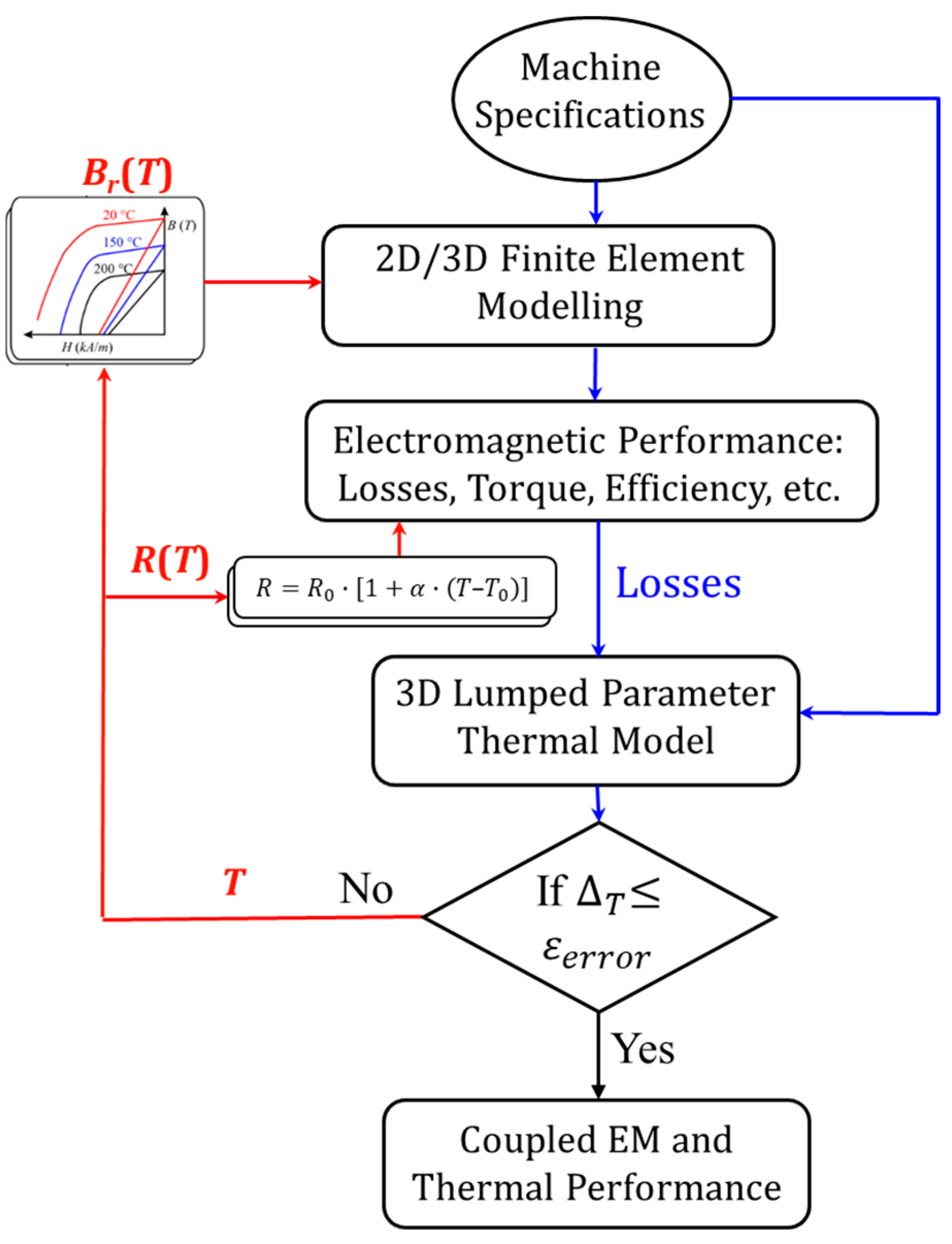
Although several prior works have already been conducted to show the superior electromagnetic (EM) performances of modular machines, little research has been aimed at the coupled EM–thermal modelling of their dynamic performances [13]. For variable speed high torque/power density application, the coupled EM–thermal modelling is particularly important for accurately predicting machine dynamic performance under different operating conditions. This is mainly because when machine temperature increases, magnet remanent flux density reduces, leading to reduced magnetic loading and hence reduced output torque/power [7,14]. To maintain the same level of output torque, the phase current (electrical loading) often needs to be increased to compensate the reduced magnetic loading. Together with the increased copper resistivity due to temperature rise, the copper loss can be significantly increased [15]. This might lead to reduced machine efficiency. In addition, as a main heat source, the increased copper loss will lead to further temperature rise and also further reduced magnet remanent flux density [16,17]. Without coupled EM–thermal modelling, this mutual effect between thermal performance and EM performance cannot be accurately predicted. Therefore, to reveal the full potential of the modular machines, the coupled EM–thermal models are proposed in this paper to investigate their steady-state dynamic performances and compare against the conventional non-modular machines. The steady-state EM performances at different speed for investigated machines have been studied. The flowchart depicting the coupled EM–thermal analysis is shown in Figure 2. The machine specifications shown in Table 1 and also the initial temperature are used to calculate the initial EM performance, such as the torque and losses. The losses are then adopted as the input in the 3D lumped parameter thermal network for the thermal analysis. The obtained temperature can be used for updating the magnet properties [based on the temperature-dependent B(H) curves] and coil resistance for each iteration. When the temperature difference ( Δ T ) is lower than the convergence error ( ε e r r o r ), the final temperature distribution and EM performance can be obtained.

2. Dynamic Performance Analysis

The steady-state dynamic performances, such as torque speed curve and efficiency map, are critical for variable speed applications, such as electrical vehicles, more electrical aircraft, and so on. However, in the literature, many papers focus on the dynamic performance without considering the EM–thermal coupling. This might not be able to predict the real dynamic performance as the temperature rise within electrical machines has significant impact on magnet demagnetization, phase resistance, etc. For the same phase current, the temperature rise could lead to increased copper loss, reduced average torque, reduced stator, and rotor core iron losses, and hence have a significant impact on machine dynamic performance, such as torque speed curve and efficiency map. In this paper, the modelling with and without considering the EM–thermal coupling is carried out for the modular SPM machines to reveal the influence of temperature rise on their dynamic performance.

2.1. Without EM–Thermal Coupling

For comparison purposes, the torque speed curve and efficiency map for both the modular and non-modular machines are investigated in this section without considering the EM–thermal coupling.

2.1.1. Torque Speed Curve

The EM behavior of PM machines is governed by the stator voltage equations. In a synchronous reference frame, they can be written as,
V d = R i d + L d d i d d t ω e L q i q
V q = R i q + L q d i q d t + ω e L d i d + ψ m ω e
where V , i , ω e , L , R , ψ m denote the voltage, current, rotor electrical speed, inductance, resistance, and no-load flux linkage, respectively. The subscripts d and q represent the direct- and quadrature-axis components.
The EM torque ( T e m ) and output power ( P o u t ) can be derived as:
T e m = 3 2 p [ ψ m i q + ( L d L q ) i d i q ]
P o u t = T e m ω m
where ω m = ω e /p is the rotor mechanical speed.
If the rated phase current ( i s ) and the DC-link voltage ( 3 V s ) for a standard space vector pulse width modulation (SVPWM) control are given, the torque speed curve of PM machines can be calculated using equations from (1) to (3). Furthermore, if the phase resistance is neglected, the base-speed ( ω b ) and the maximum speed ( ω m a x ) can be calculated by
ω b = V s ( p ψ m 2 + ( L q i s ) 2 )
ω m a x = V s [ p ( ψ m L d i s ) ]
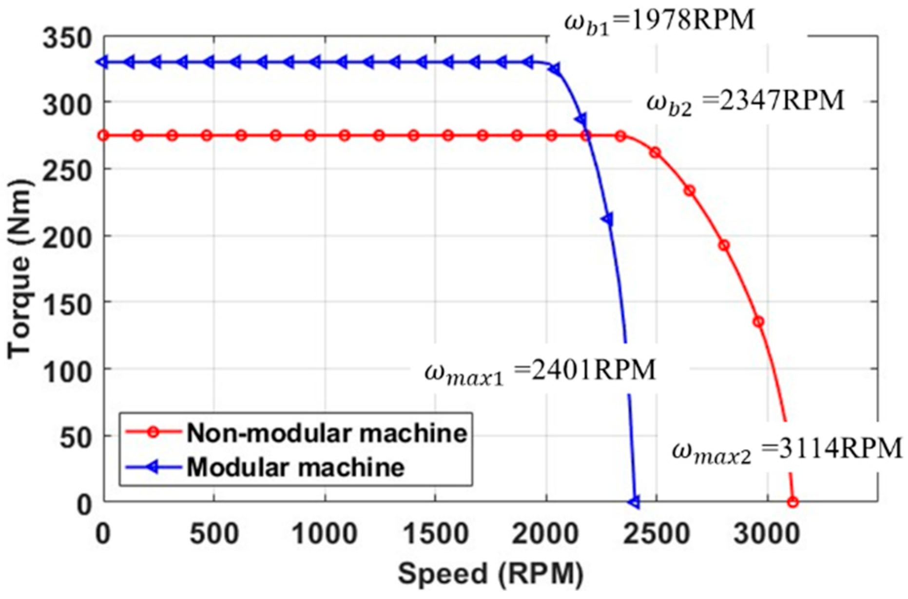
The torque speed curves for the investigated machines are shown in Figure 3. It is worth noting that when the rotor speed is lower than the base-speed, the machine is operated at constant torque region (maximum torque per ampere). When the rotor speed is beyond the base-speed, the machine enters the flux weakening region, and the d-axis current is increased with the increased rotor speed. It is found that compared with the conventional non-modular SPM machine, the modular SPM machine has better performance in the constant torque region due to higher ψ m , which is achieved by adopting a suitable flux gap width. However, the increased ψ m reduces the base speed and also the maximum speed for the modular machine as can be concluded from (5) and (6). Therefore, the high-speed performance during the flux weakening operation of the modular SPM machine is worsened.

2.1.2. Losses Speed Curve

In this paper, the EM performance is simulated by 2D FEM. This is accurate enough for calculating performances, such as flux linkage, phase back-EMF, on-load torque, and stator and rotor core iron losses. However, during the calculation of PM eddy current losses, the axial and circumferential eddy currents at the PM end region are excluded from the calculation of 2D FEM. Therefore, in order to have precise PM eddy current loss results, a 3D/2D correction factor ( F ) is introduced as [18]
F = 3 4 · L 2 w 2 + L 2
where the L and w denote the PM axial length and width, respectively.
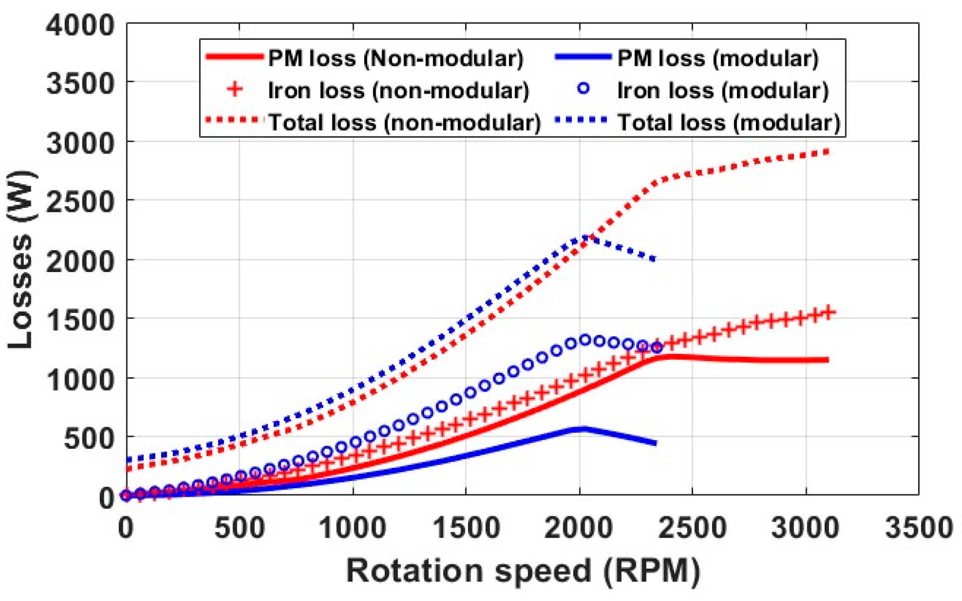
The stator and rotor core iron losses as well as PM eddy current loss against speed have also been calculated, as shown in Figure 4. It is found that in the constant torque region, the losses, including the PM eddy current losses and stator and rotor iron losses, will all increase with rotor speed for both the investigated machines. In addition, compared with the non-modular machine, the modular machine has lower PM eddy current loss but higher stator and rotor core iron losses. This is mainly due to the introduced flux gaps that lead to increased fundamental and reduced harmonic components in the airgap flux density. Together with the higher copper loss caused by the reduced slot area, the total loss of the modular machine is slightly higher than that of the non-modular machine at the constant torque region. However, in the flux weakening region, the increase rates of both the stator and rotor core iron losses as well as the PM eddy current loss of the non-modular machine have been reduced due to the demagnetization caused by the increase in d-axis current. For the modular machine, its stator and rotor core iron losses as well as the PM eddy current loss even reduce. Beyond 2300 rpm, the iron loss of the modular machine can be even lower than that of the non-modular machine.

2.1.3. Efficiency Map

Using the previously calculated iron losses ( P i ) and the PM eddy current loss ( P m ) together with the copper loss ( P c ), the efficiency ( η ) can be calculated by
η = P o u t P o u t + P i + P m + P c
The efficiency maps for the modular and non-modular machines are shown in Figure 5. It is worth noting that in this figure the efficiency below 60% has been neglected. It can be found that compared with the non-modular machine, the modular machine has a wider high-efficiency range. Even the total loss of the modular machine is slightly higher than that of the non-modular machine; a significant improvement in torque at the constant torque region results in slightly higher efficiency under most operation conditions.

2.2. With EM–Thermal Coupling

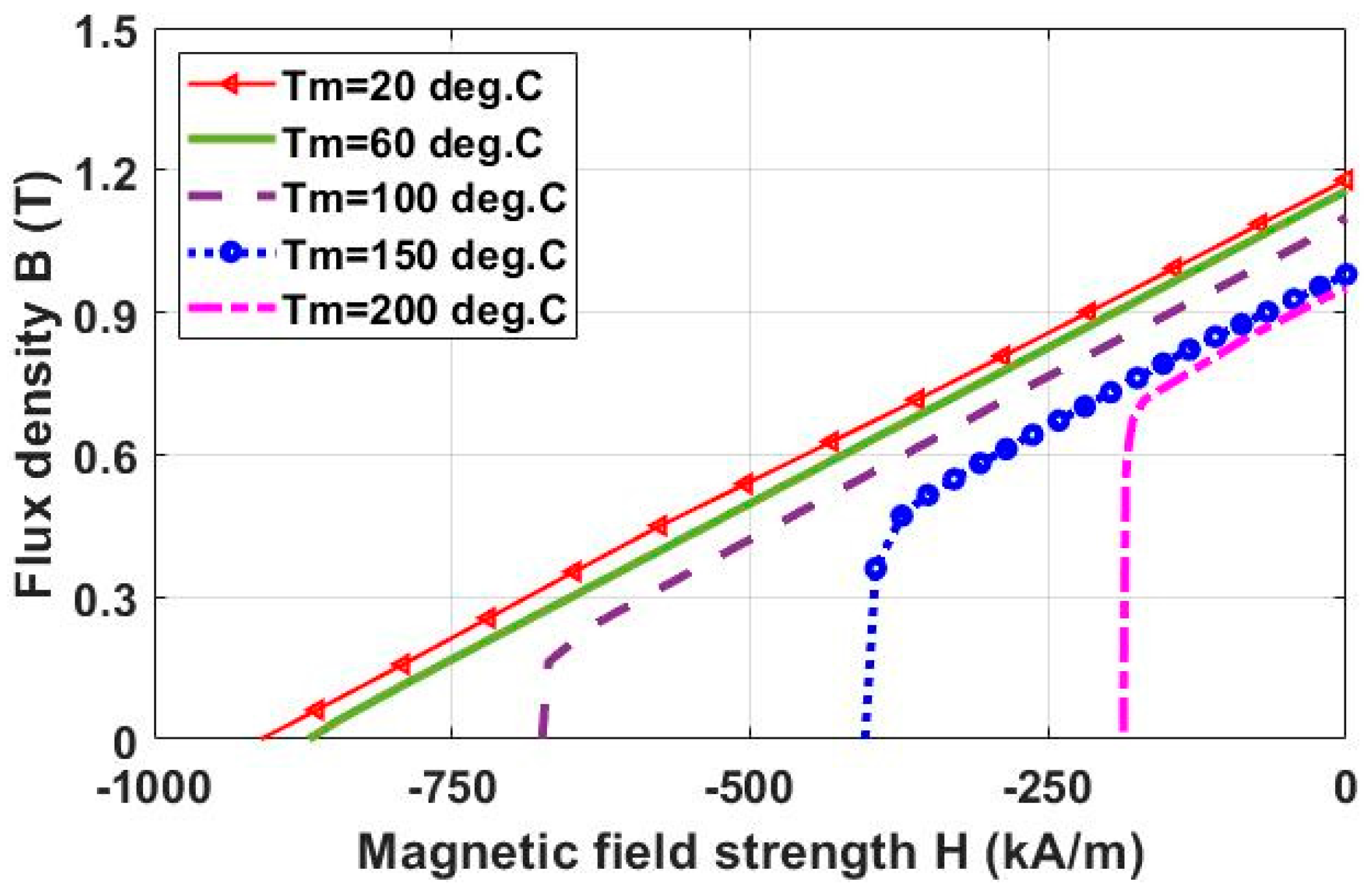
As mentioned previously, the above analyses do not consider the EM–thermal coupling. However, the temperature rise has a significant impact on the temperature-dependent magnet B(H) curve and copper resistivity; hence it will also have significant influence on the dynamic performance. For the magnet material used in this paper, its B(H) curves at different operating temperatures are shown in Figure 6. The remanence ( B r ) and coercivity ( H c ) are both reduced with temperature rise, and the temperature-dependent B r and H c can be written as [14]
{ B r ( T ) = B r ( T 0 )   [ 1 + α 1 ( T T 0 ) + α 2 ( T T 0 ) 2 ] H c ( T ) = H c ( T 0 )   [ 1 + β 1 ( T T 0 ) + β 2 ( T T 0 ) 2 ]
where T 0 is the reference temperature, and α 1 , α 2 , β 1 , and β 2 are temperature-dependent coefficients. In practice, it is often found that α 1 α 2 and β 1 β 2 . For example, for the magnet used in this paper, α 1 = 1.2 × 10 3 , α 2 = 1.5 × 10 9 , β 1 = 6.9 × 10 3 , and β 2 = 1.17 × 10 5 .

2.2.1. Temperature-Dependent PM Flux Linkage and Inductance

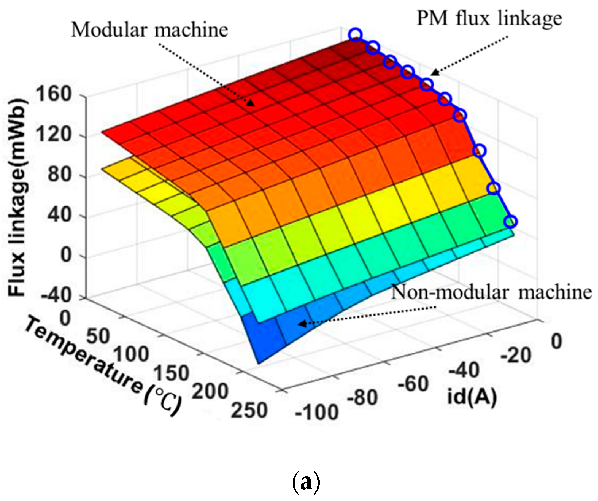
Considering the temperature-dependent properties of the magnets shown in Figure 6, the flux linkage, d- and q-axis inductances have been calculated by 2D FEM, as shown in Figure 7. These parameters will be used for calculating the temperature-dependent dynamic performance of the modular and non-modular machines. It is shown in Figure 7a that the d-axis flux linkage of the modular machine is always higher than that of the non-modular machine regardless of the operating conditions. This means that for a constant q-axis current, the torque of the modular machine will always be higher than that of the non-modular machine as described by (3). In addition, when the magnet temperature is larger than 150   ° C , there is a significant reduction in the PM flux linkage for both the investigated machines due to magnet irreversible demagnetization.
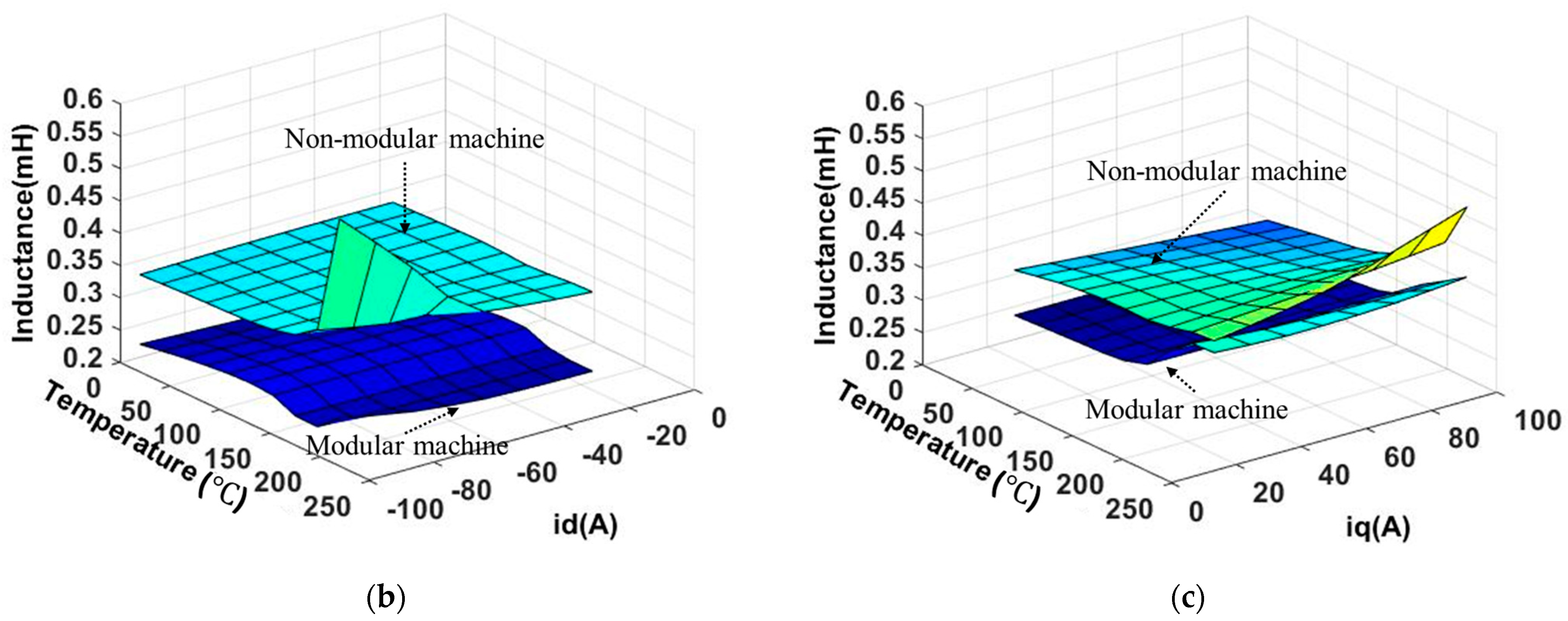
Apart from the PM flux linkage, the d- and q-axis inductances vary with magnet temperature and current as well, which can also affect the dynamic performances as described by the equations from (3) to (6). As shown in Figure 7b,c, due to the existence of flux gaps, the d- and q-axis inductances of the modular machine are generally smaller than those of the non-modular machine for different currents and operating temperatures. In addition, the inductances for both the investigated machines increase with temperature rise. This is because at higher temperature, the magnet remanence Br reduces, and so does the saturation level. This leads to a reduced effective airgap length and hence increased d- and q-axis inductances.
When temperature rises, the copper loss is also increased, which can be determined by using the temperature-dependent coefficient ( 3.69 × 10 3 /   ° C ) of the electrical resistivity for copper. Here, the reference temperature is 20 °C [15]. This increase in copper loss needs to be feedback to the thermal modelling as it is one of the main heat sources. Therefore, a closed-loop coupling between EM and thermal modelling needs to be implemented as described by the flowchart shown in Figure 2 for dynamic performance analysis. Some assumptions need to be made for the closed-loop coupling analysis, such as:
(a)
The electrical resistivity of the PM and iron core are independent of temperature variation. This is safe as when temperature increases within a limited range, the increase in resistivity of the PM and iron core can be largely negligible [19].
(b)
The investigated machines are designed for the direction control of helicopters that do not require continuous operation. Hence, the duty ratio of 0.2 for the investigated machines has been adopted, and one cycle lasts for 4000 s.
(c)
The allowable convergence error ( ε e r r o r ) is set to be 0.5% in this paper.
It is worth noting that the convergence error ( Δ T ) is identified as the magnet temperature difference described by
Δ T = T n T n 1 T n 1

2.2.2. Temperature Speed Curve

In the coupled EM–thermal models for dynamic performance analysis, the temperature variation is critical as it has a direct impact on the PM remanent flux density, coercivity, and phase resistance. To accurately predict the temperature variation for different operating conditions, the Lumped Parameter Thermal Network (LPTN) will be adopted. The LPTN modelling is a well-documented method which is accurate and less time-consuming compared to finite element (FE) modelling and computational fluid dynamic (CFD) modelling. These are very desirable features for the coupled EM–thermal modelling in this paper as temperature distributions under numerous operating conditions are required for the dynamic performance analysis. It is worth noting that the steady-state LPTN modelling will be used for the thermal analysis in this paper because only the maximum magnet temperature is required to evaluate the most significant magnet demagnetization. It means that during the FE modelling for EM analysis, the PM temperature is assumed to be uniform, and the value is obtained from LPTN. There are two important components in the steady-state LPTN models. One is the heat source, and the other is the thermal resistances. The losses (heat sources in the LPTN model) for the investigated machines have been calculated previously in Section 2.1.2. The equivalent thermal resistances due to conduction ( R t h ), convection ( R h ), and radiation ( R r ) can be calculated by
{ R t h = L λ S t h R h = 1 h S h R r = 1 α t h S h
where L and S t h are the length of the heat path and the cross-sectional area for conductive heat transfer, respectively. S h is the heat transfer area by convection and radiation, while λ , h , and α t h are thermal conductivity, convection, and radiation coefficients, respectively. It is worth noting that the equation of conduction is only for a bar without heat generation in it. However, when the bar has heat generated in it, a modified equivalent thermal resistance ( R t h = L 4 λ S t h ) is necessary to obtain a more accurate machine temperature prediction. To simplify the calculations, some components (such as rotor, stator back iron, housing, and shaft) are considered as cylindrical components. Others (such as PMs, coil active windings, and end-windings) are considered as cylindrical components with angular spans. Their equivalent thermal resistances are more complicated. Details about the calculations of thermal resistances of different components within electrical machines can be found in the Appendix A.
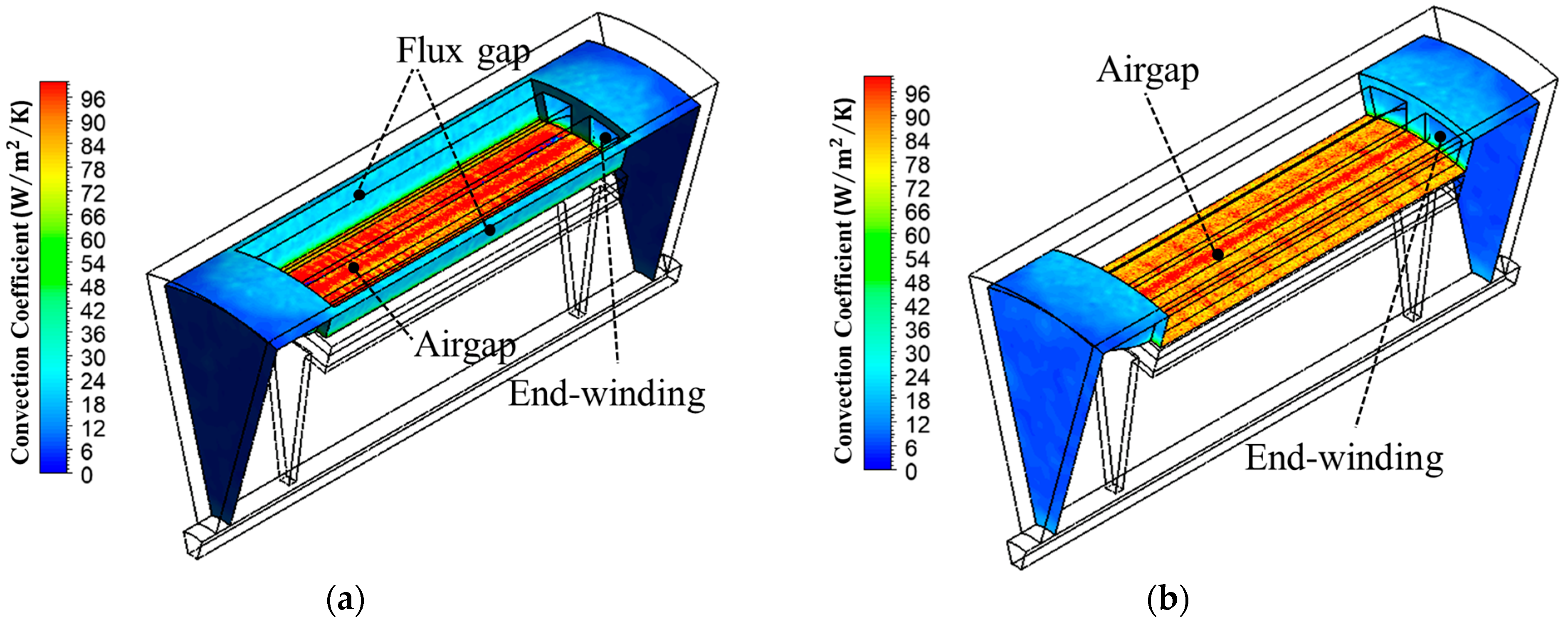
In the LPTN model, the thermal conductivities of different materials are generally known. However, the convection coefficients on different surfaces are difficult to obtain. This is particularly the case for surfaces in the airgap, in flux gaps, on end-windings, etc. To calculate these thermal convection coefficients, 3D CFD modelling has been adopted. By way of example, the results at the rated speed (1500 rpm) for modular and non-modular machines are shown in Figure 8. It is worth noting that both the modular and non-modular machines are totally enclosed without fan cooling, and their convection coefficients on different surfaces are largely similar. However, the introduced flux gaps can increase the contact surface area and reduce the equivalent thermal resistance as described by (11). As a result, they have the potential to improve machine internal cooling.
It is worth noting that the convection coefficient distribution shown in Figure 8 is estimated by the direct approach as [20]
h i = q i ( T w i T a i ) A i
where h i , q i , A i , and T w i are the convection coefficient, heat flux, heat exchange surface area, and temperature of the target mesh element, respectively. T a i is the temperature of air that is adjacent to the target mesh element which may not be the same for different meshes. Therefore, the convection coefficient calculated by this direct approach is not accurate enough for the LPTN modelling. In order to adapt to the LPTN, the average convection coefficient ( h ¯ ) on different surfaces should be re-written by
h ¯ = ( A i q i ) ( A i T wi ) T a A i
where T a is the average temperature of air within the investigated machines. According to (13), the equivalent thermal resistances that represent the thermal convection are derived by
R c = 1 h ¯ · A i
A modified convection coefficient and equivalent thermal resistance are more suitable for establishing the LPTN model. For the LPTN built in this paper, all equivalent thermal resistances that represent components inside the machine are linked to only one node, i.e., the node that represents the air inside the machine. Therefore, employing the average temperature of air obtained from CFD modeling as a reference temperature for calculating the convection coefficient can achieve an accurate temperature prediction.
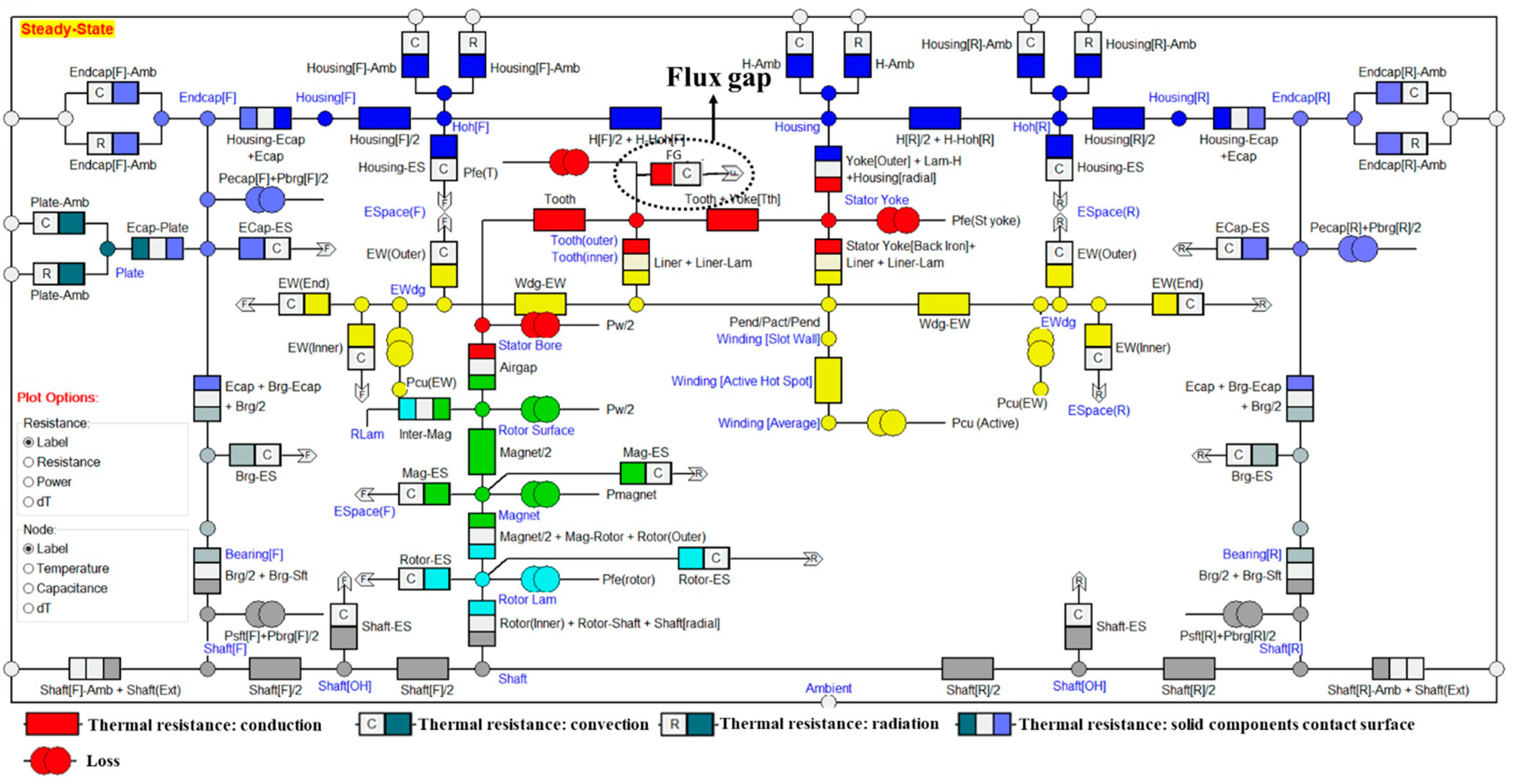
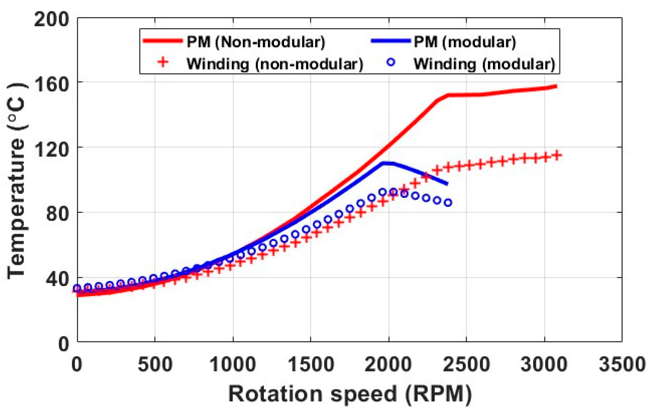
The simplified LPTN for the modular machine is developed based on the model in Motor-CAD v13.1 as shown in Figure A3 (see Appendix A). It is worth noting that the heat convection from the flux gap surfaces to air should be introduced to obtain more accurate machine temperature distribution for the modular machines. The equivalent thermal resistances can be calculated by (A1) to (A13). The steady-state temperatures of PMs at different rotor speeds have been calculated by the LPTN as shown in Figure 9. Like the trend of losses presented in the previous section, the temperatures within both machines increase with increasing rotor speed. It is also found that when the rotor speed is low, the magnet temperatures within the modular machine are slightly higher than those within the non-modular machine due to higher copper loss and iron losses. However, when the rotor speed is beyond the base speed, the temperatures within the modular machine are reduced due to the influence of magnet demagnetization. In addition, to prevent the PM from irreversible demagnetization, the critical temperature of the PM material chosen in this paper is around 150 °C [21]. It can be seen that the magnet temperature in the modular machine is always lower than the critical temperature for the full speed range. By contrast, the temperature of the non-modular machine can go beyond the critical temperature, leading to potentially serious irreversible demagnetization.

2.2.3. Dynamic Performance

To evaluate the impact of temperature rise on machine EM performance, the temperature-dependent B(H) curve and the temperature speed curve are implemented to re-evaluate the torque speed curve for the modular and non-modular machines, as shown in Figure 10. It is worth noting that the EM performances of the machines without the coupled model do not consider the influence of temperature variation within the machine. The material properties are all chosen at 20 °C. In contrast, the EM performances obtained by the coupled model fully consider the thermal influence. This includes the impact of temperature on PM demagnetization and copper resistance. It can be found that for both machines, when the demagnetization caused by temperature rise is considered, the torque is reduced due to reduced PM flux-linkage. Furthermore, the increased temperature improves both the base and maximum speeds, also due to reduced PM flux-linkage as calculated by (5) and (6). Therefore, although the demagnetization can reduce the EM performance in the constant torque region, it can improve the performance in the flux weakening region.
As shown in Figure 11, the iron losses and PM eddy current losses are reduced due to the demagnetization caused by temperature rise. It is worth noting that the losses at each speed have been calculated under the condition that the investigated machines operate under maximum torque per ampere or per volt control. However, the copper loss will be increased due to the increase in coil temperature. These variations in losses and also on-load torque due to temperature rise will lead to a significant change in the efficiency maps for the modular and non-modular machines, as shown in Figure 12. It can also be found that, similar to the EM-only predictions, although both machines have similar peak efficiency, the area for peak efficiency of the modular machine is larger than that of the non-modular machine.

3. Conclusions

In this paper, the dynamic performance considering the EM–thermal coupling has been investigated for both the modular and non-modular machines. Compared to the non-coupled EM-only analysis, the coupled EM–thermal modelling can consider the effect of temperature rise on magnet properties, e.g., the remanence and coercivity and copper resistivity. For example, at a given temperature, the EM performance, such as the PM flux linkage, stator and rotor core iron losses, PM eddy current loss, and copper loss, can be calculated. The calculated losses will be used as input in the thermal model to calculate an updated temperature distribution, which, in turn, will allow the calculation of updated EM performance. This will make accurate analysis of dynamic performance under different operating conditions possible. Based on the results obtained by the coupled EM–thermal models, it was found that compared with the non-modular machine, the modular machine generally has higher torque and efficiency under different operating conditions. This is mainly due to the introduced flux gaps in alternate stator teeth that can be used to boost both the EM and thermal performances. The flux gaps result in high torque density and better demagnetization withstand capability. In addition, the flux gaps also provide additional cooling channels that can reduce the machine temperature, especially the PM temperature. In conclusion, the performance improvements of the modular machine have been fully revealed according to the coupled EM–thermal modelling of steady-state dynamic performances.

Author Contributions

Writing—original draft, W.Z.; writing—review and editing, G.-J.L. and Z.-Q.Z.; funding acquisition, B.R. and Y.C.C. All authors have read and agreed to the published version of the manuscript.

Funding

This work is partially supported by the UK Engineering and Physical Science Research Council (EPSRC) under Grant No. EP/T017988/1 and partially sponsored by Motor Design Ltd., An Ansys Company.

Data Availability Statement

Not applicable.

Acknowledgments

We would like to thank Melanie Michon (Motor Design Ltd., now ANSYS) for providing the financial support for this work.

Conflicts of Interest

The authors declare no conflict of interest.

Appendix A

In the thermal analysis using LPTN model, electrical machines can be divided into serval hollow cylinders, which is the case for the rotor and stator yokes, as shown in Figure A1a. However, the magnets, coils, stator teeth and end-windings can be regarded as cylindrical components with different angular spans, as shown in Figure A1b.
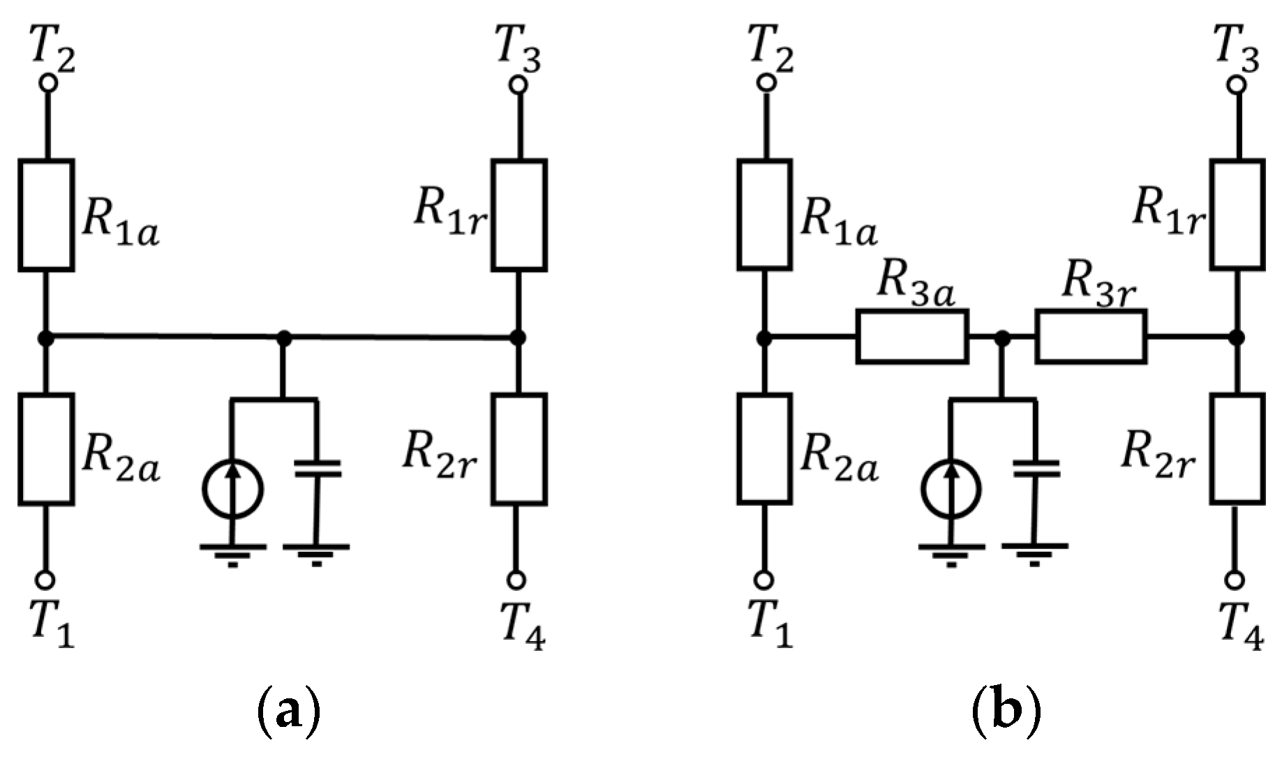
For the components without heat generation, e.g., shaft and housing, their heat transfer can be represented by the equivalent LPTN shown in Figure A2a. Their equivalent resistances are derived by [22,23,24,25]
R 1 r = 1 4 π λ L [ 1 2 r 2 2 ln ( r 1 r 2 ) ( r 1 2 r 2 2 ) ]
R 2 r = 1 4 π λ L [ 2 r 1 2 ln ( r 1 r 2 ) ( r 1 2 r 2 2 ) 1 ]
R 1 a = R 2 a = L 2 π λ ( r 1 2 r 2 2 )
Figure A1. Cylindrical components in electrical machines. (a) Whole component and (b) with angular spans α . r 1 , r 2 and L are the radius of inner surface, radius of outer surface and stack length, respectively. T 1 , T 2 , T 3 and T 4 are the temperatures of the front, rear, outer and inner surfaces.
Energies 16 02516 g0a1
Figure A2. Equivalent LPTN for cylindrical components. (a) Without and (b) with heat generation.
Energies 16 02516 g0a2
However, for components with heat generated inside them such as the stator and rotor iron cores and magnets, a third equivalent thermal resistance R3 needs to be introduced, as shown in Figure A2b. The values of R3 in radial and axial directions have been derived using
R 3 r = 1 8 π λ L ( r 1 2 r 2 2 ) [ ( r 1 2 + r 2 2 ) 4 r 2 2 ln ( r 1 r 2 ) ( r 1 2 r 2 2 ) ]
R 3 a = L 6 π λ ( r 1 2 r 2 2 )
Similarly, for the coils, teeth and end-windings having different angular spans α , their equivalent thermal resistances can be derived by [26]
R 1 r = 1   2 α λ L [ 1 2 r 2 2 ln ( r 1 r 2 ) ( r 1 2 r 2 2 ) ]
R 2 r = 1   2 α λ L [ 2 r 1 2 ln ( r 1 r 2 ) ( r 1 2 r 2 2 ) 1 ]
R 1 a = R 2 a = L α λ ( r 1 2 r 2 2 )
R 3 r = 1 4 α λ L ( r 1 2 r 2 2 ) [ ( r 1 2 + r 2 2 ) 4 r 2 2 ln ( r 1 r 2 ) ( r 1 2 r 2 2 ) ]
R 3 a = L 3 α λ ( r 1 2 r 2 2 )
The consideration of heat transfer in circumferential direction for coils and teeth is also necessary. They can be regarded as trapezoidal components, and their equivalent thermal resistances can be derived by [27]
R 1 c = R 2 c = α λ L ln ( r 1 r 2 )
R 3 c = α 3 λ L ln ( r 1 r 2 )
The coil with insulation and potting compound has been regarded as an ideal material with anisotropic thermal conductivity. By assuming that the thermal properties of the insulation layer is close to the potting compound, the Hashin and Shtrikman approximation is able to estimate the equivalent thermal conductivity ( λ e ) in the direction which is perpendicular to the direction of current as [28]
λ e = λ p ( 1 + ν c ) λ c + ( 1 ν c ) λ p ( 1 ν c ) λ c + ( 1 + ν c ) λ p
where the copper volume ratio ν c is taken to be equal to the packing factor. The subscripts c and p represent the conductors and impregnation, respectively.
The LPTN model of the non-modular machine can be developed using Motor-CAD software package. This is the same for the modular machine. The difference however is that, due to the existence of the flux gaps, extra thermal resistances due to convection will be needed in the LPTN model of the modular machine, as shown in Figure A3. As mentioned previously, the convection coefficients have been calculated using 3D CFD modelling, as shown in Figure 8.
Figure A3. LPTN model based on Motor-CAD for the modular machine.
Energies 16 02516 g0a3

References

  1. Gerada, C.; Galea, M.; Kladas, A. Electrical Machines for Aerospace Applications. In Proceedings of the 2015 IEEE Workshop on Electrical Machines Design, Control and Diagnosis (WEMDCD), Torino, Italy, 26–27 March 2015; pp. 79–84. [Google Scholar]
  2. Galea, M.; Xu, Z.; Tighe, C.; Hamiti, T.; Gerada, C.; Pickering, S. Development of an Aircraft Wheel Actuator for Green Taxiing. In Proceedings of the 2014 International Conference on Electrical Machines (ICEM), Berlin, Germany, 2–5 September 2014; pp. 2492–2498. [Google Scholar]
  3. Ishak, D.; Zhu, Z.Q.; Howe, D. Permanent Magnet Brushless Machines with Unequal Tooth Widths and Similar Slot and Pole Numbers. In Proceedings of the 2004 IEEE Industry Applications Conference, 39th IAS Annual Meeting, Seattle, WA, USA, 3–7 October 2004; pp. 1055–1061. [Google Scholar]
  4. Tapia, J.A.; Leonardi, F.; Lipo, T.A. Consequent-pole permanent-magnet machine with extended field-weakening capability. IEEE Trans. Ind. Appl. 2003, 39, 1704–1709. [Google Scholar] [CrossRef] [Green Version]
  5. Li, G.; Zhu, Z. Analytical modeling of modular and unequal tooth width surface-mounted permanent magnet machines. IEEE Trans. Magn. 2015, 51, 1–9. [Google Scholar] [CrossRef] [Green Version]
  6. Li, G.; Ren, B.; Zhu, Z.; Foster, M.; Stone, D. Demagnetization withstand capability enhancement of surface mounted PM machines using stator modularity. IEEE Trans. Ind. Appl. 2017, 54, 1302–1311. [Google Scholar] [CrossRef] [Green Version]
  7. Zhang, W.; Li, G.J.; Zhu, Z.Q.; Ren, B.; Chong, Y.C.; Michon, M. Demagnetization Analysis of Modular SPM Machine Based on Coupled Electromagnetic–Thermal Modelling. Energies 2022, 16, 131. [Google Scholar] [CrossRef]
  8. Li, G.J.; Liang, X.B.; Zhu, Z.Q.; Ojeda, J.; Gabsi, M. Vibrations and Acoustic Noise Analyses of Modular SPM Machines. In Proceedings of the 2020 IEEE Energy Conversion Congress and Exposition (ECCE), Detroit, MI, USA, 11–15 October 2020; pp. 5567–5573. [Google Scholar]
  9. Zhou, R.; Li, G.J.; Zhang, K.; Zhu, Z.; Foster, M.; Stone, D. Performance Investigation of Consequent-Pole PM Machines with E-core and C-core Modular Stators. IEEE Trans. Energy Convers. 2020, 36, 1169–1179. [Google Scholar] [CrossRef]
  10. Taras, P.; Li, G.J.; Zhu, Z.Q. Comparative study of fault-tolerant switched-flux permanent-magnet machines. IEEE Trans. Ind. Electron. 2016, 64, 1939–1948. [Google Scholar] [CrossRef]
  11. Chen, Z.; Spooner, E. A modular, permanent-magnet generator for variable speed wind turbines. In Proceedings of the Seventh International Conference on Electrical Machines and Drives, Durham, UK, 11–13 September 1995; pp. 453–457. [Google Scholar]
  12. Zhang, W.; Li, G.J.; Zhu, Z.Q.; Ren, B.; Michon, M. Optimization of Modular SPM Machines Considering Stator Modularity. In Proceedings of the International Electric Machines and Drives Conference (IEMDC), Hartford, CT, USA, 17–20 May 2021. [Google Scholar]
  13. Joo, D.; Cho, J.H.; Woo, K.; Kim, B.-T.; Kim, D.K. Electromagnetic field and thermal linked analysis of interior permanent-magnet synchronous motor for agricultural electric vehicle. IEEE Trans. Magn. 2011, 47, 4242–4245. [Google Scholar] [CrossRef]
  14. Zhou, P.; Lin, D.; Xiao, Y.; Lambert, N.; Rahman, M. Temperature-dependent demagnetization model of permanent magnets for finite element analysis. IEEE Trans. Magn. 2012, 48, 1031–1034. [Google Scholar] [CrossRef]
  15. Dellinger, J.H. The Temperature Coefficient of Resistance of Copper; US Government Printing Office: Washington, DC, USA, 1911. [Google Scholar]
  16. Jiang, W.; Jahns, T.M. Development of Efficient Electromagnetic-Thermal Coupled Model of Electric Machines Based on Finite Element Analysis. In Proceedings of the 2013 International Electric Machines & Drives Conference, Chicago, IL, USA, 12–15 May 2013; pp. 816–823. [Google Scholar]
  17. Shi, Y.; Wang, J.; Wang, B. Electromagnetic-thermal coupled simulation under various fault conditions of a triple redundant 9-phase PMASynRM. IEEE Trans. Ind. Appl. 2019, 56, 128–137. [Google Scholar] [CrossRef]
  18. Ruoho, S.; Santa-Nokki, T.; Kolehmainen, J.; Arkkio, A. Modeling magnet length in 2-D finite-element analysis of electric machines. IEEE Trans. Magn. 2009, 45, 3114–3120. [Google Scholar] [CrossRef]
  19. Wu, K.; Yao, Y.; Klik, I. Electrical and magnetic properties of NdFeB films. Appl. Surf. Sci. 1997, 113, 174–177. [Google Scholar] [CrossRef]
  20. Micallef, C. End Winding Cooling in Electric Machines; University of Nottingham: Nottingham, UK, 2006. [Google Scholar]
  21. Sebastian, T. Temperature effects on torque production and efficiency of PM motors using NdFeB magnets. IEEE Trans. Ind. Appl. 1995, 31, 353–357. [Google Scholar] [CrossRef]
  22. Nerg, J.; Rilla, M.; Pyrhonen, J. Thermal analysis of radial-flux electrical machines with a high power density. IEEE Trans. Ind. Electron. 2008, 55, 3543–3554. [Google Scholar] [CrossRef]
  23. Gerling, D.; Dajaku, G. Novel Lumped-Parameter Thermal Model for Electrical Systems. In Proceedings of the 2005 European Conference on Power Electronics and Applications, Dresden, Germany, 11–14 September 2005; p. 10. [Google Scholar]
  24. El-Refaie, A.M.; Harris, N.C.; Jahns, T.M.; Rahman, K.M. Thermal analysis of multibarrier interior PM synchronous machine using lumped parameter model. IEEE Trans. Energy Convers. 2004, 19, 303–309. [Google Scholar] [CrossRef] [Green Version]
  25. Roberts, D. The Application of an Induction Motor Thermal Model to Motor Protection and Other Functions. Ph.D. Thesis, University of Liverpool, Liverpool, UK, 1989. [Google Scholar]
  26. Mezani, S.; Takorabet, N.; Laporte, B. A combined electromagnetic and thermal analysis of induction motors. IEEE Trans. Magn. 2005, 41, 1572–1575. [Google Scholar] [CrossRef]
  27. Liu, Z.; Howe, D.; Mellor, P.; Jenkins, M. Thermal Analysis of Permanent Magnet Machines. In Proceedings of the 1993 Sixth International Conference on Electrical Machines and Drives (Conf. Publ. No. 376), Oxford, UK, 8–10 September 1993; pp. 359–364. [Google Scholar]
  28. Simpson, N.; Wrobel, R.; Mellor, P.H. Estimation of equivalent thermal parameters of impregnated electrical windings. IEEE Trans. Ind. Appl. 2013, 49, 2505–2515. [Google Scholar] [CrossRef]
Figure 1. Cross sections and open-circuit flux line distribution of SPM machines: (a) modular machine; (b) non-modular machine.
Energies 16 02516 g001
Figure 2. Flowchart of the coupled EM–thermal modelling. T, B r , R , and ε e r r o r are the temperature, magnet remanence, phase resistance, and convergence error, respectively.
Energies 16 02516 g002
Figure 3. Torque-speed curves for the modular and non-modular machines at room temperature (20 °C) without considering EM–thermal coupling.
Energies 16 02516 g003
Figure 4. Losses-speed curves for the modular and non-modular machines operating at room temperature (20 °C).
Energies 16 02516 g004
Figure 5. Efficiency maps at room temperature (20 °C) without considering EM–thermal coupling: (a) modular machine; (b) non-modular machine.
Energies 16 02516 g005
Figure 6. Temperature-dependent B(H) curves for PM material used in this paper.
Energies 16 02516 g006
Figure 7. (a) The d-axis flux linkage; (b) d-axis inductance; (c) q-axis inductance vs. d- or q-axis axis current and magnet temperature for both the modular and non-modular machines.
Energies 16 02516 g007aEnergies 16 02516 g007b
Figure 8. Convection coefficient distribution on different surfaces inside (a) a modular machine and (b) a non-modular machine. The rotor speed is 1500 rpm.
Energies 16 02516 g008
Figure 9. Magnet and winding temperature speed curves of modular and non-modular machines.
Energies 16 02516 g009
Figure 10. Torque speed curves of (a) the modular machine and (b) the non-modular machine with or without considering the EM–thermal coupling.
Energies 16 02516 g010
Figure 11. Losses speed curve of (a) the modular machine and (b) the non-modular machine with and without the EM–thermal coupling.
Energies 16 02516 g011
Figure 12. Efficiency maps of (a) the modular machine and (b) the non-modular machine considering the EM–thermal coupling.
Energies 16 02516 g012
Table 1. Parameters of modular SPM machine.
Slot number24Rotor outer radius (mm)129.4
Pole number28Rotor yoke thickness (mm)8.6
Stator outer radius (mm)154Stack length (mm)210
Stator yoke height (mm)5.6DC voltage (V)800
Tooth width (mm)13.2Rated phase current ( A p e a k )100
Flux gap width (mm)10Number of turns per coil 10
Airgap length (mm)2Rate speed (rpm)1500
Magnet thickness (mm)6.6
Disclaimer/Publisher’s Note: The statements, opinions and data contained in all publications are solely those of the individual author(s) and contributor(s) and not of MDPI and/or the editor(s). MDPI and/or the editor(s) disclaim responsibility for any injury to people or property resulting from any ideas, methods, instructions or products referred to in the content.