Probabilistic Power Flow Method for Hybrid AC/DC Grids Considering Correlation among Uncertainty Variables

Abstract

For a new power system using high-penetration renewable energy, the traditional deterministic power flow analysis method cannot accurately represent the stochastic characteristics of each state variable. The aggregation of renewable energy with different meteorological characteristics in the AC/DC interconnected grid significantly increases the difficulty of establishing a steady-state model. Therefore, this study proposes an improved Latin hypercube sampling algorithm using the van der Waerden scores and diffusion kernel density estimation to overcome the limitations of a priori assumption on probability distributions in uncertainty modeling and to retain the correlations among random variables in the sampling data. Interconnected grids are constructed with IEEE 9-bus and IEEE 14-bus and modified with IEEE 57-bus to describe common application cases of aggregated renewable energy. On this basis, the approximation errors of the proposed probabilistic power flow algorithm to the statistical characteristics of the power parameters are evaluated by setting the Nataf algorithm and the Latin hypercube algorithm using adaptive kernel density estimation as the control group. The results show that the improved Latin hypercube sampling algorithm can exhibit high computational accuracy and strong adaptability, both in severe operating scenarios with large amplitude of load fluctuations and with nonlinear power balance equations incorporating high dimensional random variables.

1. Introduction

The continuous and excessive exploitation and utilization of fossil fuels have led to the global greenhouse effect, which has become a significant barrier to economic and social development. In response, countries highly value renewable energy sources (REs), such as wind and solar energy, due to their inexhaustible resource attributes and zero-emission characteristics in power generation. Therefore, promoting the development of renewable energy is crucial to achieving carbon neutrality [1,2]. However, as the permeability of intermittent and uncertain renewable energy sources in the power supply structure increases, the real-time balancing of the power grid becomes challenging. This can threaten the safe and stable operation of the system after the grid connection is established [3]. Voltage Source Converters (VSC) provide an effective way for renewable energy to be reliably connected to the grid, as it can provide bidirectional power flow control and voltage support [4,5]. When supervisory control algorithms are used in converter stations, they not only improve the utilization of renewable energy but also maintain the stability of the power grid under load fluctuations [6]. Additionally, the long-distance regional grid interconnection using a back-to-back voltage source converter (B2B-VSC) enables the integration of REs with different climate characteristics distributed over a wide spatial area [7]. The negatively correlated renewable energy superposition creates a smoothing effect in the interconnected space, which reduces the random fluctuation of transmission power [8,9]. As a result, the voltage source converter-based high voltage direct current (VSC-HVDC) system has become an essential component of new power systems.

The introduction of numerous random variables and the power balance equation of the converter station has substantially increased the difficulty of steady-state analysis in the system. The traditional deterministic power flow algorithm cannot directly identify the probabilistic statistical properties of uncertain variables [10]. Moreover, when nonlinear power balance equations contain high-dimensional random variables, solving hybrid AC/DC systems becomes even more challenging. In contrast, the probabilistic power flow (PPF) algorithm can effectively solve the aforementioned difficulties [11]. Sun et al. obtained the probability distribution of each state variable by linearizing the hybrid AC/DC grid at the reference operating point and using the Gram–Charlier series expansion [12]. Misurovic et al. used the Halton quasi-random sequences to conduct probabilistic modeling for the output power of wind and solar energy, which realized the numerical computation of each output state variable in the power grid [13]. To compare the performance of different PPF algorithms, Singh et al. provided a review of the probabilistic methods that address the uncertainty in power systems. They highlighted that the analytical methods require linearizing the power flow equations and include several assumptions regarding the independence between the input variables, which restrict their ability to accurately represent the operating state of the power grid. Meanwhile, the primary limitations of the approximation methods include their inability to estimate higher-order moments and their difficulty in describing non-Gaussian distributed random variables [14]. In addition, Abbasi et al. found that the Monte Carlo simulation (MCS) method outperformed the parametric and nonparametric probabilistic methods in terms of algorithmic accuracy and modeling complexity [15]. Nonetheless, a larger number of samples in MCS can reduce the overall operational efficiency.

Adequate consideration of the correlation and distribution characteristics among random variables in the system modeling process enhances the computational accuracy of the PPF. Allahvirdizadeh et al. employed MCS and Nataf transformation to build a correlation between the probabilistic scenarios to ensure that the short-term scheduling scheme, that is obtained according to the uncertainty variable samples, has practical significance [16]. In the process of extracting correlations between random variables, questions as to how to fit the probability distribution of REs more precisely affects the computational error of PPF. Wang et al. utilized a chance-constrained programming model based on the joint probability density function and MCS to generate the necessary simulation scenario [17]. Zhang et al. established a probability distribution model that considers time correlation by using non-parametric kernel density estimation and a covariance matrix to make the statistical features of the simulation scenarios more consistent with the actual data [18]. Considering the time-consuming problem of the traditional MCS method in practical applications, Galvani et al. adopted the Latin hypercube sampling (LHS) algorithm to describe the source-charge uncertainty and applied the Cholesky decomposition technique to deal with the variable correlations in the optimal location model [19]. Zhu et al. extracted the spatiotemporal correlation and probabilistic information between wind power and load based on LHS, Nataf transform, and Markov chains [20]. Mei et al. used the K-means clustering algorithm to reduce the scenarios generated by LHS and then simulated the impact of uncertainties, such as meteorology and environment, on the optimal operation of the system [21]. Xie et al. adopted the simultaneous backward reduction method and LHS to sort and screen the selected scenarios, thus obtaining fewer classic and representative scenarios [22]. Cai et al. proposed an extendable LHS algorithm combined with importance sampling to improve the computational efficiency of power system reliability assessment [23]. However, in the case of a large fluctuation range of the data from the random variables, the traditional LHS cannot directly identify the extreme values in the sampling process, resulting in sampling points that do not accurately preserve the statistical characteristics of the datasets in the stratified space, which in turn reduces the computational accuracy of the PPF. Additionally, determining the marginal probability distribution of the fitting target is necessary during the sampling stage of LHS. However, conventional kernel density estimation algorithms lack the ability to adjust their bandwidth according to the target data density, leading to poor local adaptability in the estimation algorithm.

Therefore, to address these drawbacks, this paper proposes an improved Latin hypercube sampling (ILHS) algorithm applied to hybrid AC/DC grids. Moreover, it can accommodate stochastic variables with different distribution types. The key features of this paper can be summarized as follows:

(1)

The PPF algorithm based on the van der Waerden scores and diffusion kernel density estimation (DKDE) is proposed for the first time, which can maintain computational accuracy while reducing the number of samples.

(2)

The approximation errors of the ILHS algorithm for correlation coefficients and statistical characteristics of random variables are examined according to different sampling numbers and sample correlation scenarios.

(3)

The approximation degree of the proposed PPF to the probabilistic properties of each state variable and the performance of the operation under severe operation scenarios are analyzed with AC/DC interconnected grid topology cases.

The rest of this study is organized as follows. The steady-state model of the AC-DC hybrid grid considering VSC-HVDC is established in Section 2. Section 3 introduces the PPF solution process of the ILHS method. A series of case studies are evaluated in Section 4. Section 5 discusses the main conclusions of this paper.

2. Steady-State Model of AC/VSC-HVDC Hybrid Grids

VSC-HVDC can be applied to the scenario of regional grid interconnection since the current direction is the only parameter that is modified during the power flow reversal process. Figure 1 shows the system structure diagram of the hybrid AC/DC grid and the equivalent circuit diagram of the VSC connecting the AC and DC networks.

To better understand the meaning of each component in the AC/DC grid, it is divided into the AC part, the DC part, and the VSC station. The nonlinear equation for a hybrid AC-DC grid containing VSC-HVDC can be expressed uniformly as:

$${\left[{\mathit{F}}_{AC},{\mathit{F}}_{VSC},{\mathit{F}}_{\mathit{D}C}\right]}^T=0$$

(1)

where ${\mathit{F}}_{AC}={\left[\Delta {\mathit{P}}_{ac},\Delta {\mathit{Q}}_{ac}\right]}^T$, ${\mathit{F}}_{VSC}={\left[\Delta {\mathit{P}}_f,\Delta {\mathit{Q}}_f,\Delta {\mathit{P}}_c,\Delta {\mathit{D}}_{\mathrm{AXIS}},\Delta {\mathit{Q}}_{\mathrm{AXIS}}\right]}^T$, and ${\mathit{F}}_{DC}={\left[\Delta {\mathit{P}}_{dc}\right]}^T$ are the power mismatch vectors of the AC buses, VSC stations, and DC buses in the power grid, respectively.

Using the Taylor series expansion of Equation (1), the modified equations can be obtained by ignoring the higher order terms of second order and above [24]:

$$\left[\begin{array}{c}{\mathit{F}}_{AC}\\ {\mathit{F}}_{VSC}\\ {\mathit{F}}_{DC}\end{array}\right]=\left[\begin{array}{ccc}\frac{\partial {\mathit{F}}_{AC}}{\partial {\mathit{X}}_{AC}}& \frac{\partial {\mathit{F}}_{AC}}{\partial {\mathit{X}}_{VSC}}& 0\\ \frac{\partial {\mathit{F}}_{VSC}}{\partial {\mathit{X}}_{AC}}& \frac{\partial {\mathit{F}}_{VSC}}{\partial {\mathit{X}}_{VSC}}& \frac{\partial {\mathit{F}}_{VSC}}{\partial {\mathit{X}}_{DC}}\\ 0& \frac{\partial {\mathit{F}}_{DC}}{\partial {\mathit{X}}_{VSC}}& \frac{\partial {\mathit{F}}_{DC}}{\partial {\mathit{X}}_{DC}}\end{array}\right]\left[\begin{array}{c}\Delta {\mathit{X}}_{AC}\\ \Delta {\mathit{X}}_{VSC}\\ \Delta {\mathit{X}}_{DC}\end{array}\right]$$

(2)

where ${\mathit{X}}_{AC}={\left[{\mathit{\delta }}_{ac},{\mathit{U}}_{ac}\right]}^T$, ${\mathit{X}}_{VSC}={\left[{\mathit{\delta }}_f,{\mathit{U}}_f,{\mathit{\delta }}_c,{\mathit{U}}_c,{\mathit{P}}_{c,dc}\right]}^T$, and ${\mathit{X}}_{DC}={\left[{\mathit{U}}_{dc}\right]}^T$ are the vector form of state variables in each part of the AC/DC power network.

2.1. AC Grid Model

It is assumed that there are $n_{ac}$ AC nodes and $n_{pv}$ PV nodes in the grid. The AC power flow balance equation consists of the active power equation of $n_{ac}-1$ dimension and the reactive power equation of $n_{pv}$ dimension as follows:

$$\left\{\begin{array}{c}\Delta P_{ac,i}=P_{gi}+P_{si}-P_{li}-P_{ac,i}\left({\mathit{\delta }}_{ac},{\mathit{U}}_{ac}\right)\\ \Delta Q_{ac,i}=Q_{gi}+Q_{si}-Q_{li}-Q_{ac,i}\left({\mathit{\delta }}_{ac},{\mathit{U}}_{ac}\right)\end{array}\right.$$

(3)

where $P_{gi}$ and $Q_{gi}$ are the active and reactive powers output by the generator buses. $P_{li}$ and $Q_{li}$ represent the active and reactive loads on the bus $i$. $P_{ac,i}$ and $Q_{ac,i}$ are active and reactive power flowing into the bus $ac,i$. ${\mathit{\delta }}_{ac}$ and ${\mathit{U}}_{ac}$ denote the voltage phase angle and voltage amplitude of the AC buses, respectively.

Note that when the VSC is connected to the AC bus $ac,i$, $U_{ac,i}=U_{si}$. $P_{si}$ and $Q_{si}$ symbolize the active power and reactive power of the bus $si$ injected at the AC side of the VSC, which can be expressed as:

$$\left\{\begin{array}{c}{P}_{si}=-U_{si}^2{G}_{tfi}+U_{si}{U}_{fi}\left[G_{tfi}cos\left({\delta }_{si}-{\delta }_{fi}\right)+B_{tfi}sin\left({\delta }_{si}-{\delta }_{fi}\right)\right]\hfill \\ Q_{si}=U_{si}^2{B}_{tfi}+U_{si}{U}_{fi}\left[G_{tfi}sin\left({\delta }_{si}-{\delta }_{fi}\right)-B_{tfi}cos\left({\delta }_{si}-{\delta }_{fi}\right)\right]\hfill \end{array}\right.$$

(4)

where $G_{tfi}$ and $B_{tfi}$ are the admittance of the transformer. $U_{si}$ and ${\delta }_{si}$ are the voltage amplitude and phase angle of the bus $si$ at the AC side of the converter station. $U_{fi}$ and ${\delta }_{fi}$ are the voltage amplitude and phase angle of the filter bus $fi$.

2.2. VSC Station Model

The mismatch equations of the internal power exchange in the converter station can be expressed as:

$$\left\{\begin{array}{l}\Delta P_{fi}=P_{cfi}-P_{fsi}\hfill \\ \Delta Q_{fi}=Q_{cfi}-Q_{fsi}-Q_{fi}\hfill \\ \Delta P_{ci}=P_{ci}+P_{lossi}+P_{c,dci}\hfill \end{array}\right.$$

(5)

where $P_{lossi}$ is the active power loss of the converter and $P_{c,dci}$ is the active power injected into the DC side of the converter.

In Equation (5), the active power $P_{ci}$ flowing through the bus $ci$ in the converter station and the injected power of the filter bus $fi$ can be formulated as:

$$\left\{\begin{array}{c}{P}_{ci}=U_{ci}^2{G}_{ci}-U_{fi}{U}_{ci}\left[G_{ci}cos\left({\delta }_{fi}-{\delta }_{ci}\right)-B_{ci}sin\left({\delta }_{fi}-{\delta }_{ci}\right)\right]\hfill \\ P_{cfi}=-U_{fi}^2{G}_{ci}+U_{fi}{U}_{ci}\left[G_{ci}cos\left({\delta }_{fi}-{\delta }_{ci}\right)+B_{ci}sin\left({\delta }_{fi}-{\delta }_{ci}\right)\right]\hfill \\ Q_{cfi}=U_{fi}^2{B}_{ci}+U_{fi}{U}_{ci}\left[G_{ci}sin\left({\delta }_{fi}-{\delta }_{ci}\right)-B_{ci}cos\left({\delta }_{fi}-{\delta }_{ci}\right)\right]\hfill \end{array}\right.$$

(6)

where $G_{ci}$ and $B_{ci}$ are the admittance of the phase reactor. $U_{ci}$ and ${\delta }_{ci}$ are the voltage amplitude and phase angle of the converter bus $ci$.

The reactive power $Q_{fi}$ of the AC filter and the power flowing from the filter bus $fi$ to the bus $si$ can be expressed as:

$$\left\{\begin{array}{l}{P}_{fsi}=U_{fi}^2{G}_{tfi}-U_{fi}{U}_{si}\left[G_{tfi}\cos \left({\delta }_{si}-{\delta }_{fi}\right)-B_{tfi}\sin \left({\delta }_{si}-{\delta }_{fi}\right)\right]\hfill \\ Q_{fsi}=-U_{fi}^2{B}_{tfi}+U_{fi}{U}_{si}\left[G_{tfi}\sin \left({\delta }_{si}-{\delta }_{fi}\right)+B_{tfi}\cos \left({\delta }_{si}-{\delta }_{fi}\right)\right]\hfill \\ Q_{fi}=-U_{fi}^2{B}_{fi}\hfill \end{array}\right.$$

(7)

where $B_{fi}$ is the susceptance of the AC filter.

The VSC station can independently control the D and Q axes to ensure a stable balance of the grid within the given constraints as follows:

$$\Delta D_{\mathrm{AXIS},i}=\left\{\begin{array}{l}\Delta P_{si}=K_{Paci}\left(P_{si}-P_{si}^{ref}\right)\hfill \\ \Delta U_{dc,i}=K_{Udc,i}\left(U_{dc,i}-U_{dc,i}^{ref}\right)\hfill \end{array}\right.$$

(8)

$$\Delta Q_{\mathrm{AXIS},i}=\left\{\begin{array}{l}\Delta U_{ac,i}=K_{Uac,i}\left(U_{ac,i}-U_{ac,i}^{ref}\right)\hfill \\ \Delta Q_{si}=K_{Qsi}\left(Q_{si}-Q_{si}^{ref}\right)\hfill \end{array}\right.$$

(9)

where $K_{Paci}$ and $K_{Udc,i}$ are the control coefficients of constant AC active power and constant DC voltage in the D axis, respectively. $K_{Uac,i}$ and $K_{Qsi}$ represent the control coefficients of constant AC voltage and constant reactive power in the Q axis, respectively.

2.3. DC Grid Model

According to the connection structure between the DC grid and the VSC station, the DC power flow balance equation can be formulated by:

$$\Delta P_{dc.i}=P_{gdc,i}+P_{c,dci}-P_{ldc,i}-P_{dc,i}\left({\mathit{U}}_{dc}\right)$$

(10)

where $P_{gdc,i}$ and $P_{ldc,i}$ are the generator and load power in the DC grid, respectively. ${\mathit{U}}_{dc}$ represents the voltage amplitude of the DC bus.

2.4. Mathematical Relationship of Interaction between AC and DC Grids

By expanding the partial derivative equations of the Jacobian matrix in Equation (2), the process of power transmission between the AC power grid and the DC power grid through VSC can be represented.

(1)

Power transfer between the AC grid and the VSC:

$$\left\{\begin{array}{c}\frac{\partial {\mathit{F}}_{AC}}{\partial {\mathit{X}}_{VSC}}=\left[\begin{array}{ccccc}\frac{\partial \Delta {\mathit{P}}_{ac}}{\partial {\mathit{\delta }}_f}\hfill & \frac{\partial \Delta {\mathit{P}}_{ac}}{\partial {\mathit{U}}_f}\hfill & 0\hfill & 0\hfill & 0\hfill \\ \frac{\partial \Delta {\mathit{Q}}_{ac}}{\partial {\mathit{\delta }}_f}\hfill & \frac{\partial \Delta {\mathit{Q}}_{ac}}{\partial {\mathit{U}}_f}\hfill & 0\hfill & 0\hfill & 0\hfill \end{array}\right]\hfill \\ \frac{\partial {\mathit{F}}_{VSC}}{\partial {\mathit{X}}_{AC}}={\left[\begin{array}{ccccc}\frac{\partial \Delta {\mathit{P}}_f}{\partial {\mathit{\delta }}_{ac}}\hfill & \frac{\partial \Delta {\mathit{Q}}_f}{\partial {\mathit{\delta }}_{ac}}\hfill & 0\hfill & \frac{\partial \Delta {\mathit{D}}_{\mathrm{AXIS}}}{\partial {\mathit{\delta }}_{ac}}\hfill & \frac{\partial \Delta {\mathit{Q}}_{\mathrm{AXIS}}}{\partial {\mathit{\delta }}_{ac}}\hfill \\ \frac{\partial \Delta {\mathit{P}}_f}{\partial {\mathit{U}}_{ac}}\hfill & \frac{\partial \Delta {\mathit{Q}}_f}{\partial {\mathit{U}}_{ac}}\hfill & 0\hfill & \frac{\partial \Delta {\mathit{D}}_{\mathrm{AXIS}}}{\partial {\mathit{U}}_{ac}}\hfill & \frac{\partial \Delta {\mathit{Q}}_{\mathrm{AXIS}}}{\partial {\mathit{U}}_{ac}}\hfill \end{array}\right]}^T\hfill \end{array}\right.$$

(11)

(2)

Power transfer between the DC grid and the VSC:

$$\left\{\begin{array}{c}\frac{\partial {\mathit{F}}_{DC}}{\partial {\mathit{X}}_{VSC}}=\left[\begin{array}{ccccc}\frac{\partial \Delta {\mathit{P}}_{dc}}{\partial {\mathit{\delta }}_f}\hfill & \frac{\partial \Delta {\mathit{P}}_{dc}}{\partial {\mathit{U}}_f}\hfill & \frac{\partial \Delta {\mathit{P}}_{dc}}{\partial {\mathit{\delta }}_c}\hfill & \frac{\partial \Delta {\mathit{P}}_{dc}}{\partial {\mathit{U}}_c}\hfill & \frac{\partial \Delta {\mathit{P}}_{dc}}{\partial {\mathit{P}}_{c,dc}}\hfill \end{array}\right]\hfill \\ \frac{\partial {\mathit{F}}_{VSC}}{\partial {\mathit{X}}_{DC}}={\left[\begin{array}{ccccc}0\hfill & 0\hfill & \frac{\partial \Delta {\mathit{P}}_c}{\partial {\mathit{U}}_{dc}}\hfill & \frac{\partial \Delta {\mathit{D}}_{\mathrm{AXIS}}}{\partial {\mathit{U}}_{dc}}\hfill & 0\hfill \end{array}\right]}^T\hfill \end{array}\right.$$

(12)

The non-zero elements of the partial derivative matrix shown in Equations (11) and (12) indicate that there are functional relationships between the power mismatch equations of the AC power network or DC power network and the state variables of VSC. On this basis, combined with the power transfer equation of VSC, the power transmission relationship between the AC grid and the DC grid can be established.

3. Improved Latin Hypercube Sampling Method

In the solution process of PPF using LHS, the two most critical steps are interval sampling and sample sorting. The traditional sample point selection method only extracts the intermediate value in the stratified interval, which often fails to accurately retain the statistical characteristics of the sample for every interval. Similarly, it is particularly important to ensure the fitting accuracy of the random variable distribution. To fit meteorological data with different probability distributions while preserving the correlation among samples, this paper proposes the ILHS algorithm by combining the van der Waerden scores [25], that can carry out reasonable weight distribution for extreme values in the datasets, and DKDE [26], that can improve the local fitness of the data.

3.1. Procedure for Solving Probabilistic Power Flow of Hybrid AC/DC Power Grid

To clearly describe the solution process of PPF, the steady-state model of the AC/DC power grid in the previous section is rewritten into the following implicit function form:

$$\mathit{Y}=f\left(\mathit{X}\right)$$

(13)

where $\mathit{X}$ is the input variable vector of the grid and $\mathit{Y}$ is the output state variables in the AC/DC power flow model. Assume that the hybrid AC/DC grid contains Nx-dimensional random vectors ${\mathit{X}}_R=\left[{\mathit{X}}_{R_1},{\mathit{X}}_{R_2},\dots ,{\mathit{X}}_{R_{Nx}}\right],{\mathit{X}}_R\in \mathit{X}$ consisting of wind speed, solar irradiance, and load power.

The algorithm proposed in this paper has two primary parts. In the sampling stage, the ILHS method extracts a subset of data points from the cumulative distribution functions (CDFs) of random variables that can represent the statistical characteristics of the original dataset and the correlation between random variables ${\mathit{X}}_R$. In the power flow calculation phase, the selected sample points are updated into the input variable $\mathit{X}$, and the AC/DC hybrid power grid model containing VSC in Equation (13) is used for calculation. Eventually, the output state variables $\mathit{Y}$ of each sample point can be used to obtain the corresponding probability information, including the mean and standard deviation of voltage, power, and converter station operating parameters.

The detailed calculation process of the improved PPF method can be summarized as the following steps:

Step 1: According to the data distribution characteristics of random variables ${\mathit{X}}_R$, the corresponding van der Waerden scores are obtained.

$${\mathit{V}}_{R_i}={\Phi }^{-1}\left(\frac{r_d\left({\mathit{X}}_{R_i}\right)}{N_d+1}\right)d=1,2,\dots ,N_d$$

(14)

where $r_d\left({\mathit{X}}_{R_i}\right)$ divides the rank of ${\mathit{X}}_{R_i}$ into $N_d$ interval segments and extracts the corresponding rank from the dth interval. $N_d$ is the number of samples in the original random variable and ${\Phi }^{-1}\left(·\right)$ is the inverse function of the standard Gaussian distribution.

The primary purpose of adopting the van der Waerden scores is to enable the ILHS algorithm to preserve the characteristics of the original data at the sampling stage by assigning reasonable weight values to the extreme ranks. Meanwhile, the van der Waerden scores not only ensure the integrity of the data within the partition interval but also maintain the rank properties in the correlation coefficient matrix of the original dataset while keeping the marginal distribution unchanged.

Step 2: Use the coefficient conversion formula to extract the correlation between the target samples ${\mathit{X}}_R$.

The correlation of uncertainty variables ${\mathit{X}}_{R_i}$ is then defined by:

$${\mathit{C}}_P\left({\mathit{X}}_{R_i},{\mathit{X}}_{R_j}\right)=2\sin \left(\frac{\pi }{6}{\mathit{C}}_S\left({\mathit{X}}_{R_i},{\mathit{X}}_{R_j}\right)\right)\hspace{1em}{\mathit{X}}_{R_i},{\mathit{X}}_{R_j}\in {\mathit{X}}_R$$

(15)

where ${\mathit{C}}_P$ and ${\mathit{C}}_S$ are the Pearson correlation coefficient matrix and the Spearman rank correlation coefficient matrix of the target samples, respectively [27].

This step is primarily used to transform the nonlinear correlation coefficients between random variables, which transmits the correlation of random variables ${\mathit{X}}_R$ that follow arbitrary distribution to standard normal variables.

Step 3: Calculate the correlation coefficient of the van der Waerden scores ${\mathit{V}}_{R_i}$ and adopt the Cholesky decomposition to separate the lower triangular matrix in the correlation matrix.

$${\mathit{C}}_P\left({\mathit{V}}_{R_i},{\mathit{V}}_{R_j}\right)=\mathit{G}{\mathit{G}}^{T}i,j\in N_x$$

(16)

where ${\mathit{C}}_P$ is the correlation coefficient matrix of ${\mathit{V}}_R=\left[{\mathit{V}}_{R_1},{\mathit{V}}_{R_2},\dots ,{\mathit{V}}_{R_{Nx}}\right]$ and $\mathit{G}$ is the lower triangular matrix.

Step 4: Utilize the matrix transformation method to transfer the correlation among the target random variables.

According to the target correlation coefficient matrix ${\mathit{C}}_P$, ${\mathit{V}}_R$ is rearranged by matrix transformation so that the rank of the elements in each vector remains the same as the rank of the corresponding elements in the correlation coefficient ${\mathit{C}}_P$.

$$\left\{\begin{array}{l}{\mathit{C}}_P\left({\mathit{X}}_{R_i},{\mathit{X}}_{R_j}\right)={\mathit{L}}_R{\mathit{L}}_R^T\hfill \\ {\mathit{V}}_W={\mathit{V}}_R{\left({\mathit{L}}_R{\mathit{G}}^{-1}\right)}^T\hfill \end{array}\right.i,j\in N_x$$

(17)

where ${\mathit{V}}_W$ is the reordered van der Waerden scores.

Step 5: The sampling scenario sets ${\mathit{X}}_C$ are obtained by the CDFs fitted by the DKDE algorithm.

Based on the adaptive smoothing properties of the linear partial differential diffusion equation, the kernel density estimation function $\widehat{f}$ for random variables ${\mathit{X}}_R=\left[{\mathit{X}}_{R_1},{\mathit{X}}_{R_2},\dots ,{\mathit{X}}_{R_{Nx}}\right]$ is represented by [28]:

$$\frac{\partial \widehat{f}\left(x_R;t\right)}{\partial t}=L\left(\widehat{f}\left(x_R;t\right)\right)x_R\in {\mathcal{X}}_R=\left[0,1\right],t=h^2$$

(18)

$$L\left(\widehat{f}\left(x_R;t\right)\right)=\frac{d}{2d{x}_R}\left(a\left(x_R\right)\frac{d}{d{x}_R}\left(\frac{\widehat{f}\left(x_R;t\right)}{p\left(x_R\right)}\right)\right)$$

(19)

where $x_R$ is the normalized form of the random variable vector ${\mathit{X}}_R$ and $h$ is the bandwidth of the diffusion kernel density function. $L\left(·\right)$ is the linear differential operator and both $a\left(x_R\right)$ and $p\left(x_R\right)$ are arbitrary positive functions with second derivatives. If $p\left(x_R\right)$ is a virtual probability density function, the following condition must be satisfied:

$$\underset{t\to \infty }{\lim }\widehat{f}\left(x_R;t\right)=p\left(x_R\right)x_R\in {\mathcal{X}}_R$$

(20)

When the standardized random variable data ${\mathcal{X}}_R$ has a boundary, it is necessary to consider the boundary condition to ensure the uniqueness of the solution as follows:

$$\frac{\partial }{\partial x_R}\left(\frac{\widehat{f}\left(x_R;t\right)}{p\left(x_R\right)}\right)=0$$

(21)

$$\widehat{f}\left(x_R;0\right)=\Delta x_R=\frac{1}{N_R}{\displaystyle {\sum }_{m=1}^{N_R}\delta \left(x_R-{\mathcal{X}}_m\right)}$$

(22)

where ${\mathcal{X}}_m$ is the mth element in the random variable ${\mathit{X}}_{Ri}$. $N_R$ denotes the total number of elements contained in the vector ${\mathit{X}}_{Ri}$. $\Delta x_R$ is the empirical density in the initial condition shown in Equation (22), and $\delta \left(x_R-{\mathcal{X}}_m\right)$ is the Dirac measure of ${\mathcal{X}}_m$.

The general solution of Equation (18) and the kernel density function are defined as:

$$\widehat{f}\left(x_R;t\right)=\frac{1}{N_R}{\displaystyle {\sum }_{m=1}^{N_R}{\kappa }_D\left(x_R,{\mathcal{X}}_m;t\right)}$$

(23)

$${\kappa }_D\left(x_R,y_R;t\right)=\frac{p\left(x_R\right)}{\sqrt[4]{4{\pi }^2{t}^{2}p\left(x_R\right)a\left(x_R\right)p\left(y_R\right)a\left(y_R\right)}}\exp \left(-\frac{1}{2t}{\displaystyle {\int }_{y_R}^{x_R}\sqrt{\frac{p\left(z\right)}{a\left(z\right)}}dz}\right)$$

(24)

where $x_R$ and $y_R$ are random variables in the domain of the kernel density function ${\kappa }_D\left(x_R,y_R;t\right)$. Combined with the inverse function of the CDF in Equation (23), the scene dataset of ILHS can be obtained as follows:

$${\mathit{X}}_C={\widehat{F}}^{-1}\left(\Phi \left({\mathit{V}}_W\right)\right)$$

(25)

where $\widehat{F}\left(x\right)$ is the integral form of the diffusion kernel density function.

In the sample rearrangement stage of the PPF algorithm, the DKDE method is utilized to adjust the optimal bandwidth according to the data density of random variables, which can lead to better fitting accuracy of unevenly distributed datasets. This helps to ensure that the sample points obtained using the inverse function are more consistent with the statistical characteristics of the target random variables.

Step 6: The output values of each state variable in the hybrid AC/DC grid are obtained by substituting the newly generated sampling scene data ${\mathit{X}}_C$ into Equation (26).

$${\mathit{Y}}_C=f\left({\mathit{X}}_C\right)$$

(26)

The algorithm flow chart in Figure 2 can intuitively demonstrate the whole operation process of PPF in the AC/DC hybrid power grid.

3.2. The Evaluation Index of the Sampling Accuracy

The errors of the correlation coefficient, mean, and standard deviation are adopted to measure the operational accuracy of the algorithm. The expression can be expressed as follows [29,30]:

$$\left\{\begin{array}{c}{\epsilon }_{\left\{\mathrm{corr},\mathrm{mean},\mathrm{std}\right\}}=\left|\frac{{\mathit{F}}_b-{\mathit{F}}_{sam}}{{\mathit{F}}_b}\right|\times 100\%\hfill \\ {\mathit{F}}_{sam}=\left\{{\mathit{C}}_S\left({\mathit{X}}_C\right),\mathit{\mu }\left({\mathit{X}}_C\right),\mathit{\sigma }\left({\mathit{X}}_C\right)\right\}\hfill \end{array}\right.$$

(27)

where ${\mathit{F}}_b$ is based on the MCS sampling result of 50,000 times as the reference value to represent the statistical parameters of the original data. ${\mathit{F}}_{sam}$ denotes the statistical parameters of algorithm sampling datasets ${\mathit{X}}_C$. ${\epsilon }_{\left\{\mathrm{corr},\mathrm{mean},\mathrm{std}\right\}}$ symbolizes the correlation coefficient error, mean error, and standard deviation error of the sample ${\mathit{X}}_C$, respectively. $\mathit{\mu }$ and $\mathit{\sigma }$ are mean and standard deviation.

3.3. The Precision Measurement Index of the Probabilistic Power Flow Methods

The quantitative performance index of the algorithms can be formulated by [31]:

$$\left\{\begin{array}{c}{\kappa }_{\mathrm{mean}}\left({\mathit{Y}}_C^{\left(k\right)}\right)=\left|\frac{{\mu }_b\left({\mathit{Y}}_C^{\left(k\right)}\right)-{\mu }_{sam}\left({\mathit{Y}}_C^{\left(k\right)}\right)}{{\mu }_b\left({\mathit{Y}}_C^{\left(k\right)}\right)}\right|\times 100\%k\in N_g\hfill \\ {\tau }_{\mathrm{mean}}\left({\mathit{Y}}_C\right)=\sum _{k=1}^{N_g}{\kappa }_{\mathrm{mean}}\left({\mathit{Y}}_C^{\left(k\right)}\right)/N_g\hfill \end{array}\right.$$

(28)

where ${\kappa }_{\mathrm{mean}}$ and ${\tau }_{\mathrm{mean}}$ denote the mean error and the average of the mean errors. ${\mathit{Y}}_C^{\left(k\right)}$ represents the state variable of the bus or branch corresponding to the serial number $k$. $N_g$ is the total number of buses or branches on the grid. Since the calculation process of the standard deviation error is similar to Equation (28), it will not be repeated.

4. Result and Discussion

This section is divided into three parts. The first part tests whether reducing the sampling points of the ILHS algorithm can preserve the statistical properties of the random variables. The second and third parts evaluate the computational accuracy and robustness of the proposed algorithm under different evaluation scenarios in conjunction with the interconnected grid models.

4.1. Sampling Performance Evaluation of the Proposed Algorithm for Uncertain Variables

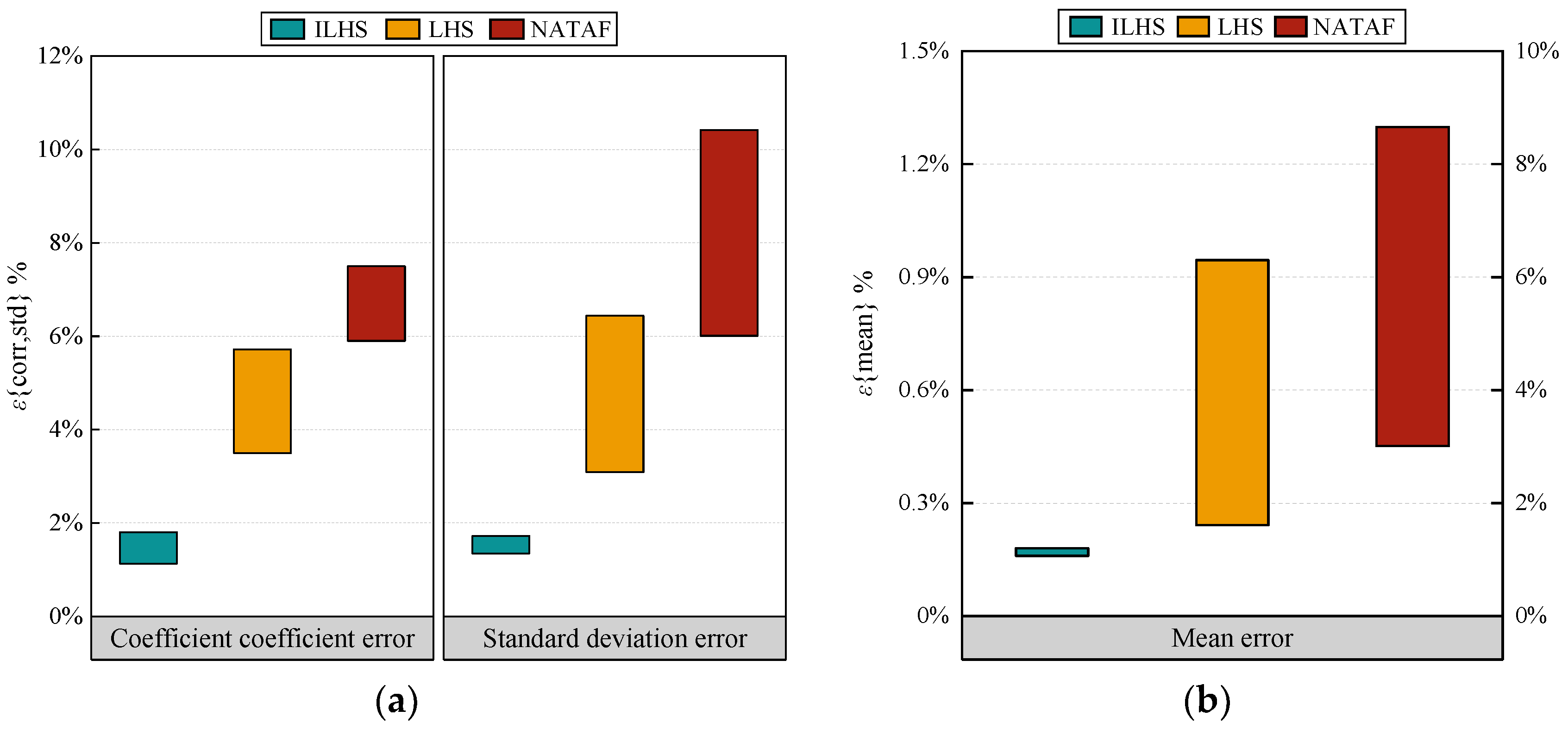
The actual hourly wind speed and solar irradiance of six different observation sites with high renewable energy reserves in China were selected as the sample datasets. The relative error indexes were utilized for these data sets to measure the accuracy of the proposed algorithm. Figure 3 reveals the deviation results in probabilistic information for random variables in 100 replicate experiments with the same sample size to avoid possible fortuity in the test results.

Two common simulation methods are established as a control group to judge the superiority of the proposed algorithm in terms of sampling accuracy. The first control group adopts the Latin hypercube algorithm with adaptive kernel density estimation to describe the correlation among random variables, known as the LHS method. Another control group uses the Nataf algorithm to pass the correlation coefficient among the actual samples.

The effectiveness of the proposed algorithm is demonstrated by comparing the accuracy of the ILHS, the LHS, and the Nataf algorithm. Figure 3a shows the correlation coefficient error of the ILHS decreased by 63.1% and 74.7% when compared with the LHS and Nataf algorithms, respectively. Meanwhile, in terms of the standard deviation error, the LHS and Nataf are 61.7% and 75.4% larger than the proposed method, respectively. It should be noted that, in Figure 3b, the biaxial diagram reveals a significant difference in the value of the evaluation indicators. The left axis of Figure 3b indicates the error range of ILHS and the right axis denotes the error range of LHS and NATAF. The ILHS algorithm can reduce the mean error to 0.18%, which is far less than 2.57% of the corresponding error value of the conventional LHS algorithm.

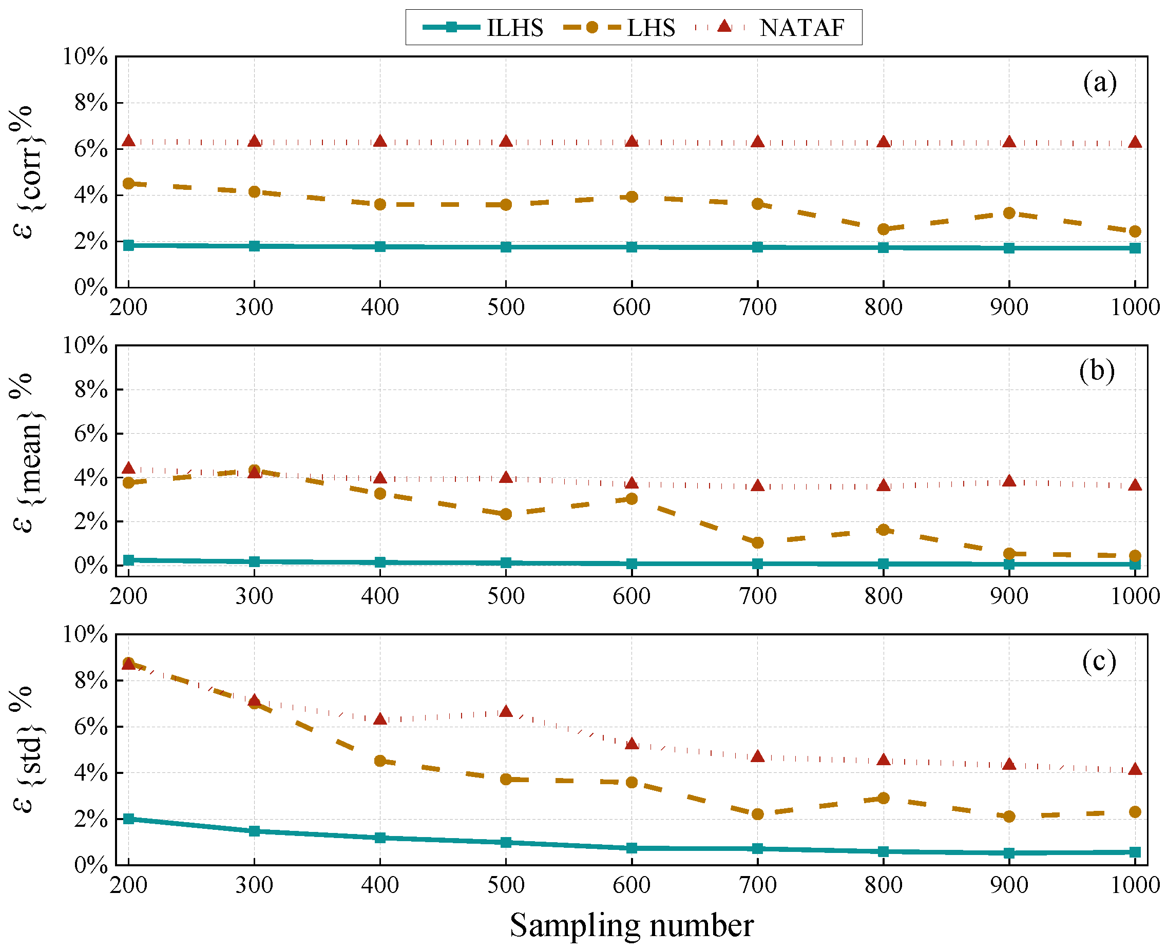
For the robustness test of the algorithm, an experiment was designed to compare the operational accuracy under different sampling numbers, as shown in Figure 4. With the increase in the sampling scale, the mean and standard deviation error of the ILHS showed a minor reduction, while the other two algorithms showed an oscillatory decreasing trend. From the perspective of the whole change process, the error of the proposed algorithm is maintained between 0.06% and 2.01%. Therefore, even if the number of samples was limited to a low level, the ILHS was still able to retain the statistical characteristics of the actual data sets.

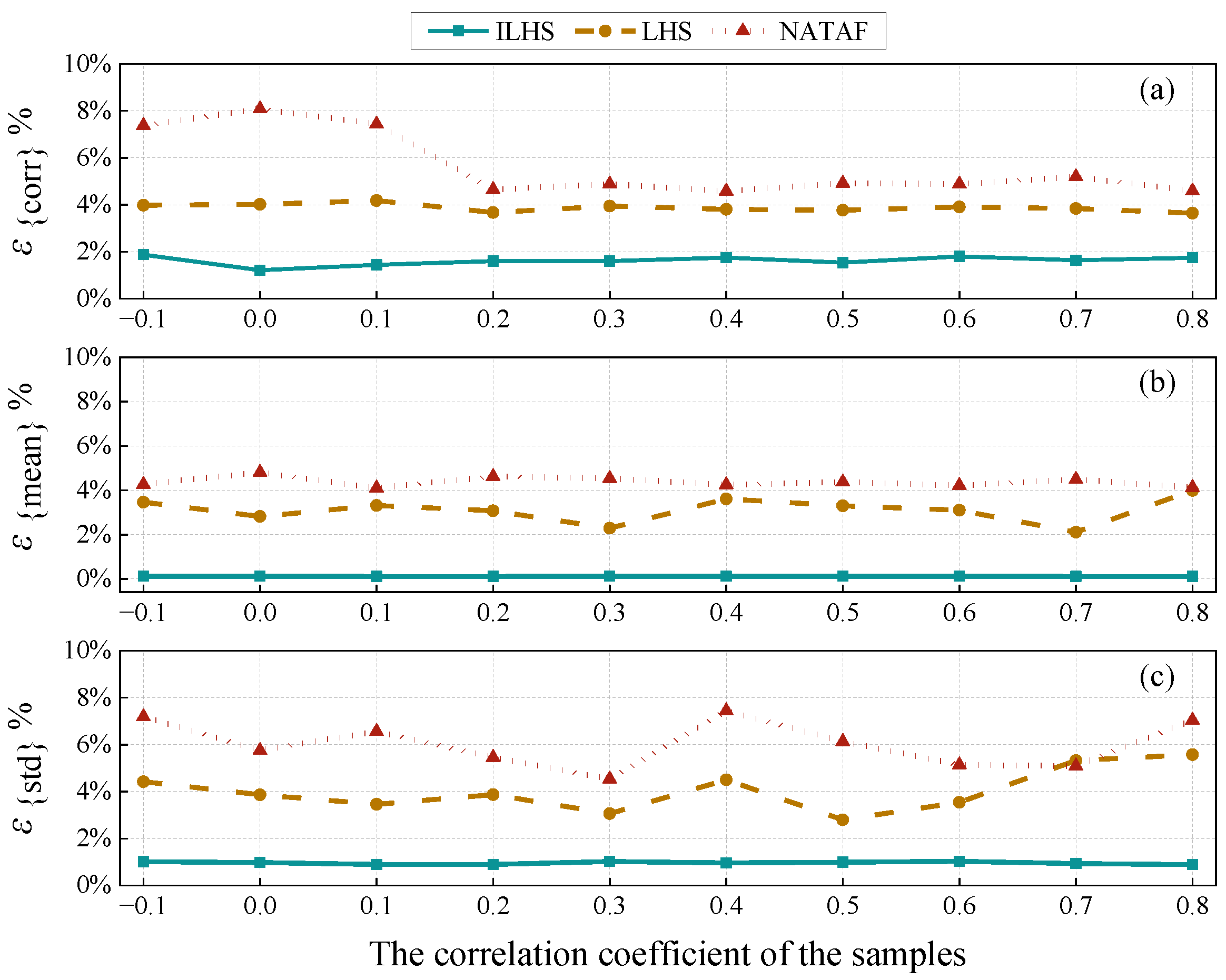
Adequate inheritance of the correlation among actual meteorological data during sampling is the key to ensuring the steady-state analysis accuracy of the power grid with high-penetration renewable energy. Considering that the correlation coefficients between the observation points range from −0.1 to 0.8, the calculation accuracy sensitivity of the different algorithms to the variation of the correlation coefficients is demonstrated in Figure 5.

As the correlation coefficient increases, both the LHS and Nataf algorithms showed major changes, with fluctuations rising to 2.79% and 3.49%, respectively. In contrast, the error fluctuation of the ILHS was stable, in the range of 0.02% to 0.67%. In addition, the results show that the correlation coefficient accuracy of the LHS and Nataf methods is poor when the correlation coefficient is in the range of −0.1 to 0.1. This is because the meteorological data are either uncorrelated or weakly correlated, which makes the sample points of the discrete distribution exhibit irregular changes that reduce the accuracy of the ordinary random sampling algorithm. In contrast, the ILHS combined with the van der Waerden scores can assign reasonable weight values to the upper and lower bounds in the sample to ensure that the model sample sequence is closer to the original data.

According to the performance test results of the ILHS, the proposed algorithm shows good robustness and can significantly fit the correlation and statistical characteristics of the original data with lower sampling times. Furthermore, this algorithm can be applied as an efficient scenario simulation method to fully extract the spatial and temporal complementary characteristics among REs during power flow analysis.

4.2. The Performance Evaluation of the Proposed Method

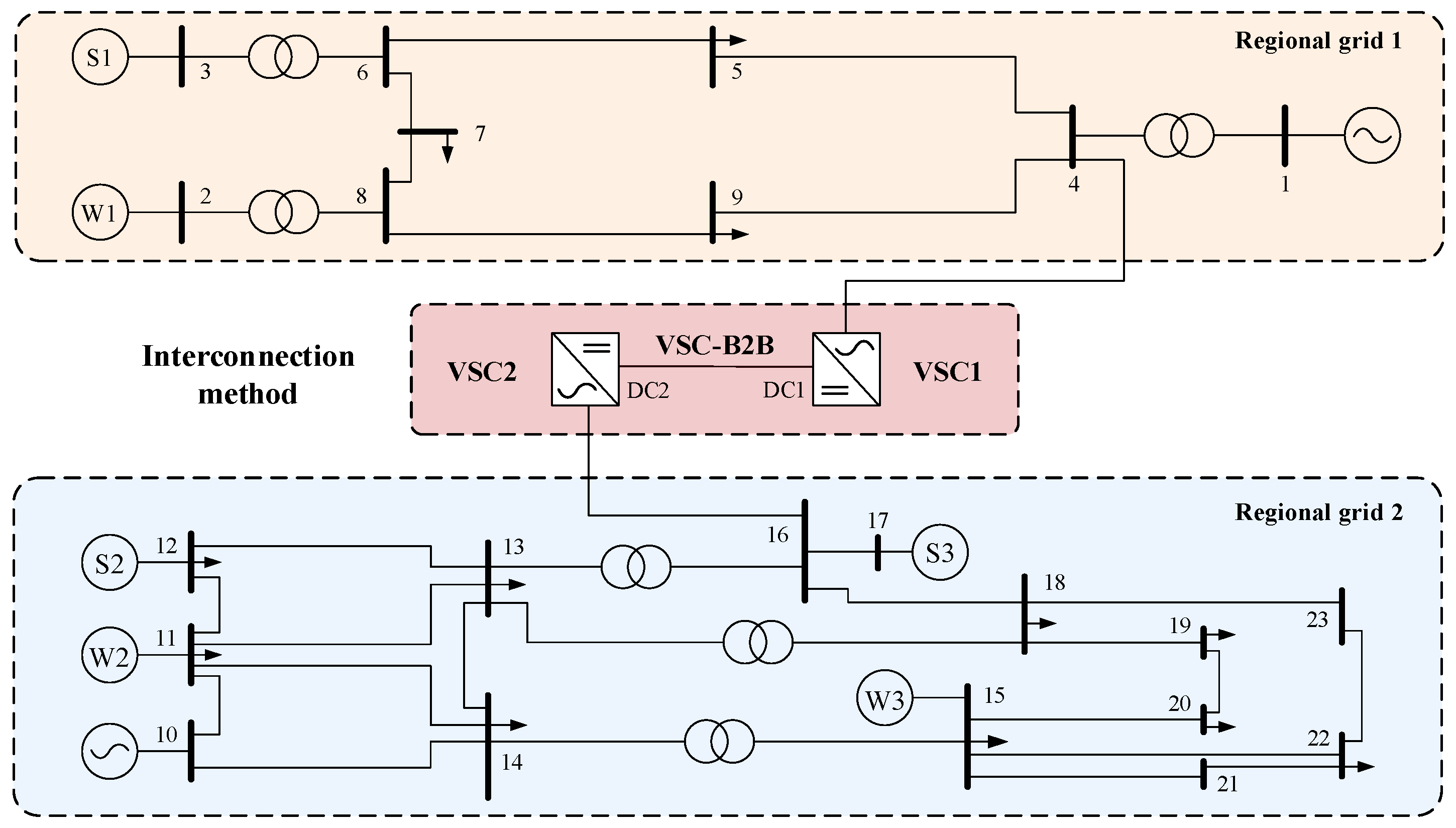
To effectively reduce the fluctuation problems arising from the large-scale renewable energy grid connection, it is necessary to use B2B-VSC structures to connect different regional grids. Therefore, an interconnected grid is constructed by combining IEEE 9-bus and IEEE 14-bus to test the accuracy of the proposed algorithm, as shown in Figure 6. Note that the installed capacity of the six renewable energy power plants connected to the grid is 200 MW, and the base voltage is 345 kV. The capacity base value of the system is set to 100 MW. The relevant settings of the VSC stations are shown in

Table 1. The parameters of converter stations.

	VSC1	VSC2
Ztf/p.u.	0.0015 + 0.1121j	0.0015 + 0.1121j
Bf/p.u.	0.0887	0.0887
Zc/p.u.	0.0001 + 0.1643j	0.0001 + 0.1643j
Control models	Ps1 − Qs1	Udc2 − Us2
Control parameters/p.u.	Ps1 = 1.2 Qs1 = 0.4	Udc2 = 1.0 Us2 = 1.01

.

The wind farm W1 and the photovoltaic (PV) plant S1 are connected to bus 2 and bus 3 in the regional grid 1. The wind farms W2 and W3 and the PV plants S2 and S3 are connected to bus 11, bus 15, bus 12, and bus 17, respectively. The cut-in, rated, and cut-out wind speeds of the individual wind turbine in the wind farm are set at 3.5 m/s, 12 m/s, and 25 m/s, respectively. Photovoltaic panels in the PV farm adopt the structure of a fixed inclination angle.

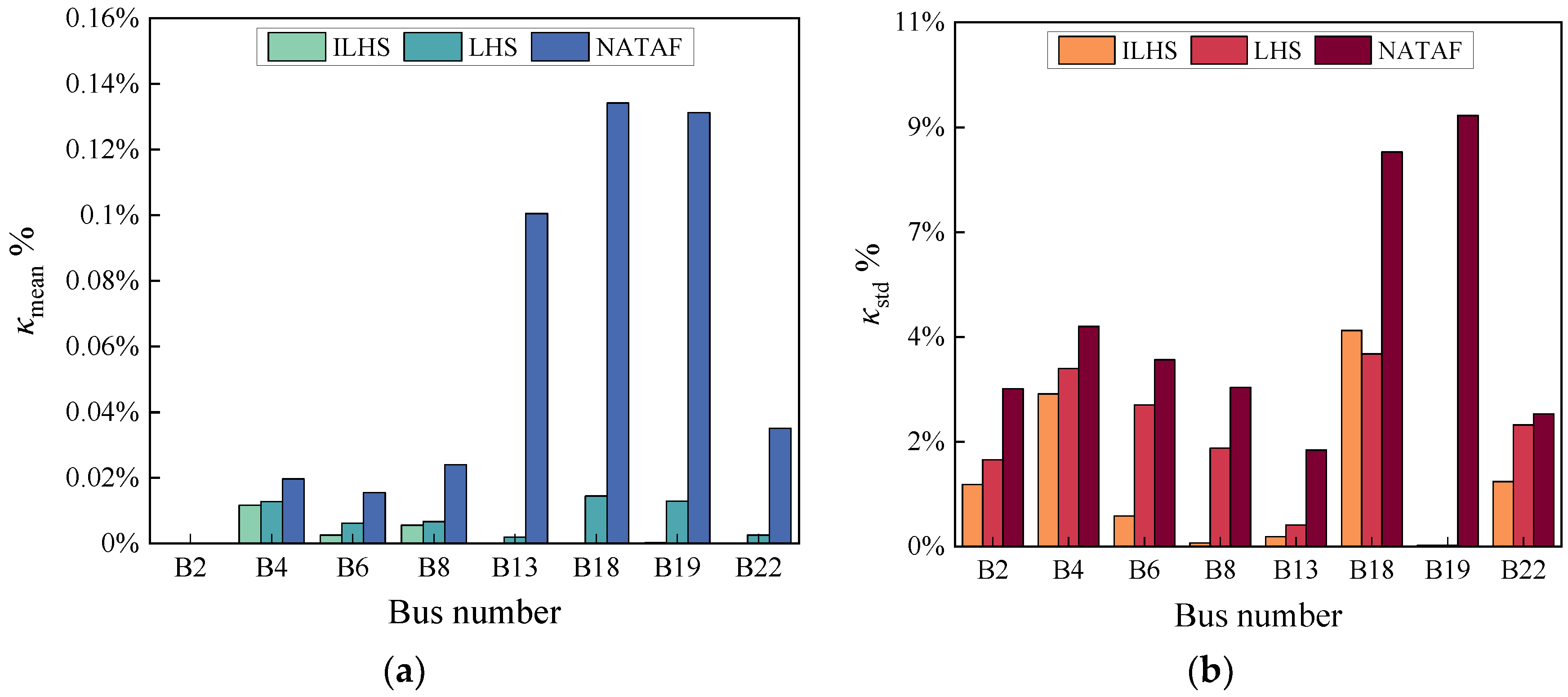
By combining the LHS and Nataf, the accuracy of the proposed method is evaluated in the interconnected grid based on actual meteorological data from renewable resources in China. Figure 7 shows that the ILHS is much more accurate than the other algorithms in terms of the mean and standard deviation of the AC bus voltage magnitude. Compared with the LHS using the stratified median sampling, the mean error of the AC bus voltage magnitude of the proposed method is reduced by 64.9% on average, while the average standard deviation error is reduced by 35.7%. It is worth noting that the LHS and Nataf have a poor approximation of the AC voltage magnitude at part of buses in region 2.

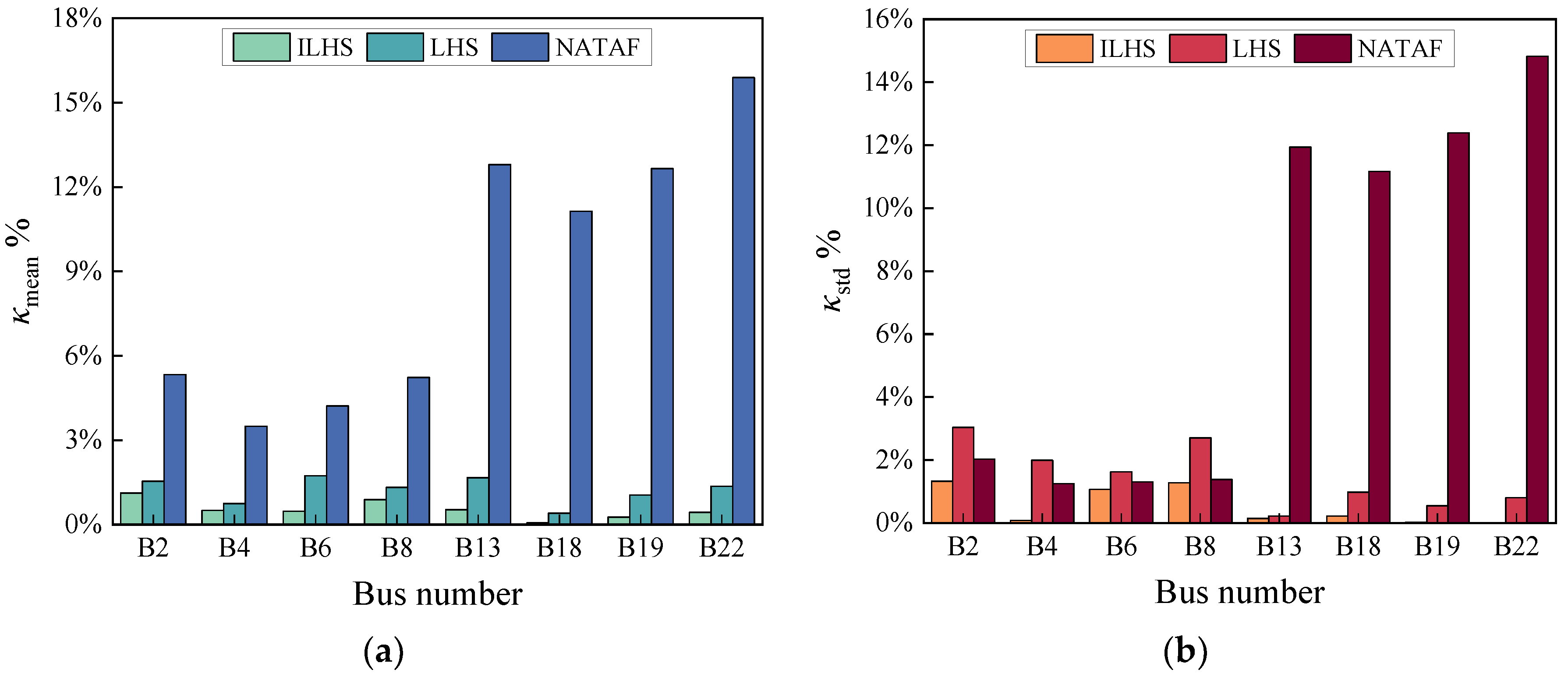
Figure 8 illustrates that the ILHS method has better computational accuracy in terms of the mean and standard deviation of the AC voltage phase angle when compared to the ILHS and the Nataf algorithm, with a maximum error of only 1.12% and 1.32%, respectively. The comparison of the error results in Figure 7 shows that the three PPF methods can better predict the voltage magnitude than the voltage phase angle. Because renewable energy with intermittent nature is connected to the grid, it will aggravate the fluctuation of the active power flowing through each bus. The voltage phase angle difference between the buses reflects the power flow direction. Thus, it increases the difficulty of the PPF in approximating the AC voltage phase angles that exhibit random fluctuations.

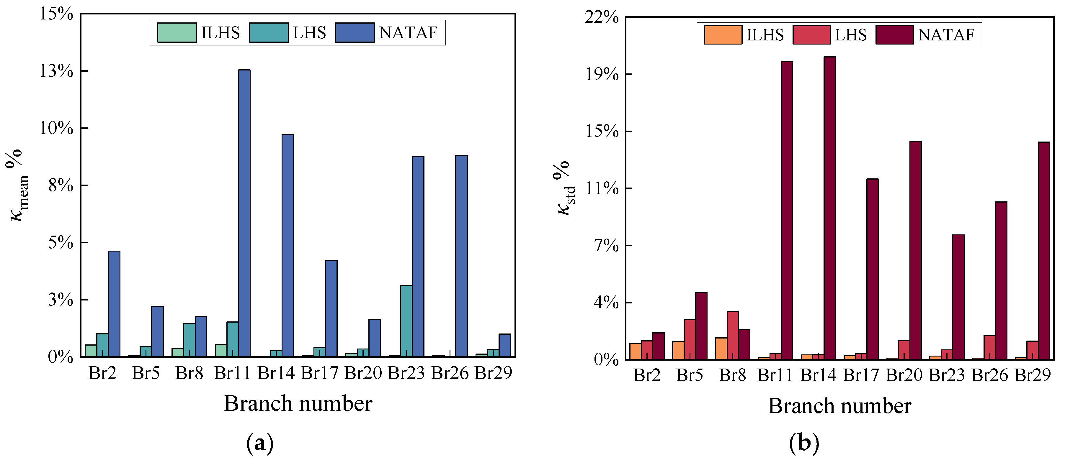
The calculation deviation of the active power in the AC branches through different methods is evaluated in Figure 9. The proposed algorithm, LHS and Nataf, are 0.196%, 0.891%, and 5.53%, respectively, for the average value of the AC active power mean error. Meanwhile, the standard deviations of the AC active power have mean errors of 0.494%, 1.27%, and 10.5%, respectively. By comparing the standard deviation error of the AC active power flowing through the branches in regions 1 and 2, the Nataf in region 2 shows the worst approximation for Br11 and Br14. Region 2 contains more renewable energy stations, and Br11 and Br14 are connected to adjustable power stations. The result is that the Nataf algorithm, which makes specific probability distribution assumptions about random variables, cannot be adapted to the approximate scenario with large fluctuations in the line power.

Considering the importance of the VSC stations in the interconnected grid, the calculation accuracy of different algorithms for the operating parameters at the converter stations is shown in

Table 2. The mean and standard deviation errors of the parameters at the VSC stations.

Test Variables	The Mean Error %			The Standard Deviation Error %
	ILHS	LHS	NATAF	ILHS	LHS	NATAF
Vdc1	0.0024	0.0363	0.0829	0.0122	0.149	25.8
Vca1	0.17	2.45	4.24	0.0565	0.25	23.3
Vca2	0.25	2.86	12.5	0.19	0.28	0.72
Pdc	0.42	2.14	11.8	0.0419	0.097	19.3

. The ILHS method can maintain the calculated deviations of the mean and standard deviation of the relevant variables in the B2B-VSC station at 0.21% and 0.0751%, respectively, which is 88.8% and 61.3% lower than the errors of the corresponding indicators of the LHS method. The Nataf method, that uses conventional probability distribution functions (PDFs) to fit random variables, shows a more obvious disadvantage in the approximate aspect of the relevant variables at VSC stations, with the highest mean and standard deviation of parameter errors reaching 12.5% and 25.8%.

In general, the proposed method demonstrates good operational performance in hybrid AC/DC grids, both for approximating fluctuating random variables and for tracking fixed control variables. In addition, if too many assumptions are considered for the probability distributions of the target variables during the modeling process of the PPF, the simulation results will deviate significantly from the target values due to the inability to accommodate the interference of extreme values in the sampling session.

4.3. The Robustness Evaluation of the Proposed Algorithm

To avoid the limitations of only testing the accuracy of the algorithm in one power grid topology, IEEE 9-bus and IEEE 57-bus were combined to form a new interconnected power grid topology for the test case, as shown in Figure 10. Note that the installed capacity of the six renewable energy power plants connected to the grid is 400 MW. The capacity base value of the system is set to 100 MW. The control parameter settings of the VSC-HVDC stations are shown in

Table 3. The parameter setting of the converter stations.

	VSC1	VSC2
Control models	Ps1 − Qs1	Udc2 − Us2
Control parameters/p.u.	Ps1 = 1.2 Qs1 = 0.2	Udc2 = 1.0 Us2 = 1.004

and the detailed parameters of their internal lines are chosen to be the same as in the previous section.

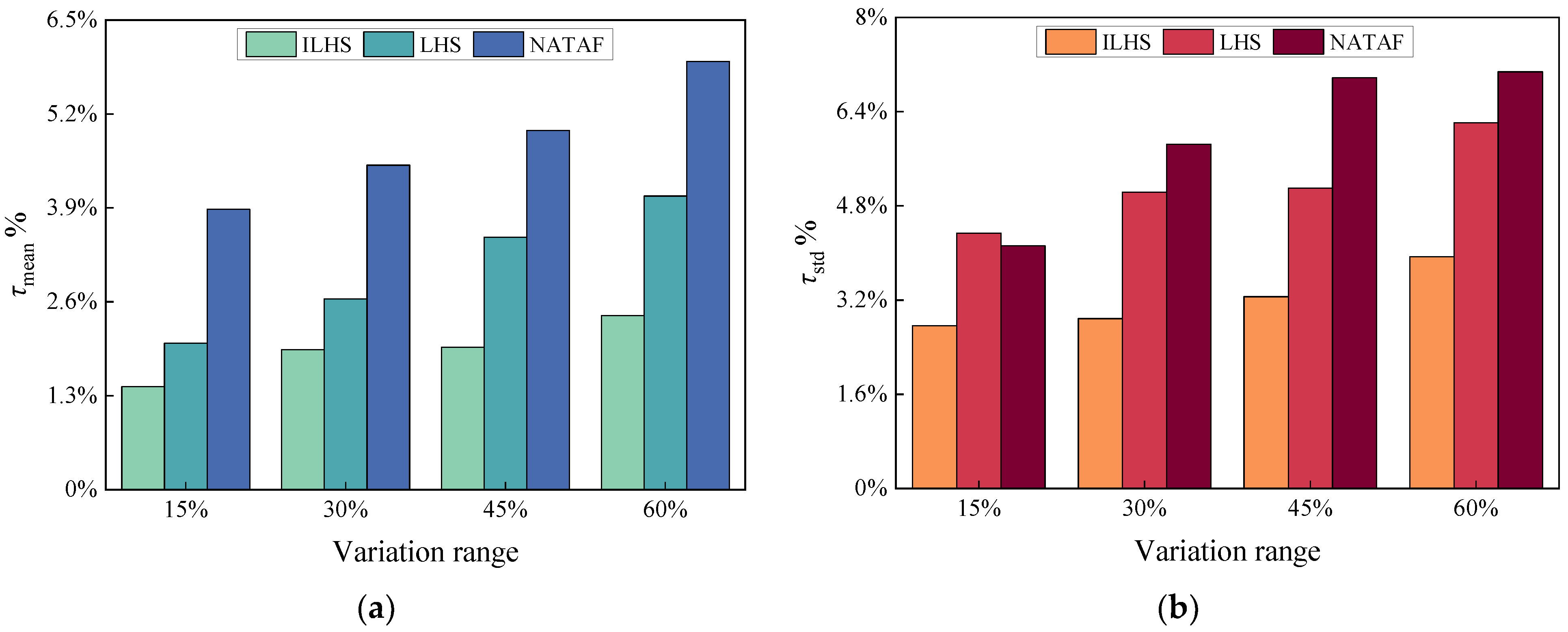
The validity test results of the previous section show that the difficulty of the PPF to approximate the actual value increases as the random variables exhibit more fluctuations during the system operation cycle. Therefore, this subsection first tests whether the proposed algorithm can be adapted to more severe operating scenarios by improving the fluctuation magnitude of the loads in the interconnected grid. Figure 11 demonstrates that the ILHS algorithm can maintain the average mean error and the standard deviation error of the AC voltage magnitude below 0.1% and 2%, respectively, as the power fluctuation range of the load nodes is enhanced from 15% to 60%. In contrast, the maximum error of the Nataf algorithm for the AC voltage amplitude is 4.67%.

Figure 12 proves that the ILHS algorithm is least affected by the increase in the magnitude of the load power fluctuations among the three simulation methods, with the mean error and standard deviation error of the AC voltage phase angle improving by only 0.98% and 1.18% in the different scenarios, respectively. The computational accuracy of the LHS and Nataf algorithms is more sensitive to the variation in the load power fluctuation amplitude. By comparing the calculated errors in Figure 11 and Figure 12, it can be found that the increment in the mean and standard deviation error of the AC voltage phase angle is higher than the mean and standard deviation error of the voltage amplitude during the elevation of the load fluctuation range.

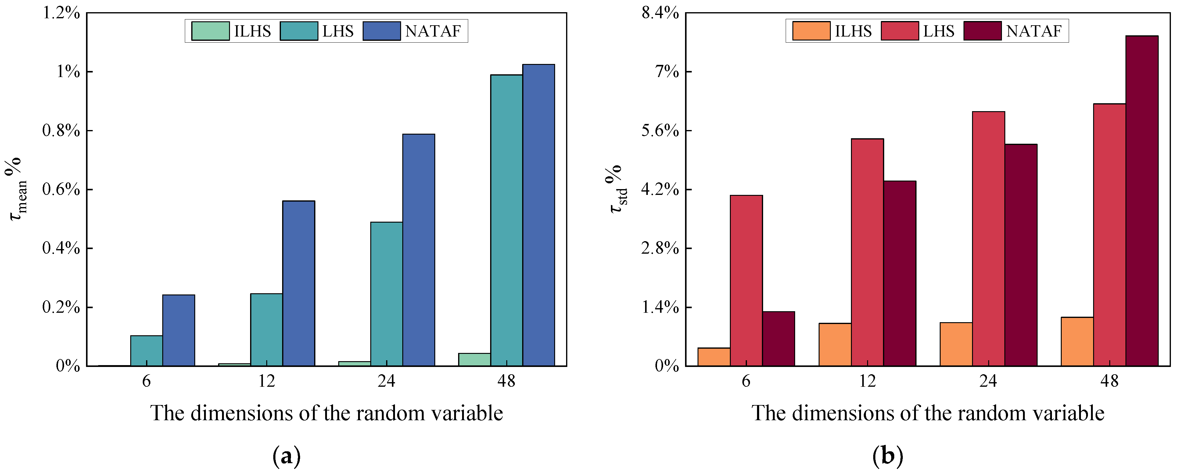
By observing the results of the previous section, it can be concluded that the accuracy of the algorithm will decrease as the number of random variables in the system increases. Therefore, Figure 13 and Figure 14 set up test scenarios with different dimensions of uncertainty variables for evaluating the computational performance of the proposed algorithm in interconnected lines. Figure 13 indicates that even when the dimensionality is raised to 48, the mean and standard deviation errors of the ILHS algorithm for the AC-side power at the converter stations improve to only 0.0000143% and 1.63%, respectively. Interestingly, the three algorithms show very high accuracy in estimating the mean and standard deviation of the active power. Due to the constant active power control used in the VSC1 power plant, the approximate difficulty of the flow power value is reduced.

As seen in Figure 14, the proposed algorithm can maintain the mean and standard deviation of the AC-side voltage phase angle at the converter stations below 0.05% and 1.7%, respectively, in the increasing dimension of the random variables. In addition, by comparing the standard deviation errors of the parameters related to the converter stations in Figure 13 and Figure 14, the performance of the Nataf algorithm is most affected by the change in the dimension of the uncertainty variables, which can increase by up to 8.12%. This is because the Nataf algorithm requires assumptions about the probability distribution of random variables before mapping correlations to the standard normal distribution. When the number of random variables increases, the uncertainty variables cannot be fitted more accurately by relying only on conventional PDFs.

To measure the approximation degree of the PPF to the correlation of uncertain variables, the root mean square error (RMSE) of the correlation coefficients between the AC active power for different random variable dimensions is presented in

Table 4. The root mean square error of the correlation coefficients among the AC active power.

The Dimensions of the Random Variable	The RMSE of Pn
	NATAF	LHS	ILHS
6	0.023	0.02	0.0141
12	0.0417	0.0218	0.0208
24	0.0507	0.0288	0.0226
48	0.0607	0.0403	0.0252

[32]. The RMSE of the Nataf and LHS algorithms increased by a maximum of 2.41 and 1.6 times, respectively, compared to the proposed algorithm during the increment of the random variable dimension. Moreover, the increase in the dimensionality of the uncertainty variables has the most significant enhancement on the RMSE of the active power in the Nataf algorithm, with an error expansion ratio of 264%.

Overall, when compared with the other two PPFs, the ILHS algorithm can guarantee the accuracy of the calculation results and the anti-disturbance of the arithmetic errors in both the load fluctuation amplitude change test and the random variable dimension increment test. Meanwhile, the ILHS algorithm combined with the van der Waerden scores and DKDE can better transfer the correlation among the state variables in a high proportion of renewable energy grids, even in high-dimensional scenarios with input variables.

5. Conclusions

This paper proposes an ILHS algorithm that combined the van der Waerden scores and DKDE. It is intended to solve the problems of extreme rank in intermittent renewable energy meteorological datasets and the inability to accurately fit the marginal distribution of samples using the prior distribution model. This method can ensure the accuracy of the calculation in severe computing scenarios. The conclusions are drawn as follows:

(1)

In terms of the approximate accuracy of sample statistics, the proposed method far exceeds the LHS and the Nataf. At the same time, the ILHS algorithm can still maintain the fitting accuracy in the range of 0.015% to 2.01% in the error test of sample size reduction and the robustness test of dataset correlation change.

(2)

The effectiveness of the proposed method is evaluated in the case of an interconnected grid consisting of IEEE 9-bus and IEEE 14-bus. During the comparison with the calculation errors of the LHS and Nataf algorithms, the ILHS method shows greater approximation accuracy for the AC state variables and the VSC stations’ related variables.

(3)

The computing performance of the proposed algorithm under different severe scenarios is investigated in a modified IEEE 66-bus test system based on the B2B-VSC structure. The ILHS algorithm can ensure that the accuracy is maintained and least disturbed among the three algorithms even when the magnitude of the load fluctuations and the dimensionality of the random variables increase.

The hybrid AC/DC PPF algorithm proposed in this paper can handle random variables with different meteorological characteristics, relying on only a few data points to preserve the statistical properties of the samples and the correlations of the state variables in the nonlinear system of equations. Furthermore, this algorithm provides a probabilistic modeling approach that can reduce the computational difficulties caused by the increased dimensionality of uncertain variables in the optimal scheduling of new power systems and the optimal configuration of energy storage capacity.

References

1. Bouckaert, S.; Pales, A.F.; McGlade, C.; Remme, U.; Wanner, B.; Varro, L.; D’Ambrosio, D.; Spencer, T.; Hosker, E.; Justus, D. (Eds.) Net Zero by 2050—A Roadmap for the Global Energy Sector, 4th ed.; International Energy Agency: Paris, France, 2021.
2. Pennock, S.; Coles, D.; Angeloudis, A.; Bhattacharya, S.; Jeffrey, H. Temporal complementarity of marine renewables with wind and solar generation: Implications for GB system benefits. Appl. Energy 2022, 319, 119276. [Google Scholar] [CrossRef]
3. Drucke, J.; Borsche, M.; James, P.; Kaspar, F.; Pfeifroth, U.; Ahrens, B.; Trentmann, J. Climatological analysis of solar and wind energy in Germany using the Grosswetterlagen classification. Renew. Energy 2021, 164, 1254–1266. [Google Scholar] [CrossRef]
4. Long, B.; Jeong, T.W.; Lee, J.D.; Jung, Y.C.; Chong, K.T. Energy Management of a Hybrid AC-DC Micro-Grid Based on a Battery Testing System. Energies 2015, 8, 1181–1194. [Google Scholar] [CrossRef] [Green Version]
5. Hosseinzadeh, M.; Salmasi, F.R. Robust Optimal Power Management System for a Hybrid AC/DC Micro-Grid. IEEE Trans Sustain. Energy 2015, 6, 675–687. [Google Scholar] [CrossRef]
6. Gabbar, H.A.; El-Hendawi, M.; El-Saady, G.; Ibrahim, E.N.A. Supervisory controller for power management of AC/DC microgrid. In Proceedings of the 2016 IEEE International Conference on Smart Energy Grid Engineering (SEGE), Oshava, ON, Canada, 21–24 August 2016; pp. 147–152. [Google Scholar] [CrossRef]
7. Liu, B.X.; Lund, J.R.; Liao, S.L.; Jin, X.Y.; Liu, L.J.; Cheng, C.T. Optimal power peak shaving using hydropower to complement wind and solar power uncertainty. Energy Convers. Manag. 2020, 209, 112628. [Google Scholar] [CrossRef]
8. Schindler, D.; Schmidt-Rohr, S.; Jung, C. On the spatiotemporal complementarity of the European onshore wind resource. Energy Convers. Manag. 2021, 237, 114098. [Google Scholar] [CrossRef]
9. Mazzeo, D.; Matera, N.; De Luca, P.; Baglivo, C.; Congedo, P.M.; Oliveti, G. A literature review and statistical analysis of photovoltaic-wind hybrid renewable system research by considering the most relevant 550 articles: An upgradable matrix literature database. J. Clean. Prod. 2021, 295, 126070. [Google Scholar] [CrossRef]
10. Li, H.; Zhang, Z.; Yin, X.G. A Novel Probabilistic Power Flow Algorithm Based on Principal Component Analysis and High-Dimensional Model Representation Techniques. Energies 2020, 13, 3520. [Google Scholar] [CrossRef]
11. Ramadhani, U.H.; Shepero, M.; Munkhammar, J.; Widen, J.; Etherden, N. Review of probabilistic load flow approaches for power distribution systems with photovoltaic generation and electric vehicle charging. Int. J. Electr. Power Energy Syst. 2020, 120, 106003. [Google Scholar] [CrossRef]
12. Sun, Y.F.; Xia, D.P.; Gao, Z.C.; Wang, Z.H.; Li, G.Q.; Lu, W.H.; Wu, X.G.; Li, Y. Probabilistic load flow calculation of AC/DC hybrid system based on cumulant method. Int. J. Electr. Power Energy Syst. 2022, 139, 107998. [Google Scholar] [CrossRef]
13. Misurovic, F.; Mujovic, S. Numerical Probabilistic Load Flow Analysis in Modern Power Systems with Intermittent Energy Sources. Energies 2022, 15, 2038. [Google Scholar] [CrossRef]
14. Singh, V.; Moger, T.; Jena, D. Uncertainty handling techniques in power systems: A critical review. Electr. Power Syst. Res. 2022, 203, 107633. [Google Scholar] [CrossRef]
15. Abbasi, A.R. Comparison parametric and non-parametric methods in probabilistic load flow studies for power distribution networks. Electr. Eng. 2022, 104, 3943–3954. [Google Scholar] [CrossRef]
16. Allahvirdizadeh, Y.; Galvani, S.; Shayanfar, H.; Moghaddam, M.P. Risk-averse scheduling of an energy hub in the presence of correlated uncertain variables considering time of use and real-time pricing-based demand response programs. Energy Sci. Eng. 2022, 10, 1343–1372. [Google Scholar] [CrossRef]
17. Wang, W.; Huang, Y.F.; Yang, M.; Chen, C.Y.; Zhang, Y.M.; Xu, X.M. Renewable energy sources planning considering approximate dynamic network reconfiguration and nonlinear correlations of uncertainties in distribution network. Int. J. Electr. Power Energy Syst. 2022, 139, 107791. [Google Scholar] [CrossRef]
18. Zhang, D.L.; Jiang, S.Y.; Liu, J.X.; Wang, L.Z.; Chen, Y.C.; Xiao, Y.X.; Jiao, S.C.; Xie, Y.; Zhang, Y.; Li, M.C. Stochastic Optimization Operation of the Integrated Energy System Based on a Novel Scenario Generation Method. Processes 2022, 10, 330. [Google Scholar] [CrossRef]
19. Galvani, S.; Mohammadi-Ivatloo, B.; Nazari-Heris, M.; Rezaeian-Marjani, S. Optimal allocation of static synchronous series compensator (SSSC) in wind-integrated power system considering predictability. Electr. Power Syst. Res. 2021, 191, 106871. [Google Scholar] [CrossRef]
20. Zhu, J.Z.; Zhang, Y. Probabilistic load flow with correlated wind power sources using a frequency and duration method. IET Gener. Transm. Distrib. 2019, 13, 4158–4170. [Google Scholar] [CrossRef]
21. Mei, F.; Zhang, J.T.; Lu, J.X.; Lu, J.J.; Jiang, Y.H.; Gu, J.Q.; Yu, K.; Gan, L. Stochastic optimal operation model for a distributed integrated energy system based on multiple-scenario simulations. Energy 2021, 219, 119629. [Google Scholar] [CrossRef]
22. Xie, Y.L.; Xu, Y. Transmission Expansion Planning Considering Wind Power and Load Uncertainties. Energies 2022, 15, 7140. [Google Scholar] [CrossRef]
23. Cai, J.L.; Hao, L.L.; Xu, Q.S.; Zhang, K.Q. Reliability assessment of renewable energy integrated power systems with an extendable Latin hypercube importance sampling method. Sustain. Energy Technol. Assess. 2022, 50, 101792. [Google Scholar] [CrossRef]
24. Cao, J.; Du, W.J.; Wang, H.F.F.; Bu, S.Q. Minimization of Transmission Loss in Meshed AC/DC Grids With VSC-MTDC Networks. IEEE Trans. Power Syst. 2013, 28, 3047–3055. [Google Scholar] [CrossRef]
25. Aleixo, S.M.; Teles, J. Weighting Lower and Upper Ranks Simultaneously Through Rank-Order Correlation Coefficients. In Proceedings of the 18th International Conference on Computational Science and Its Applications (ICCSA), Melbourne, VIC, Australia, 2–5 July 2018; pp. 318–334. [Google Scholar] [CrossRef]
26. Botev, Z.I.; Grotowski, J.F.; Kroese, D.P. Kernel Density Estimation Via Diffusion. Ann. Stat. 2010, 38, 2916–2957. [Google Scholar] [CrossRef] [Green Version]
27. Jani, H.K.; Kachhwaha, S.S.; Nagababu, G.; Das, A. Temporal and spatial simultaneity assessment of wind-solar energy resources in India by statistical analysis and machine learning clustering approach. Energy 2022, 248, 123586. [Google Scholar] [CrossRef]
28. Khorramdel, B.; Chung, C.Y.; Safari, N.; Price, G.C.D. A Fuzzy Adaptive Probabilistic Wind Power Prediction Framework Using Diffusion Kernel Density Estimators. IEEE Trans. Power Syst. 2018, 33, 7109–7121. [Google Scholar] [CrossRef]
29. Zhang, J.; Fan, L.Q.; Zhang, Y.; Yao, G.; Yu, P.J.; Xiong, G.J.; Meng, K.; Chen, X.P.; Dong, Z.Y. A Probabilistic Assessment Method for Voltage Stability Considering Large Scale Correlated Stochastic Variables. IEEE Access 2020, 8, 5407–5415. [Google Scholar] [CrossRef]
30. Jithendranath, J.; Das, D.; Guerrero, J.M. Probabilistic optimal power flow in islanded microgrids with load, wind and solar uncertainties including intermittent generation spatial correlation. Energy 2021, 222, 119847. [Google Scholar] [CrossRef]
31. Nosratabadi, H.; Mohammadi, M.; Kargarian, A. Nonparametric Probabilistic Unbalanced Power Flow with Adaptive Kernel Density Estimator. IEEE Trans. Smart Grid. 2019, 10, 3292–3300. [Google Scholar] [CrossRef]
32. Alzubaidi, M.; Hasan, K.N.; Meegahapola, L. Impact of Probabilistic Modelling of Wind Speed on Power System Voltage Profile and Voltage Stability Analysis. Electr. Power Syst. Res. 2022, 206, 107807. [Google Scholar] [CrossRef]
Figure 1. Equivalent diagram of power exchange process in AC/DC hybrid power grid. Numbers 1 to 3 represent the internal structure equivalent diagram of the AC power grid, converter station, and DC power grid, respectively.
Energies 16 02547 g001
Figure 2. Flow chart of improved PPF algorithm.
Energies 16 02547 g002
Figure 3. The error test results of the three algorithms: (a) the correlation coefficient error, standard deviation error; and (b) the mean error.
Energies 16 02547 g003
Figure 4. The variation curve of the error under different sampling scales: (a) the correlation coefficient error; (b) the mean error; and (c) the standard deviation error.
Energies 16 02547 g004
Figure 5. The effect of samples with different correlation coefficients on the accuracy of algorithms: (a) the correlation coefficient error; (b) the mean error; and (c) the standard deviation error.
Energies 16 02547 g005
Figure 6. The topology of the interconnected grid based on the B2B-VSC.
Energies 16 02547 g006
Figure 7. Comparison of (a) the mean error and (b) the standard deviation error of the AC bus voltage magnitudes.
Energies 16 02547 g007
Figure 8. Comparison of (a) the mean error and (b) the standard deviation error of the AC bus voltage phase angles.
Energies 16 02547 g008
Figure 9. Comparison of (a) the mean error and (b) the standard deviation error of the AC branch active powers.
Energies 16 02547 g009
Figure 10. The new topology of the interconnected power grid.
Energies 16 02547 g010
Figure 11. Comparison of (a) the mean error and (b) the standard deviation error of the AC bus voltage magnitudes under different fluctuation ranges of each load.
Energies 16 02547 g011
Figure 12. Comparison of (a) the mean error and (b) the standard deviation error of the AC bus voltage phase angles under different fluctuation ranges of each load.
Energies 16 02547 g012
Figure 13. Comparison of (a) the mean error and (b) the standard deviation error of the active power at the converter stations under different random variable dimensions.
Energies 16 02547 g013
Figure 14. Comparison of (a) the mean error and (b) the standard deviation error of the AC-side bus voltage phase angles at the converter stations under different random variable dimensions.
Energies 16 02547 g014