Article

Research on Production Performance Prediction Model of Horizontal Wells Completed with AICDs in Bottom Water Reservoirs

1
CNOOC China Ltd., Shenzhen Branch, Shenzhen 518067, China
2
MOE Key Laboratory of Petroleum Engineering, China University of Petroleum, Beijing 102249, China
*
Author to whom correspondence should be addressed.
Energies 2023, 16(6), 2602; https://doi.org/10.3390/en16062602
Submission received: 12 January 2023 / Revised: 18 February 2023 / Accepted: 8 March 2023 / Published: 9 March 2023
(This article belongs to the Special Issue Multi-Phase Flow in Wellbore and Machine Learning Optimization Method)

Abstract

:
With the advancement of completion technology for horizontal wells in bottom water reservoirs, Autonomous Inflow Control Devices (AICDs), which have achieved good results in recent years, have been widely used in the oil fields of the eastern South China Sea. Although some mathematical methods can be used to predict the production performance of horizontal wells, there is no dynamic prediction method for the production performance of horizontal wells completed with AICDs. In this work, a mathematical model of porous flow in the reservoir, nozzle flow in the AICD, and pipe flow in the horizontal well is established, and then a new model is presented for predicting the dynamic performance of horizontal wells completed with AICDs in bottom water reservoirs. The new coupling model is compared with two horizontal wells completed with AICDs in the bottom water reservoirs of the eastern South China Sea, and the results indicate that the accuracy of the new model is sufficiently high to provide theoretical support for the further prediction of horizontal wells in the eastern South China Sea.

1. Introduction

Bottom water breakthrough presents many problems and challenges in the efficient development of horizontal wells in the bottom water reservoirs of the eastern South China Sea, which can be solved by controlling the influx of reservoir fluid into the wellbore using different completions [1]. The Inflow Control Device (ICD) is a kind of water control completion installed along the horizontal well in the bottom water reservoir to counteract the non-uniform inflow, hence improving oil recovery. Studies have shown that ICD techniques can be classified as passive inflow control, but the effect diminishes as the water cut increases, especially in the middle and late stages of production. In order to solve this problem, Autonomous Inflow Control Devices (AICDs) have been widely used as a new generation of water control completion technology that is also a passive inflow control device, similar to the ICD. After bottom water breakthrough, it can independently adjust the pressure difference along the horizontal wellbore according to the change in water content to restrain bottom water coning [2,3,4].
The South China Sea is a critical strategic area that has enormous potential for offshore oil and gas exploration and production. The majority of oil wells in the area were developed using horizontal wellbore technology, which has demonstrated high individual productivity. However, these wells have a relatively short period of water-free oil production, with high water content periods lasting over 90% of the production time. To address this issue, water control development is necessary, and the application of water control devices, such as ICDs and AICDs, has achieved significant results. Nonetheless, due to geological variations and differences in development plans, there is considerable variability in the effectiveness of these devices between different production wells. Completion parameters should, therefore, be customized to suit the unique geological conditions and development plans. At present, there is little professional AICD optimization design software available. This study presents a dynamic production prediction model for bottom water reservoirs that can optimize the design of ICDs and AICDs, specify scientific completion plans, and enhance oil recovery rates.
Since the mid-1990s, different types of ICDs, such as the tube, nozzle, and helical path types, have been used for water control in bottom water reservoirs [5]. The first AICD was installed in Norway in 2008 and was used extensively in the Troll field in 2013 with good results [6].
AICDs are mainly of the floating disc type or flow channel type.
The floating disc AICD (Figure 1) [7] has been successfully used in more than 200 oil wells. This disc regulates flow through a moving stream of fluid. The greater the flow velocity, the greater the pressure drop in the stream. When the water cut of a horizontal wellbore increases, the flow velocity increases significantly, resulting in a large pressure difference that inhibits bottom water coning.
The other type of AICD is the flow channel type. Oil and water enter from the inlet on both sides and flow out from the nozzle in the middle. The oil phase, being more viscous, tends to choose a shorter path to the nozzle than the water phase. This difference creates a significant pressure drop that greatly reduces the water flow rate through the AICD [8].
The flow performance of ICDs and AICDs represents the relationship between pressure and flow and is the key factor in calculating the effect of ICDs and AICDs. Least et al. performed flow performance testing of a new kind of AICD in single-phase experimental conditions in a viscosity range of 1 mPa·s to 1000 mPa·s [9]. Least et al. tested the flow performance of oil, water, and gas of the Fluidic Diode Autonomous Inflow Control Device Range 3B, which restricts the flow in areas that produce undesirable fluids [10]. They discussed the testing of ICDs and AICDs in steam flow conditions, that is, the pressure and temperature of the SAGD environment. ICD includes both nozzle-type ICDs and tube-type ICDs [11]. Greci et al. carried out erosion testing of the fluidic diode type ICD in a high sand concentration-level environment. The change in flow performance with time was studied as erosion occurred by comparing the performance curves before and after corrosion [12]. Corona et al. measured the multiphase flow performance of the fluidic diode AICD in light-oil reservoirs. It was proved that the fluidic diode AICD is a reliable solution to increase oil recovery with no moving parts [13]. Carlos A et al. described the successful application of AICDs in heavy oil fields [14].
Numerical simulation methods are an effective means of simulating the production dynamics of the horizontal well and offer many advantages. Oliveira studied the coupling between the reservoir and horizontal wells using a 3D geological model developed based on numerical simulation methods [15]. Youngs et al. used a multi-segment well model combined with the ICD flow model to study the ICD dynamic simulation mathematical model and carried out a field-wide application study that illustrates how the model works [16]. Thornton et al. proposed an integrated solution considering both wellbore characteristics and reservoir characteristics of ICDs. This approach can also be used to support new water control technology such as AICDs and ICVs [17]. Eltaher et al. proposed a process for simulating an Autonomous Inflow Control Valve (AICV) in a coupled reservoir and wellbore model that makes possible a quantitative comparison of downhole completion technologies such as ICDs, AICDs, and AICVs [18]. MoradiDowlatabad et al. provided a method to quantify the impacts of ICD and AICD on reservoir uncertainties. The results show that AICD has a better water control effect than ICD [19].
In this paper, we present a production performance prediction model of horizontal wells completed with AICDs in bottom water reservoirs. The new model is an integrated mathematical model coupled with AICDs, horizontal wells, and bottom water reservoirs. Furthermore, we verify the accuracy of the model by using field data of a real horizontal well completed with AICDs and achieve good results.

2. Integrated Coupled Mathematical Model

2.1. Flow Assumptions

Driven by the pressure drop between the bottom water reservoir pressure and the bottom hole flow pressure, the oil–water two-phase liquid in the formation enters the annular space between the wellbore and the completion string at different positions in the horizontal section, and mixes in the annular space, which is separated by packers. Then, the liquid enters the horizontal wellbore through the AICD valve, which provides an additional pressure drop according to different water content. Finally, the liquid flows from the toe of the horizontal well to the heel and is extracted from the ground.
The analysis incorporates the whole process of liquid flowing into the wellbore from the bottom water reservoir to production including multiphase flow in porous media, annulus flow in the wellbore and completion strings, viable mass flow in a horizontal pipe, and orifice flow in the AICD (Figure 2). At the same time, since the distance between the two packers is generally short, in order to simplify the calculation, it is assumed that there is no annular flow pressure drop in the modeling process.

2.2. Reservoir Simulation

Reservoir simulation uses numerical models to predict well production dynamics. It is an important tool for good management and helps reservoir engineers determine the best production strategy by predicting the future oil and water production of a well. A numerical model is created by discretizing the reservoir into different grids and solving by the differential method. It is assumed that the reservoir is a bottom water reservoir with only oil–water two-phase flow, regardless of the influence of gas and the composition of each phase fluid. The material balance equation is [20,21].
v o B o q o = t ϕ S o B o
v w B w q w = t ϕ S w B w
where vo is the seepage velocity of oil, m/s; vw is the seepage velocity of water, m/s; Bo is the volume coefficient of oil, decimal; Bw is the volume coefficient of water, decimal; So is the saturation of oil, decimal; Sw is the saturation of water, decimal; qo is the flow rate of oil in the standard state, m3/s; and qw is the flow rate of water in the standard state, m3/s.
The influence of gravity can be obtained from Darcy’s law:
v o = K K ro μ o p o ρ o g D
v w = K K rw μ w p w ρ w g D
where K is the absolute permeability, 10−3 μm2; Kro is the relative permeability of oil, decimal; Krw is the relative permeability of water, decimal; μo is the viscosity of oil, mPa.s; μw is the viscosity of water, mPa.s; po is the oil phase pressure, MPa; pw is the water phase pressure, MPa; ρo is the density of oil, kg/m3; ρw is the density of water, kg/m3; g is the acceleration of gravity, m/s2; and D is the depth (downward is positive), m.
Substituting Equation (3) into Equations (1) and Equation (4) into Equation (2) gives the seepage equations of the oil and water phases:
K K ro B o μ o p o ρ o g D q o = t ϕ B o S o
K K rw B w μ w p w ρ w g D q w = t ϕ B w S w
Auxiliary equation:
S o + S w = 1
p cow = p o p w
where pcow is the capillary pressure, MPa.
Initial conditions:
p o x , y , z , t t = t 0 = p o 0
S w x , y , z , t t = t 0 = S w 0
where p o 0 is the initial oil phase pressure, MPa; and S w 0 is the initial saturation of water, decimal.
Boundary conditions:
p o n Ω = 0

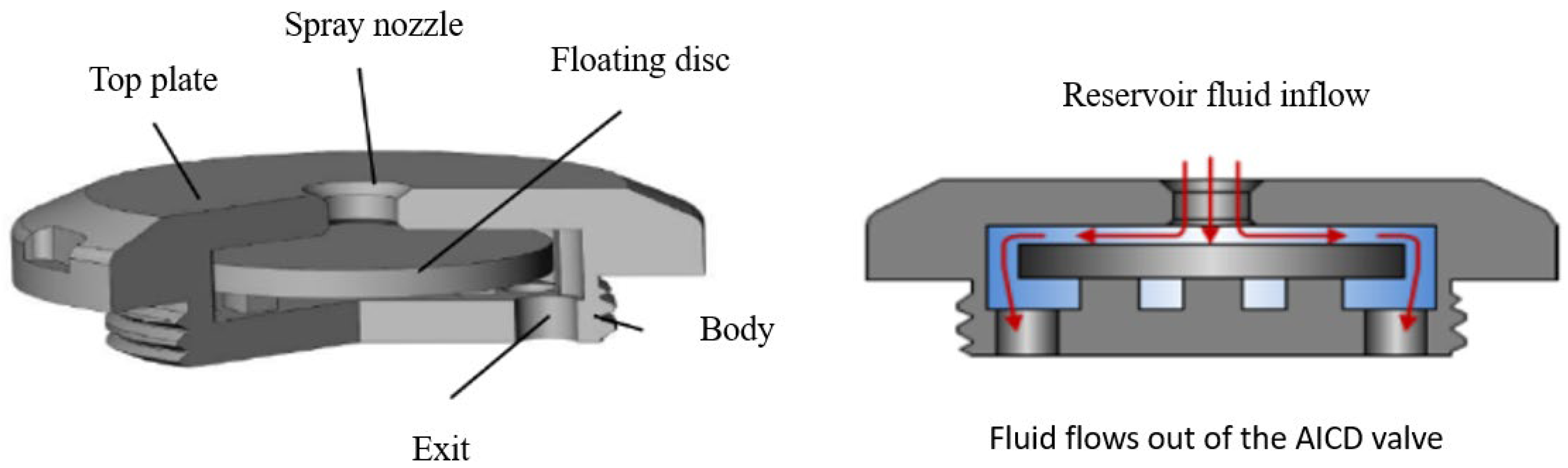
2.3. Flow Performance Model of AICD

Figure 3 shows a floating disc type AICD provided by CNOOC. The flow performance of an AICD is usually obtained using the experimental method. The flow performance data were obtained by conducting experiments and consist of flow rates and pressure drops for different water content (Figure 4).
The flow performance formula of an AICD can be determined by Equation (12) and is represented as (Mathiesen et al., 2011 [22])
Δ P A I C D = K ρ q 2
where ΔPAICD is the pressure drop across the AICD, MPa; q is the volume flow, m3/d; K is the AICD coefficient, dimensionless.
When the properties of the fluid or the water content change, the formula for calculating K is
K = [ ρ m ρ cal ] [ μ cal μ m ] y a AICD
ρ m = f w ρ w + ( 1 f w ) ρ o
μ m = μ o ( 1 f w ) μ w f w
where y is the viscosity index, decimal; aAICD is the AICD control constant, decimal; ρm is the mixture density of oil and water, kg/m3; ρcal is the calibration density, kg/m3; μm is the mixture viscosity of oil and water, mPa.s; μcal is the calibration viscosity, mPa.s; and fw is the water content, decimal.
In the process of fitting the characteristic curve obtained from the experiment, the most important thing is to obtain the aAICD and viscosity index y. This study adopts the following methods to obtain these two key parameters:
(1)
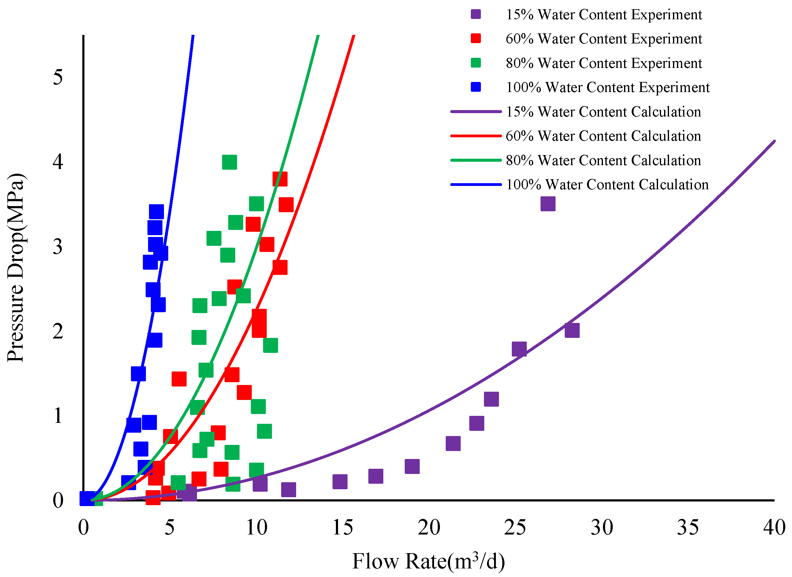
Perform parameter fitting on the characteristic curve of pure water (100% water content)—in this case, the AICD coefficient K is equal to the AICD control constant aAICD—to obtain aAICD.
(2)
Using different viscosity exponents y, the experimental data of different water contents are fitted by Formulas (12)–(15), and the y with the highest fitting degree is selected. Finally, a characteristic curve model suitable for floating disc AICD is obtained.
Using the above method to fit the curves in Figure 5, the coefficients obtained are as shown in Table 1.
Figure 5 presents a comparison between the calculated results of the flow performance curve of the AICD and the experimental results, and consists of a flow rate and pressure drop relationship curve for different water content. It can be seen that the fitted model has high accuracy [23].
This study further simplifies the viscosity index, denoted as y, based on Mathiesen et al.’s formula (Mathiesen et al., 2011). To accommodate fluid mixtures with varying water content, a fitting formula is proposed to fit y with fw. The fitting formula is as follows:
y = a × f w b
where y is the water cut index, decimal; a is the constant, decimal; and b is the water content index, decimal.
Using Equation (16) to fit the curves in Figure 5, the coefficients obtained are as shown in Table 2.

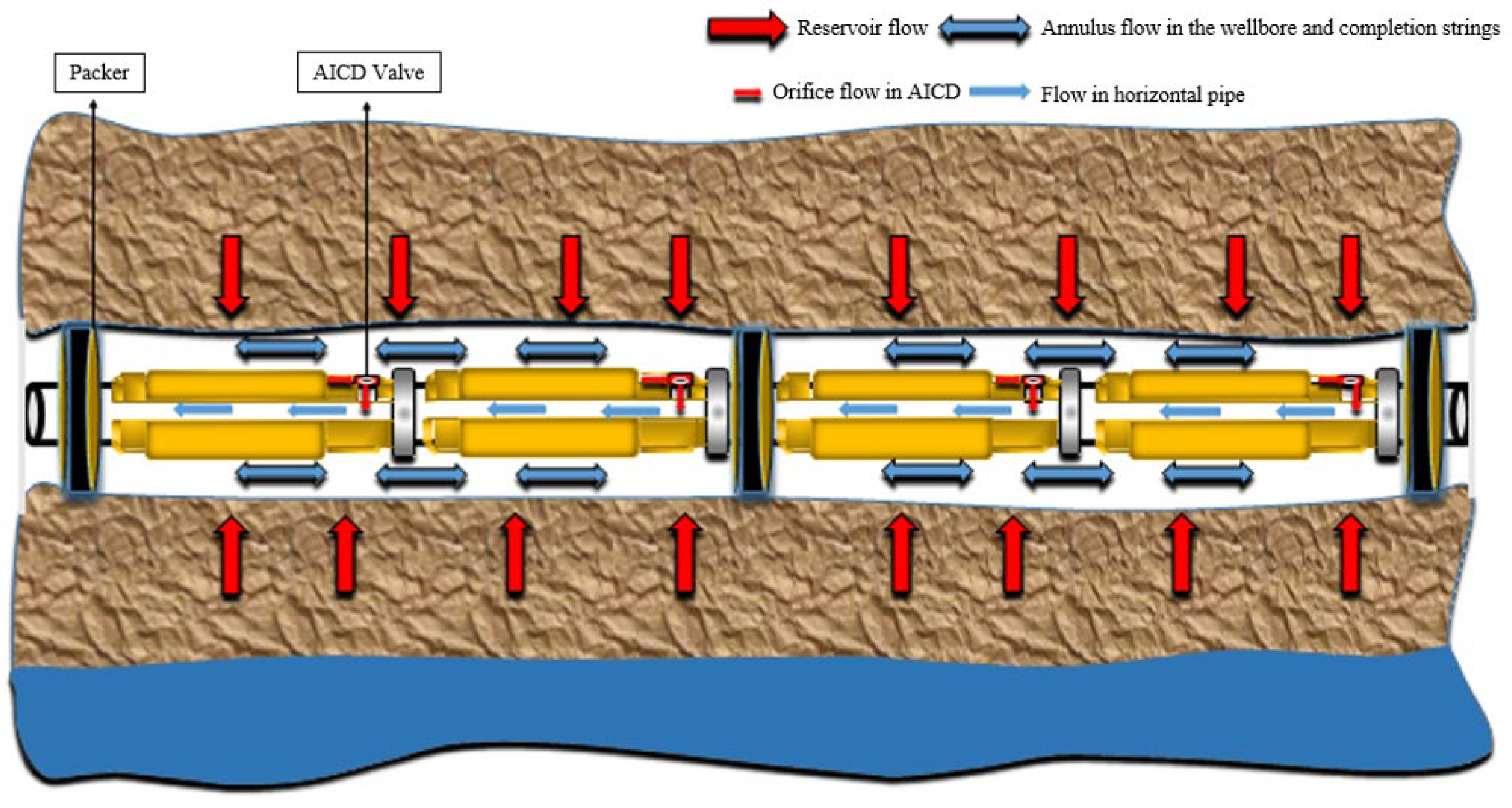
2.4. Flow Model in Horizontal Wellbore

When the two oil–water phases flow from the toe to the heel in the horizontal wellbore, a certain pressure drop will occur. The pressure drop between adjacent well sections can be expressed by the momentum conservation equation, which is written as follows [24]:
P i P i 1 = Δ P h , i + Δ P f , i + Δ P a , i ( i = 2 , 3 , ... , n )
where ΔPh,i is the gravity pressure drop between i − 1 and i, MPa; ΔPa,i is the acceleration pressure drop between i − 1 and i, MPa; and ΔPf,i is the friction pressure drop between i − 1 and i, MPa.

2.5. Model Coupling

A new method based on nodal analysis is presented to couple the flow models of different scales, such as flow in porous media, AICD valve, horizontal wellbore, and horizontal annulus between the wellbore and completion strings.
In order to facilitate the calculation, the block size of the reservoir grid along the horizontal well direction is set as the length of the horizontal wellbore, which has an AICD completion, i.e., each horizontal well section has one connection with a reservoir block and another connection with an AICD completion as shown in Figure 6.
For each time step, we obtain the bottom hole pressure for each horizontal section using the following method.
(1)
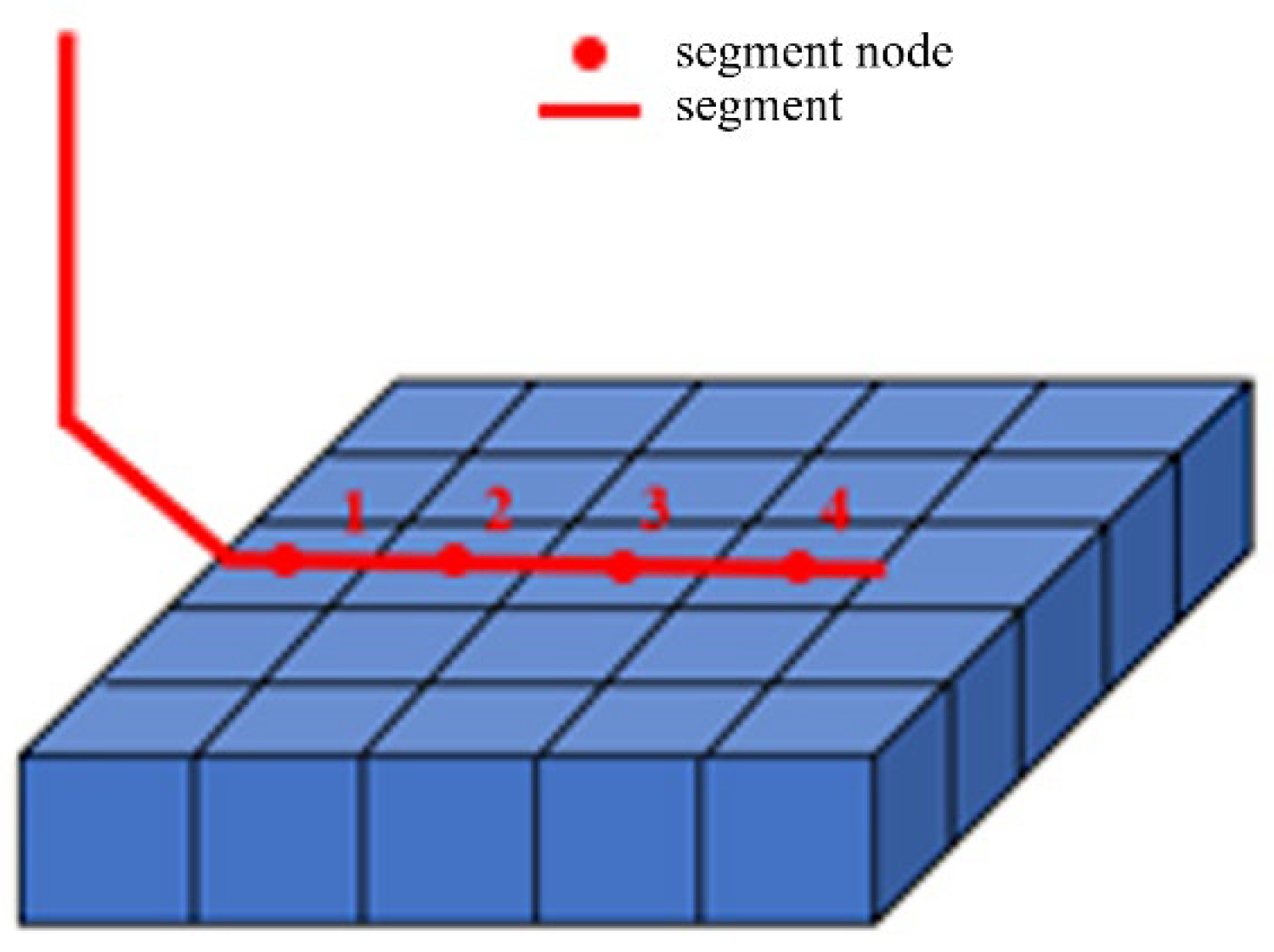
Assume that the packer splits the horizontal well into n segments with m AICDs in each segment.
(2)
For each well segment, assume a series of annular pressures and calculate the oil and water inflow for each segment using the reservoir pressure, saturation, permeability, and well index for that time step.
(3)
Using the flow performance model of AICD, calculate the bottom hole flow pressure corresponding to a series of annular pressures and obtain the relationship between bottom hole flow pressure and oil and water inflow for each well segment.
(4)
Superimpose the production of n segments with the same bottom hole flow pressure to obtain the relationship between total fluid production and bottom hole flow pressure.
(5)
Obtain the corresponding bottom hole flow pressure from step (4) and the annular pressure of each well section from step (3) according to the horizontal well production allocation.
(6)
Input the annular pressure of each well segment from step (5) into the reservoir model as bottom hole flow pressure in an explicit form and calculate the oil and water inflow at that time step.

3. Optimization of the Position of Packers

3.1. Optimization Methods

The isolation of the packer in the annulus between the wellbore and the completion string has an important impact on the water control effect of the horizontal well with AICD completion in a bottom water reservoir. The more packers run in, the better the water control effect will be. However, too many packers installed in the horizontal well can incur huge costs and also increase the engineering risks of construction. In this study, we propose a method for optimizing the running position of the packer based on the permeability distribution.
(1)
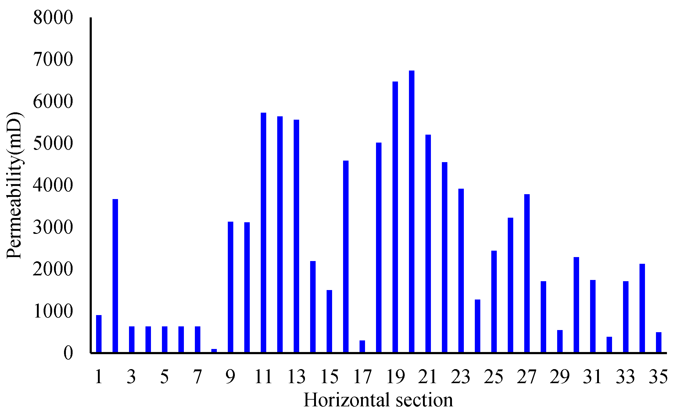
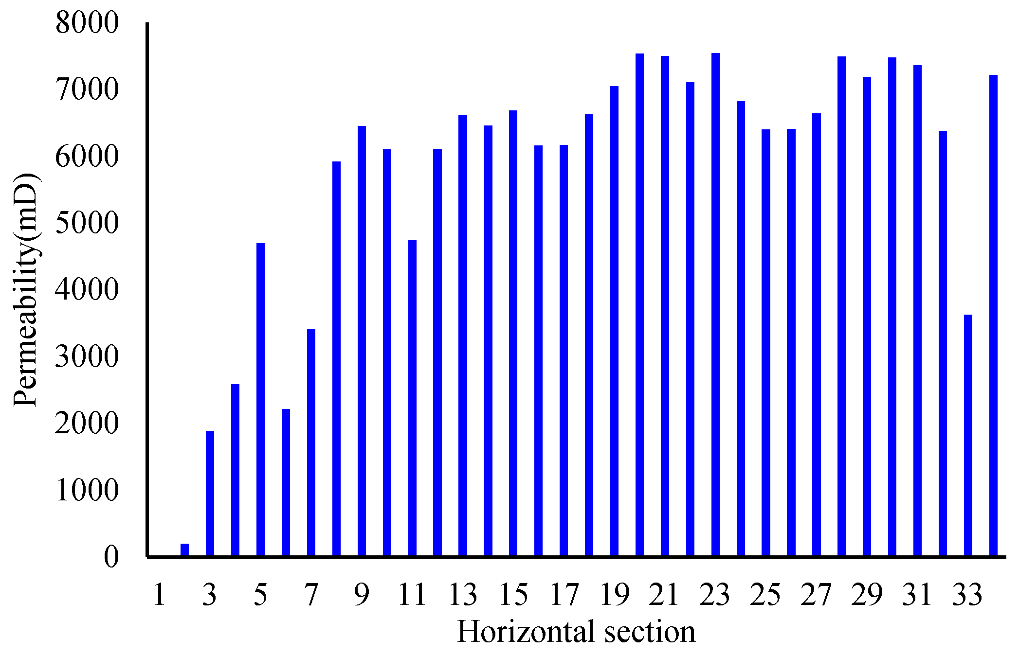
Determine the permeability corresponding to each horizontal well segment.
(2)
Calculate the Ai, T, and Ci values for all adjacent horizontal well segments.
A i = [ K i + 1 K i ] , i = 1 , 2 , , n 1
T = i = 1 n - 1 A i
R i = A i T
where A is the permeability difference of the adjacent horizontal well segments, mD; T is the sum of the permeability differences of all the horizontal well segments, mD; R is the weight of the permeability difference between the adjacent horizontal well segments, decimal; i is the serial number of the horizontal well segment, integer; and n is the total number of horizontal well segments, integer.
(3)
Obtain the order of importance of each packer sorted by Ri.
(4)
Determine the optimal number of packers and optimal position of every packer based on the order of importance of each packer and the actual operating experience.

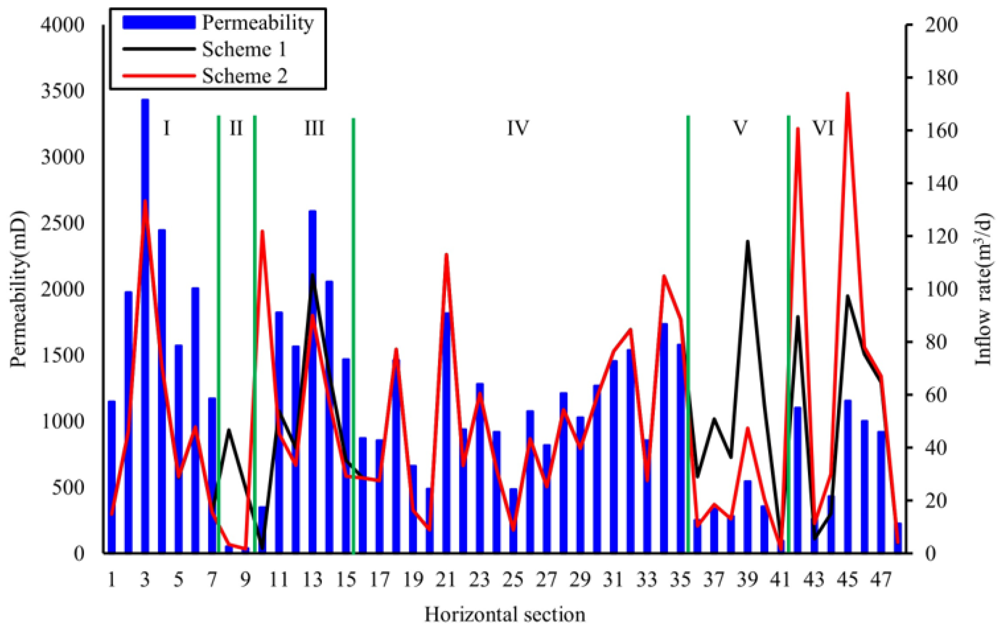
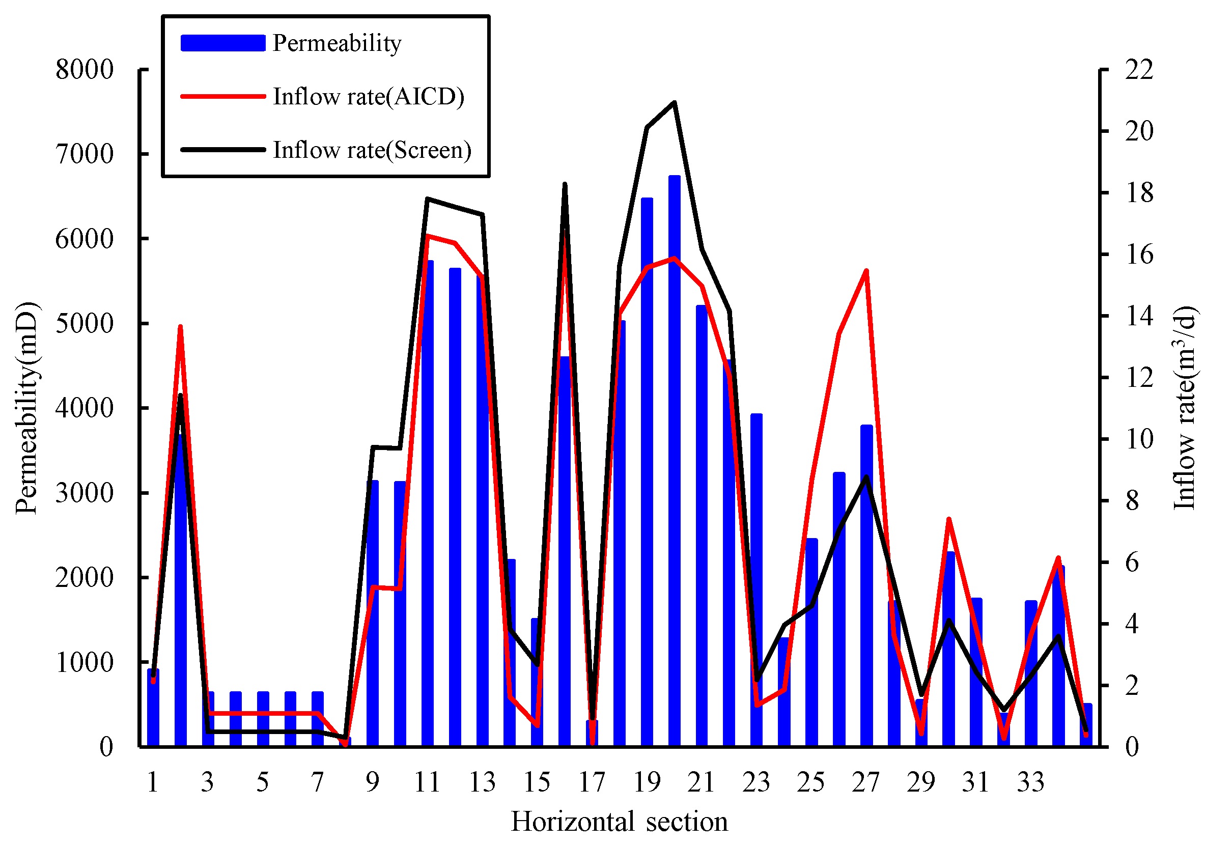
3.2. Optimization Example
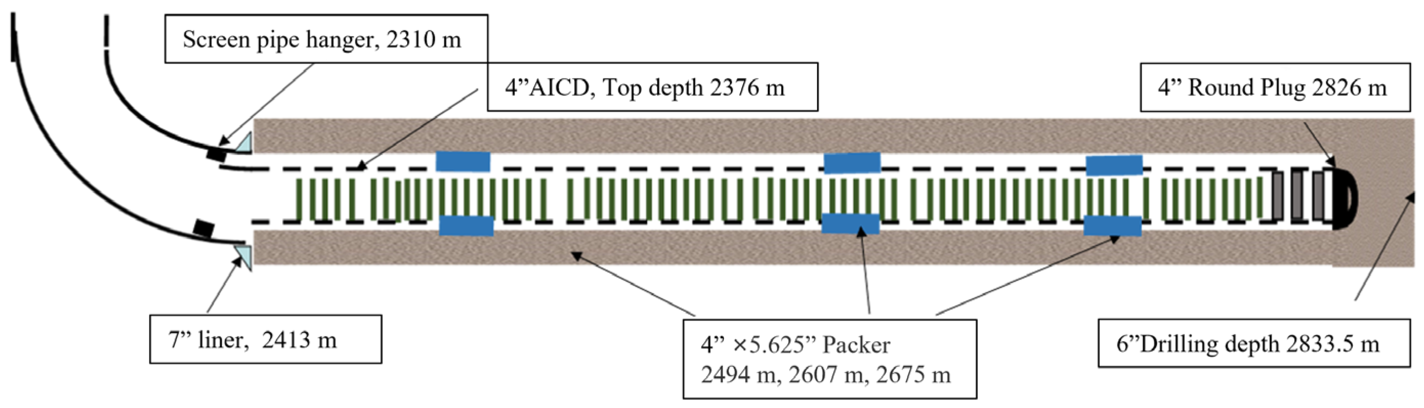
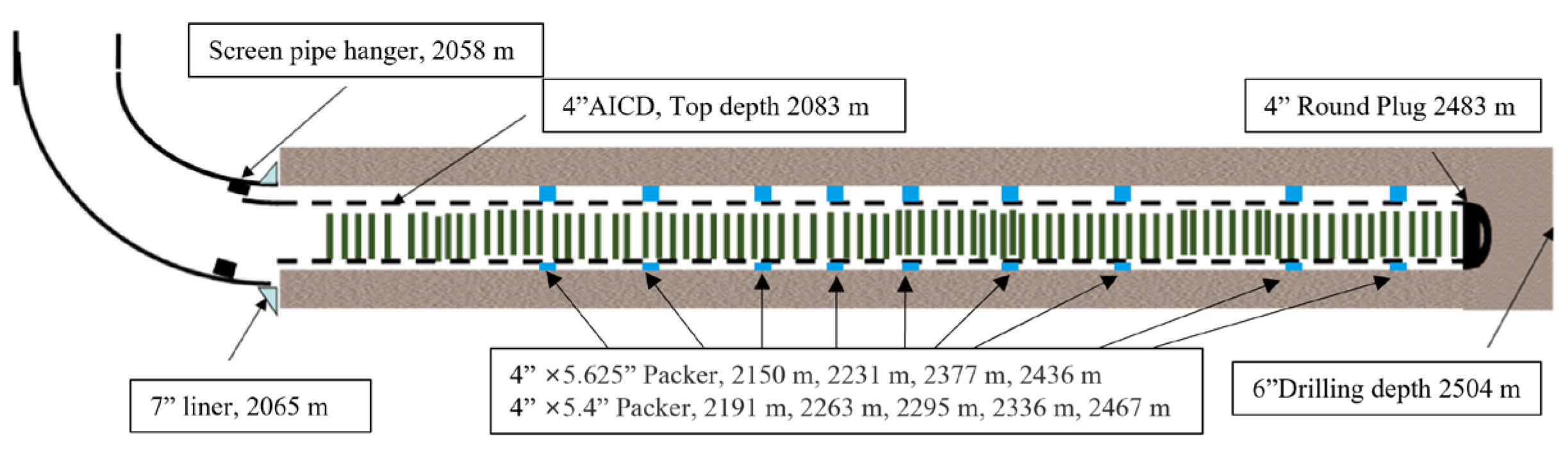
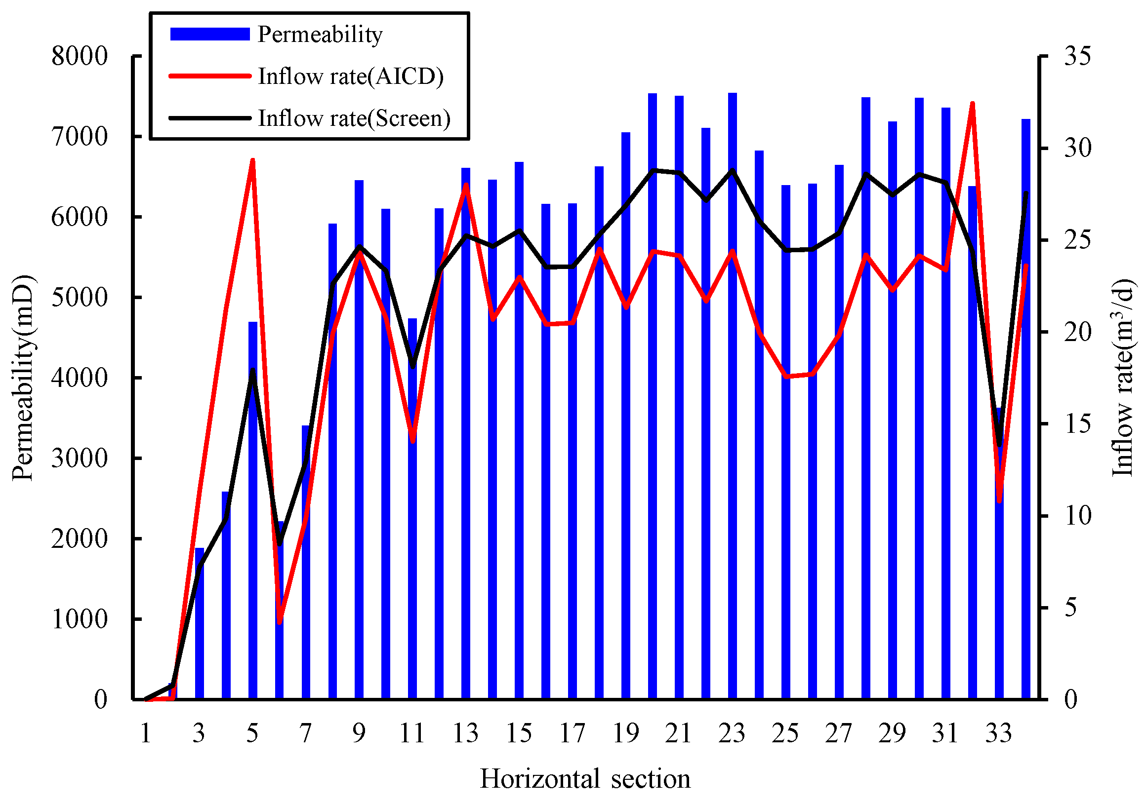
One case has been proposed for the importance of optimizing the position of the packer. As shown in Figure 7, the horizontal well is divided into six sections within zone I to VI, based on the permeability distribution. The distribution illustrates that zones I and III have higher permeability and are susceptible to bottom water coning, therefore requiring a reduction in wellbore inflow to inhibit the coning phenomenon [25].
Two packer position schemes are formulated based on the permeability distribution. As shown in Figure 7, the AICD is denoted by a red circle, the packer is denoted by a black square, and the dashed line represents the zoning of the horizontal well through the packer. The resulting inflow profiles for each design were calculated, and the outcomes of these calculations are shown in Figure 8.
Analysis of the inflow dynamic curve reveals that scheme 1 exhibits a balanced flow curve as shown in Figure 8, providing a favorable liquid lifting effect on zones II and V, while effectively constraining inflow from zone VI and limiting water production. Consequently, the optimal position of packers is instrumental in maintaining the balance of liquid production, underscoring the criticality of packer optimization.

4. Application

Luo et al. and Zhang presented a new semi-analytical model for predicting the performance of horizontal wells completed with ICDs and AICDs, respectively [26]. The semi-analytical model uses a volumetric source to simulate small well sections in a box-type reservoir and connects each small well section back and forth in the form of a horizontal well to obtain an analytic solution for the horizontal well reservoir. The variable mass flow in the horizontal wellbore and the flow in the ICD or AICD are solved by numerical methods. Then, all models are coupled for the solution and an equivalent method is used to simulate different cases of water content. This approach is different from the numerical simulation method used in this study.
There are some commercial software packages that can also simulate horizontal well control completions, the most popular of which are Netool software and Eclipse software. The former uses a static simulation approach, which requires water content prediction based on known permeability distribution and water content saturation distribution. The latter uses a multi-segment well simulation approach (MSW model), which allows dynamic prediction of different water control completion methods.
Therefore, this study compared the Production Performance Prediction Model with the production dynamics of horizontal wells in the eastern region of the South China Sea. As a comparison, we also calculated the production dynamics using Eclipse numerical simulation software.
Two cases were proposed to verify the application of the new model. Two horizontal wells completed with AICDs in the bottom water reservoirs of the eastern South China Sea were used to verify the accuracy of the integrated coupled mathematical model.
Case 1. In this case, the reservoir grid is divided into 80 × 50 × 3. The grid step in the x, y, and z directions is 11.3 m, 50 m, and 1.5 m, respectively. The x-direction is the same as the extension direction of the horizontal well. The length of the horizontal well is 396.2 m, and this is divided into 35 segments, with each horizontal well segment corresponding to an AICD completion. The reservoir parameters are shown in Table 3. The reservoir permeability is shown in Figure 9. The well structure of the horizontal well, which is separated by three packers, is shown in Figure 10.
Figure 11 displays the field water cut and the field oil production of the horizontal well compared to the predicted ones. It can be seen that the model proposed in this paper has high accuracy, reaching 91.2%.
Figure 12 displays the inflow rate on day 200, indicating that both the packer and AICD effectively restrict the flow. The figure highlights the notable limitation of inflow by AICD, which contributes significantly to mitigating bottom water coning.
Case 2. In this case, the reservoir grid system is the same as in Case 1. The total length of the horizontal well in Case 2 is 393.3 m, and this is divided into 34 segments and each horizontal well section corresponds to two AICD completions. The reservoir parameters are shown in Table 4. The reservoir permeability is shown in Figure 13. The well structure of the horizontal well, which is separated by nine packers, is shown in Figure 14.
Figure 15 displays the field water cut and the field oil production of the horizontal well compared to the predicted values. It can be seen that the model proposed in this paper has high accuracy, reaching 93.4%.
Figure 16 displays the inflow rate on day 200, indicating that both the packer and AICD effectively restrict the flow. The figure highlights the notable limitation of inflow by AICD, which contributes significantly to mitigating bottom water coning.
The calculations of the two cases show that the new model can be effectively applied to the production prediction and dynamic analysis of horizontal wells completed with AICDs in the bottom water reservoir in the South China Sea.

5. Conclusions

AICDs have been widely used as a new generation of water control completion technology. To date, there is no effective method to accurately predict its production dynamics.
In this study, a new integrated coupled mathematical model was established based on coupling for the flow in porous media, AICD valve, horizontal wellbore, and the horizontal annulus between the wellbore and completion strings. This model can solve the prediction of a horizontal well completed with AICDs in a bottom water reservoir.
Case studies of two horizontal wells completed with AICDs in a bottom water reservoir were provided in this paper, and the field water cut and field oil production were compared to the predicted values. The accuracy of the model proposed in this work is high enough that it can be applied to the dynamic prediction of horizontal wells in the South China Sea.

Author Contributions

Conceptualization, formal analysis, visualization, project administration, N.Z.; Methodology, validation, writing—review and editing, supervision, Y.A.; writing—original draft, software, data curation, R.H. All authors have read and agreed to the published version of the manuscript.

Funding

This research is part of the National Major Project, “Research on Simulation Method and Evaluation System of a New Type of Water-controlled Completion with Continuous Packer” (CCL2022SZPS0285).

Data Availability Statement

The data used are all included in the paper.

Conflicts of Interest

The authors declare that they have no conflict of interest.

References

  1. Zou, C.; Yang, Z.; He, D.; Wei, Y.; Li, J.; Jia, A.; Chen, J.; Zhao, Q.; Li, Y.; Li, J.; et al. Theory, technology and prospects of conventional and unconventional natural gas. Pet. Explor. Dev. 2018, 45, 604–618. [Google Scholar] [CrossRef]
  2. Li, Q.; Li, Y.; Gao, S.; Liu, H.; Ye, L.; Wu, H.; Zhu, W.; An, W. Well network optimization and recovery evaluation of tight sandstone gas reservoirs. J. Pet. Sci. Eng. 2020, 196, 107705. [Google Scholar] [CrossRef]
  3. Meng, D.; Jia, A.; Ji, G.; He, D. Water and gas distribution and its controlling factors of large scale tight sand gas fields: A case study of western Sulige gas field, Ordos Basin, NW China. Pet. Explor. Dev. 2016, 43, 663–671. [Google Scholar] [CrossRef]
  4. He, D.H.; Bai, B.F. Gas-liquid two phaseflow with high GVF through a horizontal V-Cone throttle device. Int. J. Multiph. Flow 2017, 91, 51–62. [Google Scholar]
  5. Madsen, T. 2 The Troll Oil Development: One Billion Barrels of Oil Reserves Created Through Advanced Well Technology. In Proceedings of the 15th World Petroleum Congress, Beijing, China, 12–16 October 1997. [Google Scholar]
  6. Prakasa, B.; Muradov, K.; Davies, D. Rapid Design of an Inflow Control Device Completion in Heterogeneous Clastic Reservoirs Using Type Curves. In Proceedings of the SPE Offshore Europe Conference and Exhibition, Aberdeen, Scotland, UK, 5–8 September 2015. [Google Scholar]
  7. Shang, B.; Liu, Y.; Meng, X.; Bai, J.; Wu, H.; Yu, F.; Mu, M.; Li, Y. New-Type Water Controlling Technology for Improving Production Performance of Offshore Heavy-Oil Reservoir with Active Bottom Water. In Proceedings of the SPE Annual Technical Conference and Exhibition, Virtual, 28 September–2 October 2020. [Google Scholar]
  8. Michael, F.; Liang, Z.; Least, B. The Theory of a Fluidic Diode Autonomous Inflow Control Device. In Proceedings of the SPE Middle East Intelligent Energy Conference and Exhibition, Manama, Bahrain, 28–30 October October 2013. [Google Scholar]
  9. Brandon, L.; Stephen, G.; Russell, B.; Adam, U.; Wileman, A. Autonomous ICD Single Phase Testing. In Proceedings of the SPE Annual Technical Conference and Exhibition, San Antonio, TX, USA, 8–10 October 2012. [Google Scholar]
  10. Brandon, L.; Stephen, G.; Angel, W.; Ufford, A. Fluidic Diode Autonomous Inflow Control Device Range 3B—Oil, Water, and Gas Flow Performance Testing. In Proceedings of the SPE Kuwait Oil and Gas Show and Conference, Kuwait City, Kuwait, 7–10 October 2013. [Google Scholar]
  11. Least, B.; Greci, S.; Huffer, R.; Rajan, R.V.; Golbeck, H. Steam Flow Tests for Comparing Performance of Nozzle, Tube, and Fluidic Diode Autonomous ICDs in SAGD Wells. In Proceedings of the SPE Heavy Oil Conference-Canada, Calgary, AB, Canada, 10–12 June 2014. [Google Scholar]
  12. Greci, S.; Least, B.; Tayloe, G. Testing Results: Erosion Testing Confirms the Reliability of the Fluidic Diode Type Autonomous Inflow Control Device. In Proceedings of the Abu Dhabi International Petroleum Exhibition and Conference, Abu Dhabi, United Arab Emirates, 10–13 November 2014. [Google Scholar]
  13. Corona, G.; Fripp, M.; Yin, W. Fluidic Diode Autonomous ICD Multiphase Performance in Light-Oil Reservoirs. In Proceedings of the SPE Middle East Oil & Gas Show and Conference, Manama, Bahrain, 18–21 March 2017. [Google Scholar]
  14. Pedroso, C.A.; Rocha, P.; Araujo, Z. Successful AICD Application to Reduce Water Production in a Heavy Oil Greenfield. In Proceedings of the SPE Annual Technical Conference and Exhibition, Houston, TX, USA, 3–5 October 2022. [Google Scholar]
  15. Rodolfo, O. Study of the Horizontal Wellbore and Reservoir Coupling. In Proceedings of the SPE Annual Technical Conference and Exhibition, Denver, CO, USA, 30 October–2 November 2011. [Google Scholar]
  16. Youngs, B.; Neylon, K.; Anthony Holmes, J. Recent Advances in Modeling Well Inflow Control Devices In Reservoir Simulation. In Proceedings of the International Petroleum Technology Conference, Doha, Qatar, 7–9 December 2009. [Google Scholar]
  17. Thornton, K.; Jorquera, R.; Soliman, M.Y. Optimization of Inflow Control Device Placement and Mechanical Conformance Decisions Using a New Coupled Well-Intervention Simulator. In Proceedings of the Abu Dhabi International Petroleum Conference and Exhibition, Abu Dhabi, United Arab Emirates, 11–14 November 2012. [Google Scholar]
  18. Eltazy, E.; Khafiz, M.; David, D.; Grebenkin, I. Autonomous Inflow Control Valves—Their Modelling and “Added Value”. In Proceedings of the SPE Annual Technical Conference and Exhibition, Amsterdam, The Netherlands, 27–29 October 2014. [Google Scholar]
  19. MoradiDowlatabad, M.; Zarei, F.; Akbari, M. The Improvement of Production Profile While Managing Reservoir Uncertainties with Inflow Control Devices Completions. In Proceedings of the SPE Bergen One Day Seminar, Bergen, Norway, 22 April 2015. [Google Scholar]
  20. Zhao, F.K. The Study on Development Law and Effective Drive Strategy of Horizontal Well in Bottom Water Reservoir; China University of Petroleum (East China): Dongying, China, 2018. [Google Scholar]
  21. Guo, D.L.; Liu, C.Q. Two-Phase Flow in a Horizontal Well Penetrating a Naturally Fractured Reservoir Under Bottom Water Drive. Pet. Explor. Dev. 1995, 22, 44–46+101–102. [Google Scholar]
  22. Mathiesen, V.; Aakre, H.; Werswick, B.; Elseth, G. The Autonomous RCP Valve—New Technology for Inflow Control in Horizontal Wells. In Proceedings of the SPE Offshore Europe Oil and Gas Conference and Exhibition, Aberdeen, UK, 6–8 September 2011. [Google Scholar]
  23. Zhu, C.M.; Liu, G.Z.; Li, X.B. Experimental Study on Water Control Performance of New AICD. China Pet. Mach. 2019, 47, 79–86. [Google Scholar]
  24. Wang, X.Q.; Wang, Z.H.; Wei, J.G. Investigation of variable mass flow in horizontal well with perforation completion coupling reservoir. J. Hydrodyn. 2005, 3, 326–331. [Google Scholar]
  25. Sapian, N.F.A.; Tusimin, F.; Mei, S.C.M.; Wang, A.G.J.; Ali, N.A.W.; Madzidah, A.; Ghonim, E.O.; Awid, A.; Hasbullah, N.; Nazim, N.O.M. Maximizing Production Recovery Through Autonomous Inflow Device AICD Configuration in Challenging Long Horizontal Open-Hole Oil Producer with High Gas-Oil-Ratio and Un-Even Fluid Contacts. In Proceedings of the IADC/SPE Asia Pacific Drilling Technology Conference and Exhibition, Bangkok, Thailand, 9–10 August 2022. [Google Scholar]
  26. Zhang, N.; Li, H.; Dong, W.; Cui, X.; Tan, Y. The optimal model of water control completion based on source function and network model. J. Pet. Sci. Eng. 2022, 213, 110398. [Google Scholar] [CrossRef]
Figure 1. Schematic diagram of floating disc AICD (The red arrows represent the direction of reservoir fluid).
Energies 16 02602 g001
Figure 2. Schematic diagram of flow at different spatial scales in horizontal-well AICD completion.
Energies 16 02602 g002
Figure 3. Floating disc AICD.
Energies 16 02602 g003
Figure 4. Comparison between fitted model and experiment.
Energies 16 02602 g004
Figure 5. The fitting effect of the Mathematical model.
Energies 16 02602 g005
Figure 6. Schematic diagram of horizontal well AICD water control completion coupling.
Energies 16 02602 g006
Figure 7. Segmented schematic diagram of different schemes.
Energies 16 02602 g007
Figure 8. Effect of packer position on horizontal well inflow dynamics.
Energies 16 02602 g008
Figure 9. Permeability profile for Case 1.
Energies 16 02602 g009
Figure 10. Horizontal well structure for Case 1 (The packer is indicated by a blue square, the reservoir is indicated by the brown area, and the AICD is indicated by a green square).
Energies 16 02602 g010
Figure 11. Comparison of predicted results with field results for Case 1.
Energies 16 02602 g011
Figure 12. Inflow profile of horizontal well section for Case 1.
Energies 16 02602 g012
Figure 13. Permeability profile for Case 2.
Energies 16 02602 g013
Figure 14. Horizontal well structure for Case 2 (The packer is indicated by a blue square, the reservoir is indicated by the brown area, and the AICD is indicated by a green square.).
Energies 16 02602 g014
Figure 15. Comparison of predicted results with field results for Case 2.
Energies 16 02602 g015
Figure 16. Inflow profile of horizontal well section for Case 2.
Energies 16 02602 g016
Table 1. Coefficients of the flow performance curve of the AICD.
Water ContentyaAICD
15%−12.4610.22
60%−6.26810.22
80%−5.32410.22
100%−3.9810.22
Table 2. Coefficients of the water cut index (y).
ab
−4.525−0.5361
Table 3. Reservoir parameters for Case 1.
ParametersValues
Porosity, %23.4
Stratigraphic pressure, MPa15.06
Saturation pressure, MPa0.4
Stratigraphic temperature, °C74.09
Crude oil density, g/cm30.941
Crude oil viscosity, mPa·s353.5
Table 4. Reservoir parameters for Case 2.
ParametersValues
Porosity, %27.9
Stratigraphic pressure, MPa16.57
Saturation pressure, MPa8.5
Stratigraphic temperature, °C74.85
Crude oil density, g/cm30.941
Crude oil viscosity, mPa·s353.5
Disclaimer/Publisher’s Note: The statements, opinions and data contained in all publications are solely those of the individual author(s) and contributor(s) and not of MDPI and/or the editor(s). MDPI and/or the editor(s) disclaim responsibility for any injury to people or property resulting from any ideas, methods, instructions or products referred to in the content.

