Optimization of the Thermal Environment of Large-Scale Open Space with Subzone-Based Temperature Setting Using BEM and CFD Coupling Simulation

Abstract

A cruise ship, which has large-scale open spaces, has an uneven cabin thermal environment in the cruise public space, leading to overcooling or poor cooling issues. Therefore, optimizing the thermal environment of public spaces during a cruise should be the priority. According to the space functions of the cruise ship, the large public space is divided into three subzones: the entertainment area (Subzone I), the round-table dining area (Subzone II), and the square-table dining area (Subzone III). To create a uniform, stable, and comfortable thermal environment, this study proposes a subzone-based temperature setting approach to independently adjust the thermal environment of each subzone. Coupling simulation of building energy modeling (BEM) and computational fluid dynamics (CFD) was adopted in this study to determine proper temperature setpoints of the subzones under different occupancy rates. The results indicate that, compared with a single-temperature setpoint for the entire public space, the subzone-based temperature setpoints could achieve a uniform thermal environment. The average temperature difference among the three subzones was 0.68 °C. Moreover, the airflow between two adjacent subzones considerably affected the BEM results of energy consumption of the air-conditioning system.

1. Introduction

The air-conditioning system in a cruise ship guarantees a comfortable travel life, and the performance of this system affects not only the travel experience of passengers but also the energy demands of the ship [1,2,3]. However, to date, research on the cabin thermal environment has often been neglected [4]. In public spaces of cruise ships, the density of personnel and the activity levels of occupants vary drastically in different functional areas. Nevertheless, either overcooling or poor cooling commonly occurs in the large open spaces of the cruise, which creates an uncomfortable thermal environment for the personnel and affects the energy efficiency of the air-conditioning system [5]. The thermal environment of public spaces in a cruise needs to be optimized for evaluating effective heat strain indices [6]. Computational fluid dynamics (CFD) has often been used to address indoor environment problems in large open spaces [7,8,9,10]. However, the reliability of CFD simulation results strongly depends on the accurate boundary conditions [11,12,13]. The issue of building energy consumption can be resolved when building energy modeling (BEM) is used [14,15,16,17]. BEM simulates energy consumption using a well-mixed model ignoring the airflow patterns of the space, which is unsuitable for energy consumption simulation for large open spaces with an uneven temperature distribution and a complicated airflow pattern [18].

In 1985, Clarke et al. proposed a combination of BEM and CFD, which opened up the research path for coupled simulation [19,20]. Additionally, applying the conjugate heat transfer method allows the CFD to incorporate the functionality of BEM [21,22]. The conjugate heat transfer method has a wide range of applications and powerful functions, but the computational overhead is particularly large with this method [23]. In 2002, Zhai et al., proposed a coupling simulation with CFD and BEM [24]. The results of that study suggested that the BEM-CFD coupling simulation could compensate for both limitations. BEM provides precise boundary conditions for CFD simulations, and CFD provides accurate airflow information to offset the limitations of BEM simulation in large-space environments. Research on BEM-CFD coupling simulation should pay attention to two important points: (i) what parameters need to be exchanged for the coupling simulation, and (ii) how the parameters need to be exchanged.

For the question of which parameters need to be exchanged for coupling simulation, Negrão et al., in 1998, studied a large space in a building wherein radiators were used for heating [25]. In that study, BEM software was used to output accurate boundary conditions to CFD, which then transmitted airflow characteristics in space to BEM. Rivera et al., reported the heat transfer coefficient extracted from CFD and outputted it to BEM for a more accurate energy consumption estimation [26]. Du et al., passed the load and supplied air temperature and airflow rate from BEM to CFD [27]. Tian et al., summarized the data types exchanged between BEM and CFD in coupled simulation, wherein the information extracted by CFD from BEM included the temperature of the inner wall surface, wind speed, full pressure and temperature of the air outlet, and outdoor climate conditions [28]. The parameters that BEM can obtain from CFD include the wall flow heat transfer coefficient, wall surface temperature or heat flow within the envelope, small-scale climate conditions, mass exchange rate, and other local thermal environment parameters. CFD-BEM coupling simulations have been used in many studies, and the data exchanged between the two software applications are different in each application. The next question is how to exchange parameters between coupled simulations. According to the solution method of the model, Djunaedy et al., divided coupling simulation into two types: internal coupling and external coupling [29]. Internal coupling refers to the use of the same solver for calculations, and before the calculation, the calculation models of BEM and CFD need to be fused; by contrast, external coupling refers to linking two independent and complete calculation models through an intermediate agent. Compared with internal coupling, external coupling is easier to implement. The exchange through external coupling can also be carried out by building an intermediate platform but more often in the form of manual data exchange. Manzandet et al., used manual coupling to study the thermal performance of double-layer skin glass curtain walls. In that study, manual coupling was chosen as a means of data exchange [30].

Another important aspect to consider is how data are synchronized. In 2002, Zhai et al., summarized data synchronization methods into two categories: static coupling and dynamic coupling [24]. Dynamic coupling involves data exchange at each time step in the simulation process, and this process is highly accurate but computationally intensive. Static coupling involves data exchange at a small scale; that is, only a small amount of information is being exchanged between BEM and CFD to solve the respective control equations; although the accuracy is slightly poor, the practicality is stronger. Static coupling is categorized as one-step static, two-step static, and so on, according to the number of data exchanges between the two applications. Considering that the present study requires multiple simulations of the same model, as each time the data are relatively independent, the one-step static data synchronization method is selected.

BEM-CFD coupling simulation is used in many fields. Hien et al., used the CFD-BEM coupling method to study the thermal properties of double-skinned glass curtain walls in regions with tropical climates in Singapore [31]. Yamamoto et al., used the CFD-BEM coupling simulation method to reproduce the temperature distribution in an environment with predominant natural convection of floor heating [32]. Barbason et al., used this coupling simulation method to improve the overheating problem in two-story residential buildings in Belgium [33]. Zhang et al., used the coupling simulation method for constructing a framework and optimized outdoor convection heat transfer modeling in different urban communities [34]. Jonas et al., used the CFD-BEM coupling simulation method to measure air and surface temperatures and reported that the increase in air and surface temperatures was due to the presence of new buildings to mitigate the urban heat island effect [35]. Ascione et al., used the CFD-BEM coupling method to obtain accurate information about the heating, ventilating, and air-conditioning (HVAC) system energy requirement and indoor microclimatic control [36]. Tian et al., used this coupling approach to obtain a holistic solution for designing and operating low-energy buildings [37]. Fan and Ito developed a BEM-CFD coupling simulation approach to study various supply air locations in an office building [38]. Shan et al., used the CFD–EnergyPlus coupling method to study a large-space office in Hong Kong; the results showed that this coupling method could effectively provide low-energy thermal comfort in a large open office environment with multi-terminal unit services [39]. Zhang et al., proposed a coupling framework to integrate a high-resolution CFD model into a coupled low-resolution CFD and BEM model for studying purge cooling of a community night-time building, and the resulting surface coupling method could reduce computational costs [40,41].

Based on the findings of the aforementioned published studies, CFD-BEM coupling can compensate for any limitations encountered in past studies [42,43]. This coupling method can co-optimize the indoor environment and energy consumption of a large open space. In the present study, we proposed a subzone-based temperature setting approach to independently adjust the thermal environment of each subzone, mainly to create a uniform, stable, and comfortable thermal environment. The CFD-BEM coupling simulation method was used to perform multiple coupling simulations of public spaces with various occupant rates. Stepwise temperature adjustment with higher accuracy than that in previous studies resulted in an appropriate subzone-based temperature setpoint to achieve a uniform thermal environment on the cruise ship. It is worth noting that this article also focuses on analyzing the impact of indoor air information on energy consumption estimates. By comparing the estimated results before and after considering the airflow information, the rules for its impact on energy consumption results are obtained.

The sections of this manuscript are structured as follows: Section 2 introduces the subzone-based temperature setpoint setting method and the CFD-BEM coupling framework. Section 3 addresses the models built using BEM and CFD and presents the preliminary simulation results. Section 4 discusses the results of the coupling simulation. Finally, Section 5 presents the conclusions.

2. Methodology

2.1. Subzone-Based Temperature Setpoint Setting Method

In large spaces, the unified temperature setting for the overall area usually causes uneven temperature distribution. Therefore, the subzone-based temperature setpoint setting method was proposed considering space function and occupancy rates.

In this study, the public space in a cruise ship is a typical large-space indoor environment. Considering the different functions of each area, the public space was categorized into three air-conditioned areas, namely the entertainment area (Subzone I), round-table dining area (Subzone II), and square-table dining area (Subzone III). The number of people in Subzone I and Subzone II is limited by the number of tables and chairs and is often constant. To analyze the influence of occupancy rates on the thermal environment, the number of people in Subzone III was changeable. This study considered six cases wherein occupancy rates ranged from 0.25 to 1 (

Table 1. Different occupancy rates in Subzone III.

Case No.	1	2	3	4	5	6
Number of people	135	101	84	66	48	36
Occupancy rates	1	0.75	0.6	0.5	0.35	0.25
Overall occupancy rate	1	0.87	0.81	0.74	0.67	0.63

). Using the BEM-CFD coupled simulation, the appropriate subzone temperature setpoint was obtained under different occupancy rates.

2.2. BEM-CFD Coupled Simulation

The BEM software application used in this study was EnergyPlus 9.6.0, and the CFD simulation software application used was Fluent 16.0. After determining the air conditioning set temperature for each zone using multiple coupling simulations, EnergyPlus outputted the energy consumption of the HVAC system by considering airflow information in the large open space. Considering the time course of each software in this study, the discontinuity in the calculation speed and external coupling was more suitable for this study [29,44,45]. Therefore, the present study adopted a two-way external coupling of BEM and CFD simulations, and the data exchange between the two software applications was performed manually. The overall framework is shown in Figure 1.

The subzone-based temperature setpoint was based on coupling between EnergyPlus and Fluent. First, the zone output variables of EnergyPlus, namely, wall inner face temperature, window inner face temperature, and supply airflow rates, were set as the boundary conditions of CFD simulation. Then, temperature distributions and airflow patterns were determined using CFD simulation, after which the average air temperature of the subzones was compared with that of the subzone temperature setpoint to adjust the subzone temperature settings. Meanwhile, the mass exchange rates between the adjacent subzones were inputted in return to EnergyPlus to simulate energy consumption considering airflow information within the large space. Thus, the integrated optimization of the thermal environment and energy consumption was performed using BEM-CFD coupling simulations.

3. Simulation Case Study

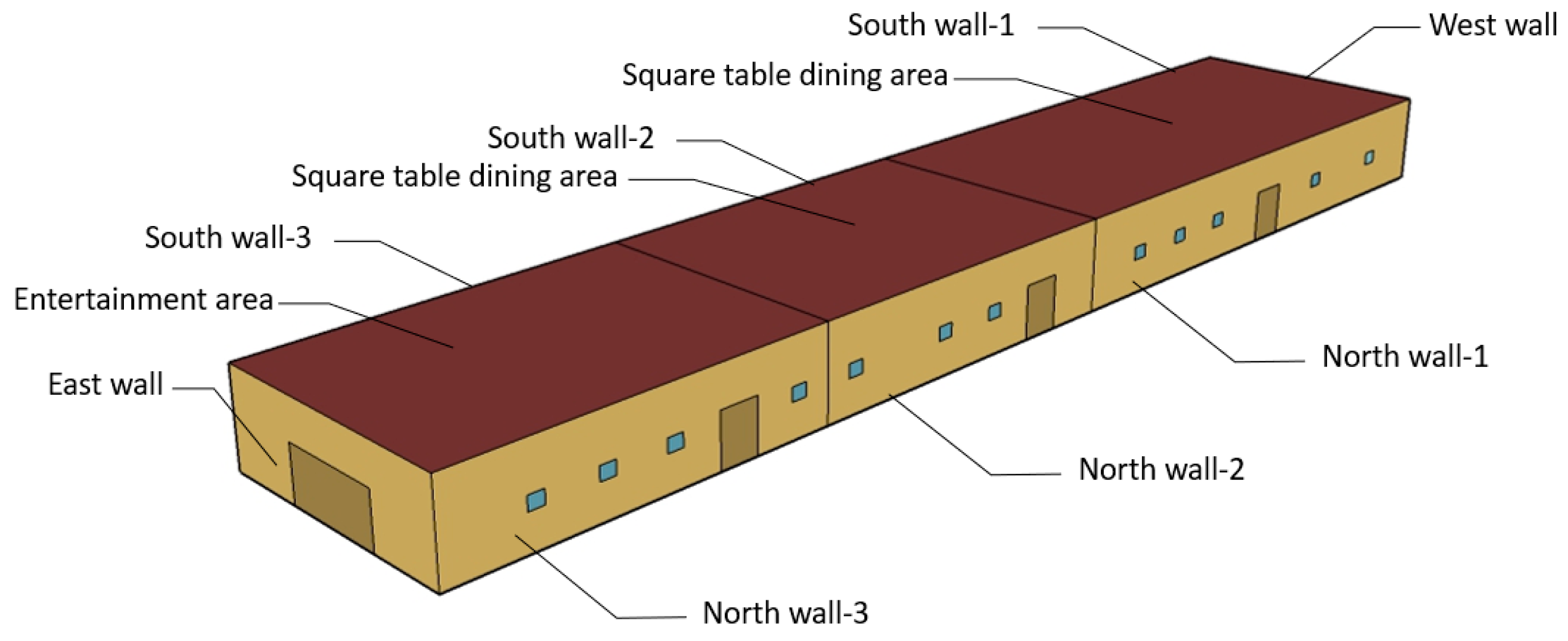
3.1. Physical Modeling of the Cruise Ship

The physical model presented herein is a restaurant and activity area of a medium-sized cruise ship, with dimensions of 50 m in length, 10 m in width, and 3.5 m in height. The cruise ship is present on the sea surface of Haikou, Hainan, and the local climate is tropical monsoon. The east, south, west, and north walls of the restaurant and activity area are located externally. The lower side of this area is the storage area of the cruise ship, and the upper side is the rest area for tourists, and both sides are air-conditioned. The cabin is divided into three areas according to the space function (Figure 2): from left to right, in the top view of the figure are Subzone I, Subzone II, and Subzone III. This area has 10 four-seater tables, five six-seater tables, and two round tables with 30 seats each. The assumption is that the occupancy is full for Subzone I and Subzone II, and the number of people in Subzone III changes according to different conditions. The maximum capacity in the entire space is 265 people. Additionally, according to the layout of HVAC terminals, 21 air supply outlets are arranged in the entire space.

3.2. EnergyPlus Modeling

To determine the temperature of the envelope inner surface and the air outlet supply air volume, the cabin was modeled using EnergyPlus, and the IDF file contained information about the building, internal load, and HVAC. The time chosen for the simulation was a typical summer day in Haikou, Hainan. Weather documents were provided by https://energyplus.net/ (accessed on 15 February 2023). Figure 3 shows a geometry model of the cabin modeled using EnergyPlus.

The detailed settings of the EnergyPlus model are summarized in

Table 2. Settings of the EnergyPlus model in the public space of the cruise ship.

Type	Subzone I	Subzone II	Subzone III
Dimension	22.05 m × 10 m	13.45 m × 10 m	14.5 m × 10 m
Occupants	70 × 100 W	60 × 100 W	n × 216 W
HVAC system	FCU	FCU	FCU
Ventilation system	0.00944 m3/s·per	0.00944 m3/s·per	0.00944 m3/s·per

. According to ASHRAE Standard 55–2020, the thermal power of a typical person is 100 W. The activity level in Subzone III was defined as light labor, and the thermal power was set to 216 W. This setting was consistent with the thermal boundary condition setting for personnel in Fluent. A typical summer day in Hainan was considered for the simulation, and the prediction of the inner surface temperature and air supply parameters of the envelope throughout the day was performed. The heat transfer coefficient of the exterior walls was 1.4 KW/(m²·K).

EnergyPlus modeling predicts the temperature of the inner surface wall of the cabin at different air-conditioning set temperatures, coupled with temperature setting in Fluent software, several times. In general, the average radiation temperature is highly representative of the indoor environment, but considering the inner wall temperature as one of the key points of data exchange in the coupling simulation, the inner wall temperature was selected for the reaction room environment [46]. Figure 4 shows the change pattern of the wall inner face temperature in Case 1. The temperature of the external walls gradually increased from 8:00 a.m. The temperature of the northern and southern walls began to decrease after reaching the peak value at 14:00. However, the temperature of the western wall continued to increase, reaching a peak of 29.43 °C at 18:00. Considering the overall variation, the load on the cabin peaked at 17:00. In the case of peak loads, coupled simulations of EnergyPlus and Fluent were performed. The inner surface temperature of walls and windows was set as boundary conditions for CFD simulation.

Through multiple coupled simulations of EnergyPlus and Fluent, the appropriate set temperature for the subzones was obtained (

Table 3. Control schemes for the indoor environment.

Case No.	Thermostats of Different Subzones (°C)
	Subzone I	Subzone II	Subzone III
1	27	27	24.5
2	27	26	24.5
3	27	26.5	24.5
4	27	26	25
5	27	26	25.5
6	27.5	26	26

). The thermostats of different subzones were used to control the supply air volumes of HVAC systems in the EnergyPlus simulation, which was also set for the boundary conditions of air outlets in the CFD simulation.

3.3. CFD Modeling

3.3.1. Meshing Scheme

Before performing CFD simulations, a suitable meshing scheme was identified to meet the governing equations that can be discrete into algebraic equations at each mesh point. The relationship between calculation time and accuracy was considered. Meshing with very low precision cannot yield accurate simulation results, whereas meshing with high precision can yield accurate results but requires extensive computer resources. After balancing accuracy and computer resources, the minimum grid unit was set as 0.05 m, and the grid size of the part that has only a slight effect on the result was appropriately relaxed to save computer resources. Finally, approximately 5 million hexahedral meshes were generated in the internal flow space of the studied space.

3.3.2. Numerical Process

To obtain the airflow patterns and temperature distributions of the indoor environment, the conservation equations of mass, momentum, and energy were considered. The general form of the governing equations was expressed as those in Equation (1), which includes four items: transient items, convective projects, diffusion projects, and source projects, expressed in formulas:

$$\frac{\partial \left(\rho \varphi \right)}{\partial t}+div\left(\rho \varphi \overrightarrow{u}\right)=div\left(\Gamma ·grad\varphi \right)+S_{\phi }$$

(1)

where $\phi$ is the dependent variable, which represents the velocity component $u_i$ in the $i$ dimension; $T$ is the temperature; $t$ is the time; $u$ is the velocity vector; $\Gamma$ is the diffusion coefficient; and $S_{\phi }$ is the source term.

Previous research results suggest that the k-ε model can be used to describe the characteristics of turbulent airflow in the indoor environment (

Table 4. Model settings for computational fluid dynamics simulation.

Name	Conditions
Models	Standard k-ε model
Methods	SIMPLE
Momentum	Second Order Upwind
Residual	continuity, momentum, turbulent flow energy, and turbulence dissipation rate are residuals < 1 × 10−3 energy < 1 × 10−6 (or the mass and energy errors of the entire system are less than 0.2%)

). Furthermore, the simulation results of the k-ε model were highly consistent with the experimental results. The standard k-ε model is the most widely used k-ε model, and its solution process is simpler than that of RNG and realizable turbulence models; hence, the standard k-ε model was selected in this research [33,47].

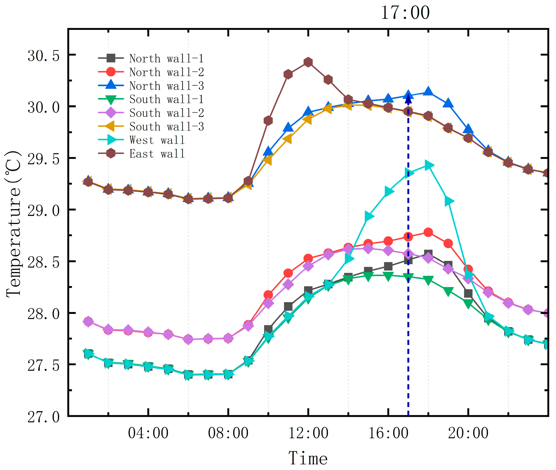
3.3.3. Boundary Conditions

For CFD simulation, boundary condition setting is a very important requirement apart from meshing. The model size and other conditions are consistent with those of EnergyPlus, and the human body model and objects in the research area are simplified. Precise boundary conditions in Fluent can be obtained based on outputs from EnergyPlus. Detailed settings of boundary conditions are shown in

Table 5. Detailed boundary condition settings.

Name	Case No.
	1	2	3	4	5	6
FCU-1 (each inlet) (m3/s)	0.104	0.117	0.118	0.117	0.118	0.119
FCU-2 (each inlet) (m3/s)	0.243	0.242	0.215	0.243	0.217	0.193
FCU-3 (each inlet) (m3/s)	0.042	0.091	0.128	0.151	0.179	0.2
Fresh air inlets (m3/s)	1.56	1.85	2.02	2.181	2.36	2.502
Occupants	0.5 m × 1.75 m × 1.3 m			Heat flux rate: 52.631 W/m2
(Double seating)
Occupants	0.5 m × 2.5 m × 1.3 m			Heat flux rate: 51.724 W/m2
(Three-seater)
Occupants	0.5 m × 9 m × 1.3 m			Heat flux rate: 51.370 W/m2
(Round-table seating)
Occupants	0.3 m × 0.5 m × 1.8 m			Heat flux rate: 71.260 W/m2
Entertainment)
Walls and Windows	Inside face temperature output from EnergyPlus

.

4. Results and Discussion

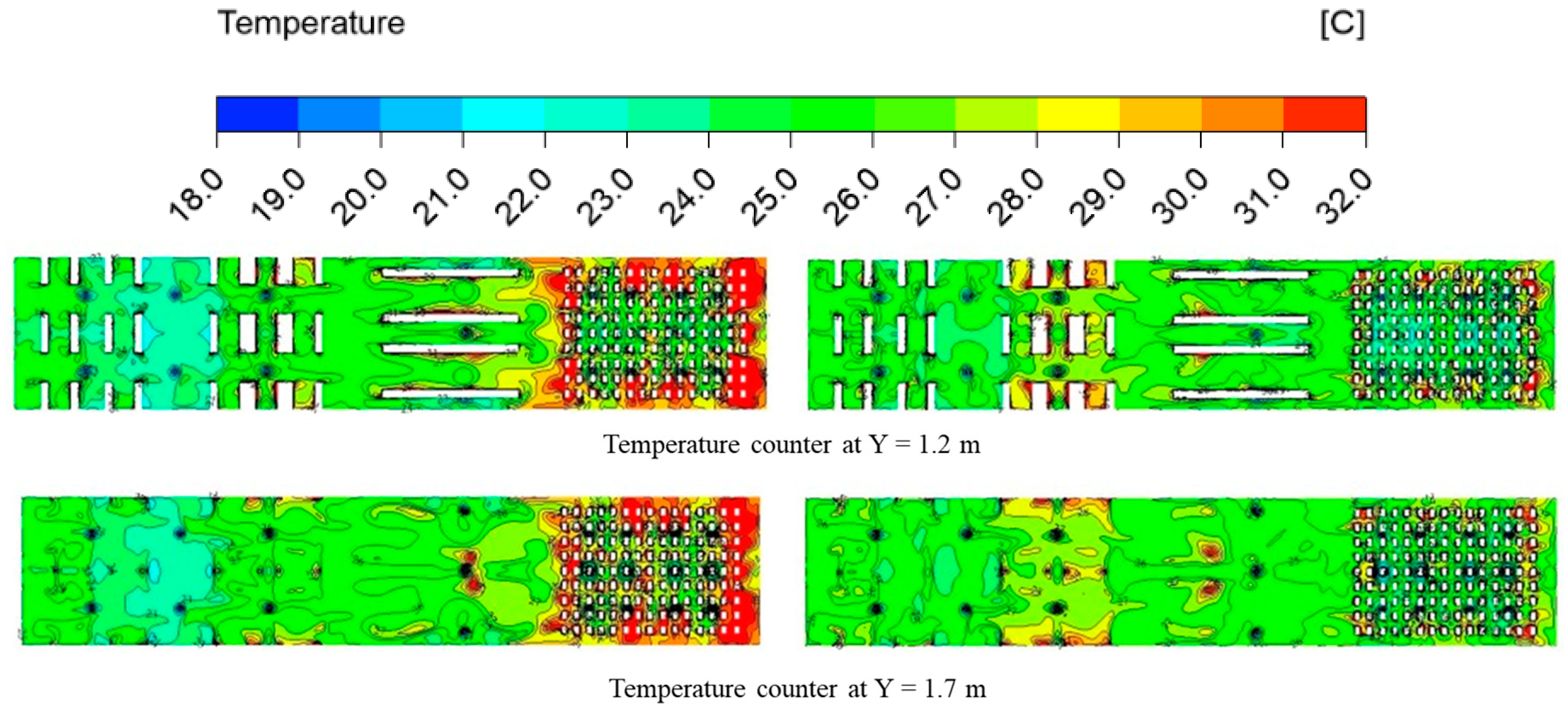
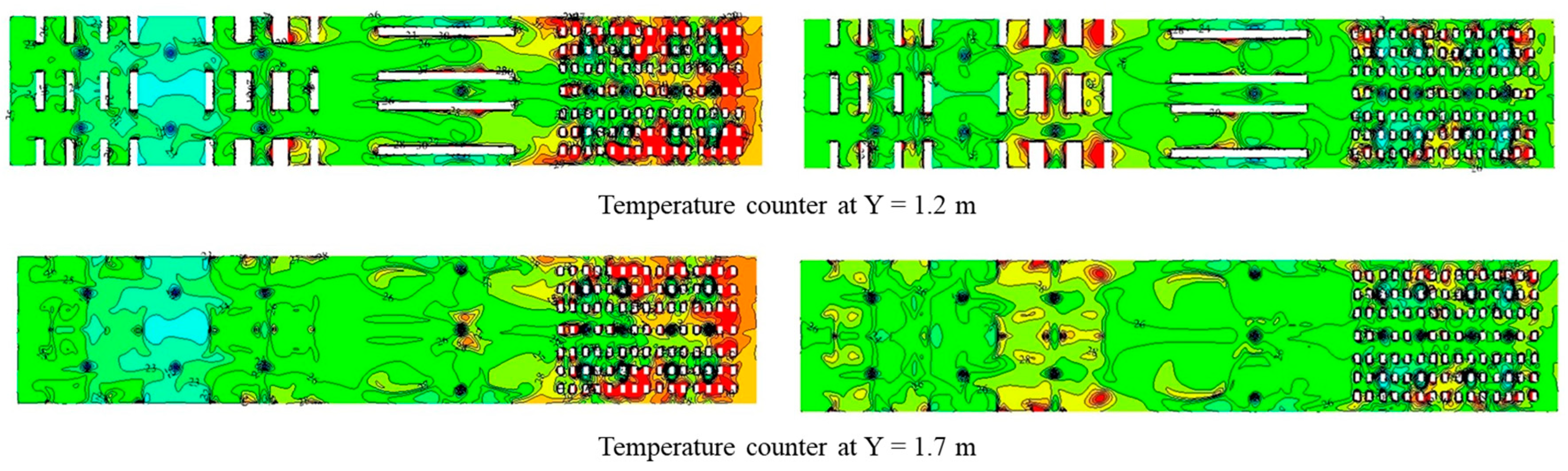
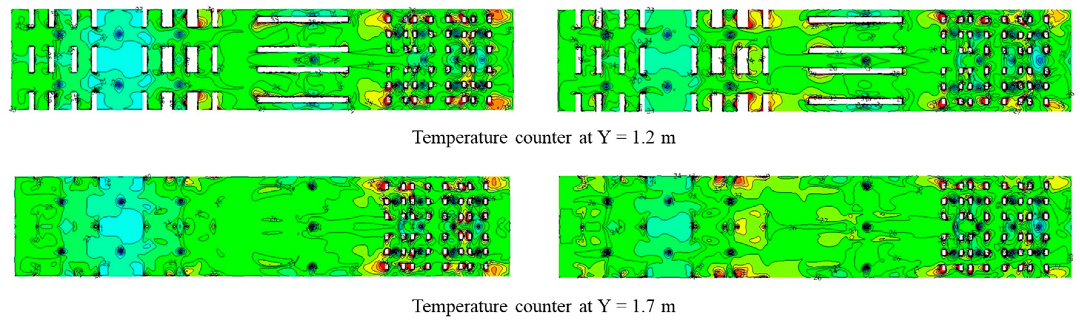
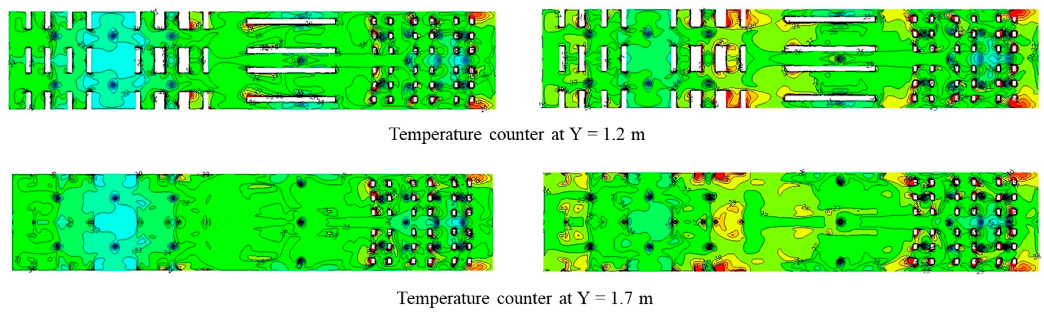
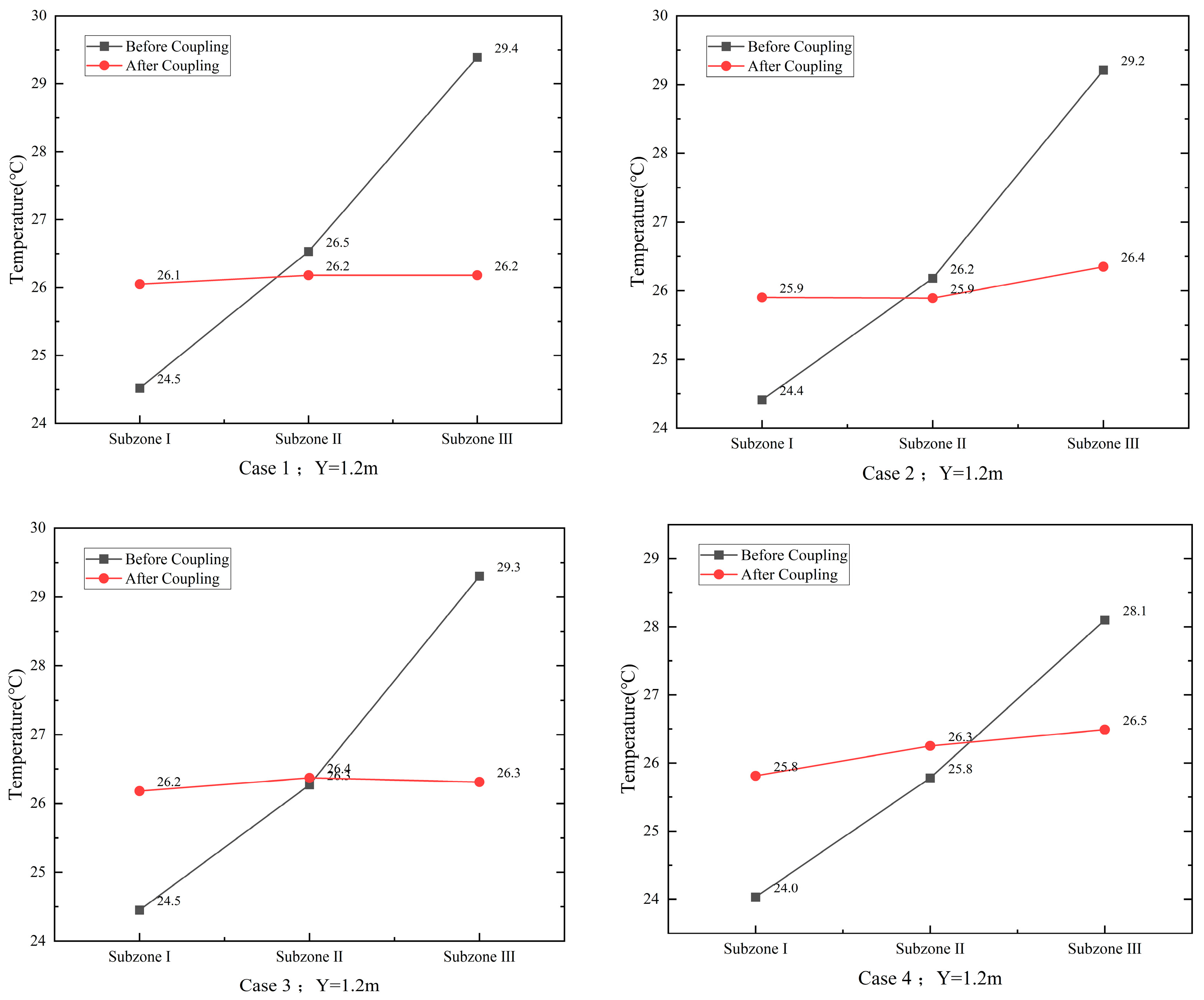
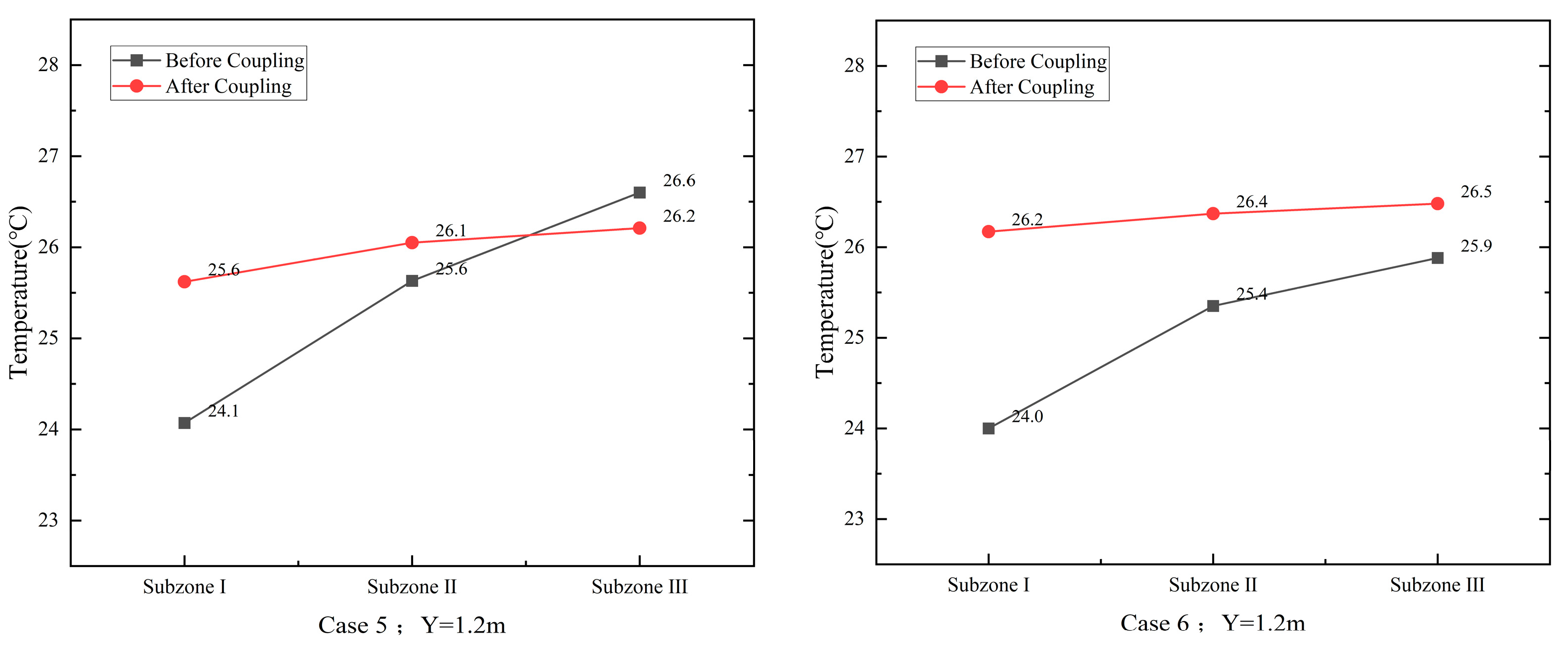
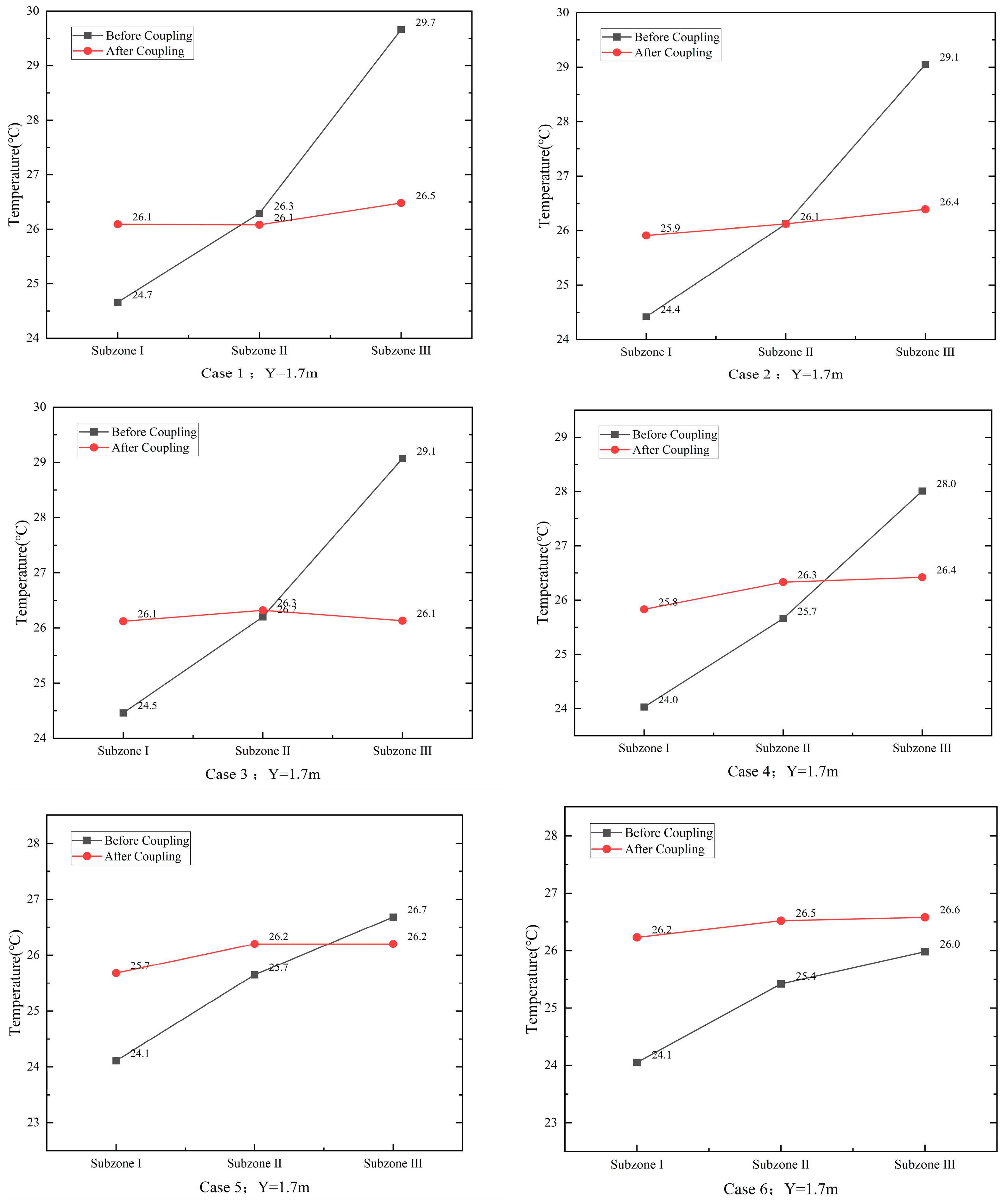
4.1. Temperature Comparison in the Subzones before and after Coupling Simulations

Using coupled simulations of EnergyPlus and Fluent, the temperature field of the public area was obtained. Two height levels were selected, namely Y = 1.2 m, i.e., the head level of the people seated, and Y = 1.7 m, i.e., the head level of the people standing. In Figure 5, Figure 6, Figure 7, Figure 8, Figure 9 and Figure 10, the figures on the left side illustrate temperature distributions under the unified temperature setting scheme. There are evident differences between the temperature setpoints and the simulated temperature. A significant uneven spatial temperature distribution was noted within the public space of the cruise ship. After several coupling comparisons, a suitable set temperature was obtained for the air conditioner in each zone. The figures on the right side of the images show the simulation results of the optimized zone temperature control scheme. The temperature distribution was relatively uniform, and the average temperature was close to the subzone temperature setpoints.

Combined with changes in the occupancy rate shown in Table 1 and the set temperature and temperature cloud of the air conditioner shown in Table 3, the decrease in the occupancy rate of Subzone III personnel had a direct effect on Subzone II and Subzone III, whereas that of Subzone I remained almost unaffected. Therefore, the temperature change of Subzone I was regarded as the change in the set temperature of the air conditioner under the change in the room rate of the overall personnel, and the temperature change of Subzone III was regarded as the change in the set temperature of the air conditioner under the change in the room rate of single area personnel. Therefore, the overall heat source in the room rate is reduced by 0.37, and the set temperature of the overall air conditioner needs to be increased by 0.5 °C. The occupancy rates of individual zones were reduced by 0.5 and 0.25, respectively, and the set temperature of the zone air conditioner increased by 0.5 °C.

Apart from the temperature fields, the average temperature of the three subzones under the single thermostat and subzone-based temperature setpoints was further compared. The average temperature deviation of different heights of six cases before and after optimization of subzone temperature control was analyzed. As shown in Figure 11 and Figure 12, when the unified temperature setpoint was 26 °C, the average temperature of the three subzones at Y = 1.2 m and 1.7 m was different from the set temperature. The maximum temperature difference occurred for Case 1 in Subzone III at Y = 1.7 m, where the average temperature was 3.7 °C higher than the temperature setpoint of 26 °C. The minimum temperature difference occurred for Case 6 in Subzone I at Y = 1.2 m, where the average temperature was 2 °C lower than the temperature setpoint, and the difference between the indoor demand temperature was 2 °C.

After zone control and optimization of the thermal environment, the average temperature for Case 6 in Subzone III at Y = 1.7 m was 26.6 °C, which differed only by 0.6 °C from the temperature setpoint. Considering all cases with variable occupancy rates in Subzone III, temperature differences between the average temperature of the three subzones and the subzone-based thermostat are within 1 °C, ranging from 0.4 °C to 0.7 °C. Therefore, this result indicates that the optimization method greatly improves the uniformity of regional temperature distribution.

4.2. Mass Exchange Rate between Subzones

As for the indoor environment, the air in the subzones is continuously exchanged for mass. However, EnergyPlus does not consider the change in energy consumption caused by this type of ass exchange when estimating energy consumption. Based on airflow patterns, the mass exchange law between the subzones is obtained using Fluent simulation. Figure 13 shows the mass exchange rate between subzones. For a positive value, the direction of mass exchange is the direction indicated in the legend. For a negative value, mass exchange is in the opposite direction shown in the legend. As the occupancy rate for Subzone III decreases, the direction of mass transfer changes. The transfer direction shifts between the occupancy rates of 0.5 and 0.6 for Subzone III. The change may have occurred because of the change in the occupancy rate, which may have caused a difference in the supply air volume and the temperature differences between subzones. From the perspective of the changing trend, the mass exchange rate between Subzone III and Subzone II is greater than that between Subzone II and Subzone I.

Figure 14 shows airspeed vectors in Subzone III after coupling BEM and CFD simulations. Based on the airflow patterns, the air supply volumes of the outlets decrease as the occupancy rate decreases. With the decrease in the occupancy rate, the disturbances from the occupants also weaken, resulting in more uniform distributions in air velocity. The amount of air entering Subzone III tends to increase gradually, leading to a change in the direction of mass exchange rates between adjacent subzones.

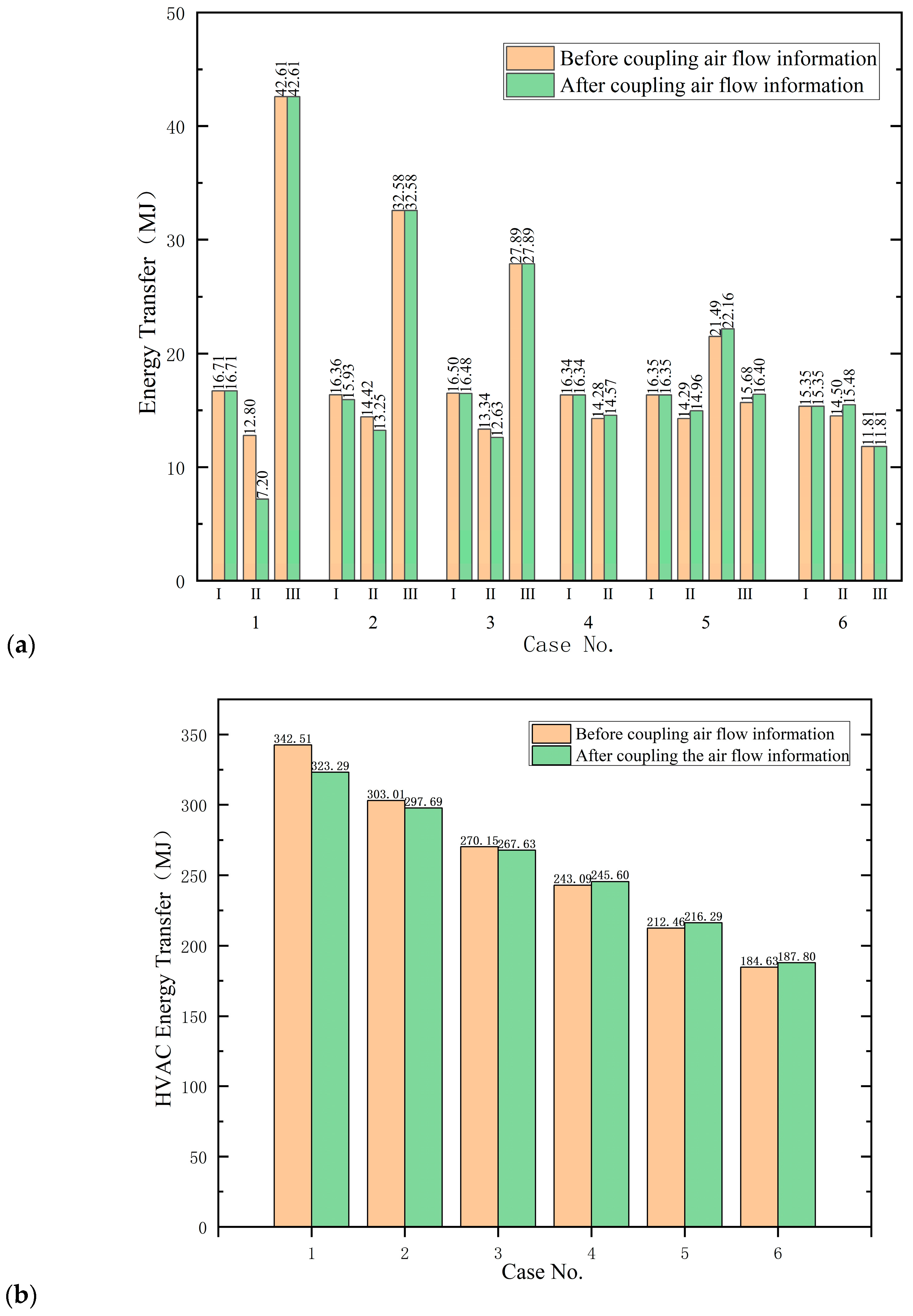
4.3. Analysis of Energy Consumption of HVAC Systems Considering Airflow Information

As the principle of EnergyPlus is based on the well-mixed model, this software application generally ignores airflow information for energy consumption analysis for well-mixed spaces. However, for large open spaces, the good-mixing assumption is not suitable because the temperature distribution is uneven. To explore the effect of mass exchange rates on energy consumption, the energy consumption with and without considering airflow information is compared. Figure 15 shows the estimation of energy consumption using EnergyPlus with and without considering mass exchange rates in six cases.

As shown in Figure 15, discrepancies exist in HVAC energy consumption with and without considering mass exchange rates between adjacent subzones. When Subzone III has a higher occupancy rate, the predicted energy consumption without considering the mass flow rate is higher than that with, considering the mass flow rate. When the occupancy rate is low, the energy consumption estimated using EnergyPlus without considering the mass flow rate is lower than that with considering the mass flow rate. Interestingly, after considering mass flow rates using EnergyPlus, the deviation in energy consumption at Subzone II is evident, whereas the deviation in energy consumption at Subzone I and Subzone III can be negligible.

Additionally, the temperature setpoint of Subzone I is the highest, followed by the temperature setpoints of Subzone II and Subzone III, respectively. The reason for the deviation in EnergyPlus in terms of the estimation of energy consumption may be that when Subzone III has a higher occupancy rate, the direction of mass transfer occurs from Subzone III to the other subzones at a relatively low temperature, which reduces the cooling load of Subzone I and Subzone II. When Subzone III has a lower occupancy rate, the direction of mass transfer occurs from Subzone I at a relatively high temperature to Subzone III at a low temperature setpoint, which may increase the cooling load of Subzone II and Subzone III.

Therefore, for large-space environments such as public spaces in a cruise ship, the results for energy consumption estimates are different regardless of whether the quality exchange of air is considered. It is considered that whether the energy consumption of air quality exchange is estimated to be greater than the original energy consumption estimate or less than the original energy consumption estimate is influenced by the direction of mass exchange. If the direction of mass exchange occurs from the low-temperature zone set by the air conditioner to the high-temperature zone, then the energy consumption of air quality exchange will be greater than the original energy consumption estimate; by contrast, if the exchange occurs from the high-temperature zone set by the air conditioner to the low-temperature zone, then the value will be smaller than the original energy consumption estimate.

4.4. Verification of the Accuracy of the Coupled Simulation

The accuracy of the coupled simulations in this study was evaluated by comparing the results of the first and second couplings. The first coupling refers to the coupling simulation results obtained after a suitable air-conditioning temperature and airflow control scheme has been determined. The second coupling refers to the transmission of the indoor air conditions obtained from the first coupling simulation to EnergyPlus by Fluent, which then outputs a second set of boundary conditions to Fluent for simulating the indoor thermal environment.

In the numerical simulation, the average temperatures of all areas at different heights were found to have slightly increased in the second coupling compared to the first coupling. The most significant change was observed in Subzone II, with an increase of 3.26% at Y = 2.5 m height, and an average increase of 3.10%. Subzone I increased by 1.64%, while Subzone III increased only by 0.088%. The temperature changes did not exceed 4%, indicating that the accuracy of the first coupling was higher than that of the second coupling.

In the energy consumption simulation, the inner wall temperatures were found to remain unchanged between the first and second couplings. Therefore, we can conclude that the accuracy of the coupled simulations is sufficient.

5. Discussion

As a solution to the problem of uneven distribution of thermal environment in large spaces, a zoning control method of air conditioning based on BEM-CFD coupling simulation has been proposed in this study, and an air-conditioning scheme has been established through multiple coupling simulations, which aids in optimizing the thermal environment of cruise public spaces. As for whether the energy consumption simulation results of mass exchange are considered, our results showed that, for a large-space environment, the size and direction of mass exchange affect energy consumption estimation. The present study concluded only the law of temperature setting of zonal air conditioners, and no quantitative algorithm has been established. In future research, factors such as personnel presence rate, partition area, and other factors should be considered, and a quantitative algorithm for temperature setting should be proposed to facilitate the determination of the air-conditioning zoning control temperature scheme. Based on the results of the coupling simulation, it is possible to build an automatic thermostat system for spaces with high comfort requirements. Thus, the technology of coupling simulation has become popular in production and daily life.

6. Conclusions

This study proposed coupling simulations of EnergyPlus and Fluent, a scheme used for optimizing the nonuniform thermal environment of a cruise ship. The subzone-based temperature setpoint approach can effectively optimize the thermal environment of a large open space. The appropriate temperature setpoints were determined by coupling simulations of BEM and CFD. The steady-state external bidirectional coupling method was adopted with parameter exchange. The relationship between the occupancy rate and the set temperature of the air conditioner was preliminarily discussed. EnergyPlus provides accurate boundary conditions required by Fluent, namely wall inner face temperature, window inner face temperature, and supply air volumes of air outlets. Through a feedback mechanism, Fluent enables temperature distributions and airflow patterns for EnergyPlus. Additionally, the influence of mass exchange rates on energy consumption was analyzed. When comparing the deviation of energy consumption estimation caused by the mass transmission of air, the law of energy consumption estimation in EnergyPlus was obtained. The main findings are as follows:

• Coupling simulation of EnergyPlus and Fluent can effectively solve the problem of uneven indoor temperature distribution in a large-space environment. By optimizing the indoor environment with the subzone-based temperature setpoint scheme, the temperature differences between the average temperature of the three subzones and the subzone-based thermostat range are within 1 °C, ranging from 0.4 °C to 0.7 °C.
• The temperature setting of the zone air conditioner is affected by two factors: the overall occupancy rate and the subzone occupancy rate. When the overall occupancy rate decreases by 0.37, the set temperature of the air conditioner in the large space increases by 0.5 °C. When the overall occupancy rate decreases by a certain value between 0.25 and 0.5, the set temperature of the air conditioner in the zone increases by 0.5 °C.
• With a decline in the occupancy rate of Subzone III, the direction of mass transmission from Subzone III to Subzone I changes to mass transmission from Subzone I to Subzone III. Changes occur when the occupancy rate of Subzone III is between 0.5 and 0.6. The change is possibly caused by the reduction in temperature differences between subzones and the decrease in supply air volumes in Subzone III, with declining occupancy rates.
• For large open spaces such as cruise public spaces, whether or not to consider the effects of zoning influences the size of the energy consumption simulation results. The direction of mass transfer and the temperature setpoint of the zone air conditioner, among other parameters, affect the simulation results.
• For the direction of mass transmission from the area with a low temperature setting value of the air conditioner to the area with a high-temperature set value, the energy consumption simulation result is less than the energy consumption simulation result without considering the mutual influence between partitions, and vice versa. To accurately reflect indoor energy consumption, the impact of the indoor environment on energy consumption should be considered in energy consumption simulations, and this rule may provide guidance for improving the accuracy of energy consumption estimates.

References

1. Cehlin, M.; Karimipanah, T.; Larsson, U.; Ameen, A. Comparing thermal comfort and air quality performance of two active chilled beam systems in an open-plan office. J. Build. Eng. 2019, 22, 56–65. [Google Scholar] [CrossRef]
2. Foucquier, A.; Robert, S.; Suard, F.; Stéphan, L.; Jay, A. State of the art in building modelling and energy performances prediction: A review. Renew. Sustain. Energy Rev. 2013, 23, 272–288. [Google Scholar] [CrossRef] [Green Version]
3. Pérez-Lombard, L.; Ortiz, J.; Pout, C. A review on buildings energy consumption information. Energy Build. 2008, 40, 394–398. [Google Scholar] [CrossRef]
4. Xie, D.; Li, K. Comprehensive Evaluation of Thermal Comfort in Ship Cabins: A Case Study of Ships in Yangtze River Basin, China. Buildings 2022, 12, 1766. [Google Scholar] [CrossRef]
5. Zhou, P.; Huang, G.; Zhang, L.; Tsang, K.-F. Wireless sensor network based monitoring system for a large-scale indoor space: Data process and supply air allocation optimization. Energy Build. 2015, 103, 365–374. [Google Scholar] [CrossRef]
6. Palella, B.I.; Quaranta, F.; Riccio, G. On the management and prevention of heat stress for crews onboard ships. Ocean Eng. 2016, 112, 277–286. [Google Scholar] [CrossRef]
7. Kong, M.; Zhang, J.; Wang, J. Air and air contaminant flows in office cubicles with and without personal ventilation: A CFD modeling and simulation study. Build. Simul. 2015, 8, 381–392. [Google Scholar] [CrossRef]
8. Oliveira, C.; Baptista, J.; Cerveira, A. Self-Sustainability Assessment for a High Building Based on Linear Programming and Computational Fluid Dynamics. Algorithms 2023, 16, 107. [Google Scholar] [CrossRef]
9. Si, C.; Qi, F.; Ding, X.; He, F.; Gao, Z.; Feng, Q.; Zheng, L. CFD Analysis of Solar Greenhouse Thermal and Humidity Environment Considering Soil–Crop–Back Wall Interactions. Energies 2023, 16, 2305. [Google Scholar] [CrossRef]
10. Sun, Z.; Wang, S. A CFD-based test method for control of indoor environment and space ventilation. Build. Environ. 2010, 45, 1441–1447. [Google Scholar] [CrossRef]
11. Chen, Q. Ventilation performance prediction for buildings: A method overview and recent applications. Build. Environ. 2009, 44, 848–858. [Google Scholar] [CrossRef]
12. Fletcher, C.A.J.; Mayer, I.F.; Eghlimi, A.; Wee, K.H.A. Cfd as a building services engineering tool. CANCES, University of New South Wales; CFD Research (S) Pte Ltd, Science Park II. Int. J. Archit. Sci. 2001, 2, 67–82. [Google Scholar]
13. Tsou, J. Strategy on applying computational fluid dynamic for building performance evaluation. Autom. Constr. 2001, 10, 327–335. [Google Scholar] [CrossRef]
14. Dahanayake, K.C.; Chow, C.L. Comparing reduction of building cooling load through green roofs and green walls by EnergyPlus simulations. Build. Simul. 2017, 11, 421–434. [Google Scholar] [CrossRef]
15. Alghoul, S.K. A Comparative Study of Energy Consumption for Residential HVAC Systems Using EnergyPlus. Am. J. Mech. Ind. Eng. 2017, 2, 98–103. [Google Scholar] [CrossRef] [Green Version]
16. Yu, T.; Heiselberg, P.; Lei, B.; Pomianowski, M. Validation and modification of modeling thermally activated building systems (TABS) using EnergyPlus. Build. Simul. 2014, 7, 615–627. [Google Scholar] [CrossRef]
17. Zhang, K.; Blum, D.; Cheng, H.; Paliaga, G.; Wetter, M.; Granderson, J. Estimating ASHRAE Guideline 36 energy savings for multi-zone variable air volume systems using Spawn of EnergyPlus. J. Build. Perform. Simul. 2022, 15, 215–236. [Google Scholar] [CrossRef]
18. Crawley, D.B.; Lawrie, L.K.; Pedersen, C.O.; Winkelmann, F.C. EnergyPlus: Energy simulation program. ASHRAE J. 2000, 42, 49–56. [Google Scholar]
19. Clarke, J.A. Energy simulation in building design: By J. A. Clarke; published by Adam Hilger Ltd, Techno House, Redcliffe Way, Bristol BS1 6NX, England; price: £36/$49; pp. 388; ISBN 0-85274-786-1, distributed in North America by Adam Hilger Ltd., P.O. Box 230, Accord, MA 02018, U.S.A., June 1985. Energy Build. 1986, 9, 263–266. [Google Scholar]
20. Clarke, J.A. The Implementation of a Computational Fluid Dynamics Algorithm within the ESP-r System; University of Strathclyde: Glasgow, Scotland, 2008. [Google Scholar]
21. Moser, A.; Off, F.; Schaelin, A.; Yuan, X. Numerical Modeling of Heat Transfer by Radiation and Convection in an Atrium with Thermal Inertia. In 36th Hemophilia Symposium Hamburg 2005; Springer: Berlin/Heidelberg, Germany, 2007. [Google Scholar]
22. Chen, Q.; Peng, X.; van Paassen, A.H.C. Prediction of Room Thermal Response by CFD Technique with Conjugate Heat Transfer and Radiation Models. In Proceedings of the 1995 ASHRAE Annual Meeting, San Diego, CA, USA, 24–28 June 1995; p. 11. [Google Scholar]
23. Mccormick, S.F. Multigrid Methods: Theory, Applications, and Supercomputing; CRC Press: Boca Raton, FL, USA, 1988; p. 2020. [Google Scholar]
24. Zhai, Z.; Chen, Q.; Haves, P.; Klems, J.H. On approaches to couple energy simulation and computational fluid dynamics programs. Build. Environ. 2002, 37, 857–864. [Google Scholar] [CrossRef]
25. Negrão, C.O.R. Integration of computational fluid dynamics with building thermal and mass flow simulation. Energy Build. 1998, 27, 155–165. [Google Scholar] [CrossRef]
26. Gijón-Rivera, M.; Xamán, J.; Álvarez, G.; Serrano-Arellano, J. Coupling CFD-BES Simulation of a glazed office with different types of windows in Mexico City. Build. Environ. 2013, 68, 22–34. [Google Scholar] [CrossRef]
27. Du, Z.; Xu, P.; Jin, X.; Liu, Q. Temperature sensor placement optimization for VAV control using CFD–BES co-simulation strategy. Build. Environ. 2015, 85, 104–113. [Google Scholar] [CrossRef]
28. Tian, W.; Zuo, W. Literature Review and Research Needs to Couple Building Energy and Airflow Simulation. In Proceedings of the APEC Conference on Low-Carbon Towns and Physical Energy Storage, Changsha, China, 25–26 May 2013. [Google Scholar]
29. Djunaedy, E.; Hensen, J.L.M.; Loomans, M.G.L.C. Toward External Coupling of Building Energy and Airflow Modeling Programs. ASHRAE Trans. 2003, 109, 771–787. [Google Scholar]
30. Manz, H.; Frank, T. Thermal simulation of buildings with double-skin facades. Energy Build. 2005, 37, 1114–1121. [Google Scholar] [CrossRef]
31. Hien, W.N.; Liping, W.; Chandra, A.N.; Pandey, A.R.; Xiaolin, W. Effects of double glazed facade on energy consumption, thermal comfort and condensation for a typical office building in Singapore. Energy Build. 2005, 37, 563–572. [Google Scholar] [CrossRef]
32. Yamamoto, T.; Ozaki, A.; Lee, M.; Kusumoto, H. Fundamental study of coupling methods between energy simulation and CFD. Energy Build. 2018, 159, 587–599. [Google Scholar] [CrossRef]
33. Barbason, M.; Reiter, S. Coupling building energy simulation and computational fluid dynamics: Application to a two-storey house in a temperate climate. Build. Environ. 2014, 75, 30–39. [Google Scholar] [CrossRef]
34. Zhang, R.; Mirzaei, P.A.; Jones, B. Development of a dynamic external CFD and BES coupling framework for application of urban neighbourhoods energy modelling. Build. Environ. 2018, 146, 37–49. [Google Scholar] [CrossRef]
35. Allegrini, J.; Carmeliet, J. Simulations of local heat islands in Zürich with coupled CFD and building energy models. Urban Clim. 2018, 24, 340–359. [Google Scholar] [CrossRef]
36. Ascione, F.; Bellia, L.; Capozzoli, A. A coupled numerical approach on museum air conditioning: Energy and fluid-dynamic analysis. Appl. Energy 2013, 103, 416–427. [Google Scholar] [CrossRef]
37. Tian, W.; Han, X.; Zuo, W.; Sohn, M.D. Building energy simulation coupled with CFD for indoor environment: A critical review and recent applications. Energy Build. 2018, 165, 184–199. [Google Scholar] [CrossRef]
38. Fan, Y.; Ito, K. Energy consumption analysis intended for real office space with energy recovery ventilator by integrating BES and CFD approaches. Build. Environ. 2012, 52, 57–67. [Google Scholar] [CrossRef]
39. Shan, X.; Luo, N.; Sun, K.; Hong, T.; Lee, Y.-K.; Lu, W.-Z. Coupling CFD and building energy modelling to optimize the operation of a large open office space for occupant comfort. Sustain. Cities Soc. 2020, 60, 102257. [Google Scholar] [CrossRef]
40. Zhang, R.; Mirzaei, P.A.; Jones, B.M. Dynamic simulation of cross-ventilated buildings with night-flush cooling in neighbourhood environment using integrated CFD-CFD-BES strategy. IOP Conf. Ser. Mater. Sci. Eng. 2019, 609, 072023. [Google Scholar] [CrossRef]
41. Zhang, R.; Mirzaei, P.A. Fast and dynamic neighbourhood energy simulation using CFDf-CFDc-BES coupling method. Sustain. Cities Soc. 2020, 66, 102545. [Google Scholar] [CrossRef]
42. Fabrizio, A.; Francesca, D.M.R.; Margherita, M.; Peter, V.G. The design of safe classrooms of educational buildings for facing contagions and transmission of diseases: A novel approach combining audits, calibrated energy models, building performance (BPS) and computational fluid dynamic (CFD) simulations. Energy Build. 2021, 230, 110533. [Google Scholar]
43. Martin, P. CFD in the real world: HVAC&R applications; software and hardware; creating a CFD model; reducing project costs. ASHRAE J. 1999, 41, 20. [Google Scholar]
44. Djunaedy, E. Selecting an appropriate tool for airflow simulation in buildings. Build. Serv. Eng. Res. Technol. 2004, 25, 269–278. [Google Scholar] [CrossRef]
45. Djunaedy, E.; Hensen, J.L.M.; Loomans, M.G.L.C. External Coupling between CFD and Energy Simulation: Implementation and Validation. ASHRAE Trans. 2005, 111, 612–624. [Google Scholar]
46. D’Ambrosio Alfano, F.R.; Olesen, B.W.; Pepe, D.; Palella, B.I. Working with Different Building Energy Performance Tools: From Input Data to Energy and Indoor Temperature Predictions. Energies 2023, 16, 743. [Google Scholar] [CrossRef]
47. Rohdin, P.; Moshfegh, B. Numerical predictions of indoor climate in large industrial premises. A comparison between different k-ε models supported by field measurements. Build. Environ. 2007, 42, 3872–3882. [Google Scholar] [CrossRef]
Figure 1. Framework of the building energy modeling–computational fluid dynamics coupling simulation.
Energies 16 03214 g001
Figure 2. Layout of the public space of the cruise ship from (a) top view and (b) three-dimensional view.
Energies 16 03214 g002
Figure 3. Geometric model of the cabin modeled using EnergyPlus.
Energies 16 03214 g003
Figure 4. Change patterns of the wall inner face temperature.
Energies 16 03214 g004
Figure 5. Temperature fields before and after coupling in Case 1.
Energies 16 03214 g005
Figure 6. Temperature fields before and after coupling in Case 2.
Energies 16 03214 g006
Figure 7. Temperature fields before and after coupling in Case 3.
Energies 16 03214 g007
Figure 8. Temperature fields before and after coupling simulations in Case 4.
Energies 16 03214 g008
Figure 9. Temperature fields before and after coupling simulations in Case 5.
Energies 16 03214 g009
Figure 10. Temperature fields before and after coupling simulations in Case 6.
Energies 16 03214 g010
Figure 11. Comparison of the average temperature under different thermostat schemes at Y = 1.2 m.
Energies 16 03214 g011aEnergies 16 03214 g011b
Figure 12. Comparison of the average temperature under different thermostat schemes at Y = 1.7 m.
Energies 16 03214 g012
Figure 13. Mass flow exchange rates between adjacent subzones.
Energies 16 03214 g013
Figure 14. Airspeed vectors after coupling simulations in Subzone III at the middle plane of Z = 5 m.
Energies 16 03214 g014
Figure 15. Comparison of energy consumption with and without considering airflow information. (a) Comparison of energy transfer in subzones; (b) Comparison of energy transfer in heating, ventilating, and air-conditioning systems. I: Subzone I; II: Subzone II; III: Subzone III.
Energies 16 03214 g015