Integrated Energy Microgrid Economic Dispatch Optimization Model Based on Information-Gap Decision Theory

Abstract

To address the problems of “difficult to consume” renewable energy and the randomness of power output, we propose the CHP unit joint-operation model with power to gas (P2G) and carbon capture system (CCS) technologies and analyze the operation cost, carbon emission, and “electric-heat coupling” characteristics of this model. A dispatch optimization model is constructed based on the information-gap decision theory under the strategy to further consider the interval uncertainty of renewable energy unit output and load forecast. The optimized-dispatching model effectively solves the fate of renewable unit output and electric-thermal load and provides dispatching strategies for decision-makers to balance risk and capital management.

1. Introduction

In recent years, the environmental pollution problems caused by carbon emissions [1] have become increasingly severe, forcing human society to gradually transition to a renewable energy-based [2], green, low-carbon, and sustainable energy [3] era. Promoting low-carbon development [4] has called for global consensus, and China has put forward the goal of achieving carbon peaking by 2030 and carbon neutrality by 2060. The energy sector [5] accounts for a large share of total carbon emissions. The energy sector needs to be decarbonized by following both low-carbon policy and technology paths [6]. Two typical examples are using renewable energy to generate electricity [7] and carbon capture (CCS) [8] to reduce carbon emissions. According to the National Energy Administration (NEA) [9], China’s installed wind power and photovoltaic (P.V.) capacities reached 198 million kW and 190 million kW, respectively, in 2022; however, energy abandonment remains prominent due to the intermittent and fluctuating nature of new energy generation. The literature [10] points out that, as of 2017, the amount of abandoned wind and P.V. in China was as high as 41.9 billion kW·h and 7.3 billion kW·h, respectively. An integrated energy microgrid [11] is a management tool that can integrate renewable energy and demand-side load resources, becoming the smallest power supply unit closest to the customer. In actual operation, renewable energy consumption and carbon emission reduction are limited due to the cost of the energy storage configuration [12] and its anti-peaking characteristics [13].

From the perspective of an integrated energy dispatching strategy [14,15,16], most existing studies focus on the economic dispatching of integrated energy systems. Zhao et al. [17] proposed a decoupling solution method for the optimal energy flow of electricity, heat and gas from multiple energy sources, which could determine the system operation when the cost is optimal by introducing multi-intelligent bodies for collaborative optimization of each energy source. Dong et al. [18] proposed the establishment of a multi-objective energy-saving dispatching model containing the production, environmental and coordination costs of cooling, heating and electricity. Mohammad et al. [19] proposed an IES economic dispatch model that considers the uncertainty of wind and light output and the uncertainty of electric and thermal loads by considering the fate of supply and demand. Gerda et al. [20] considered the relevance of the interaction between electricity, natural gas and thermal systems in an integrated energy system. A regional joint environmental and economic dispatch model for combined cooling, heating, and power (CCHP) systems under peak and valley tariffs was designed to minimize the transaction cost of power purchase and sale plans, fuel and environmental costs from the emission of harmful gases. All of the above studies considered the influence of uncertainty on the supply side and load side to varying degrees, focusing on the optimal economic dispatch of IES, and establishing an economic dispatch model to use to solve a determined equipment dispatch strategy, but did not discuss in depth the environmental aspects of IES. Liu et al. [21] proposed a grid economic dispatch model considering the prediction error under high renewable energy penetration. Although the increased penetration of renewable energy was considered, the economy was still the main optimization objective.

In the study of uncertainty problems, stochastic [22] and robust [23] optimization are mainstream; the idea is generally to perform information representation of uncertain quantities based on probabilistic scenarios or hesitant sets and further obtain the planning costs. For example, Peng et al. [24] constructed a microgrid source-load-storage optimal scheduling model based on the predicted power values of wind, P.V. and load, which is essentially deterministic scheduling due to using power prediction curves to characterize the uncertain variables. The results were affected by the prediction errors. Liu et al. [25], using the Latin hypercube sampling method to sample uncertainties, generated typical representative scenarios using the simultaneous back-generation reduction technique to construct deterministic energy dispatch models. For the generation of tentative plans, probability curves of tensions are required. Still, typical systems may have errors due to the imprecise construction of the probability distribution models. Many scenarios reduce the computational efficiency, and the reduction of methods also makes the model lose its robustness. Ding et al. [26] constructed a robust optimization-based economic optimal dispatch model for microgrids. Complete optimization describes uncertain variables by creating uncertainty sets. It calculates the optimal solution of the objective function in the worst case. The configuration scheme was too conservative because the economics of the decision was sacrificed to improve the robustness of the decision. The information-gap decision theory [27,28,29] can quantify uncertainty and solve the decision scheme flexibly by seeking the uncertainty set of the maximum acceptable fluctuation range of uncertain parameters in the optimization process based on specific expected objectives with less information about the amount of uncertainty. Compared with robust optimization, the information-gap decision theory model does not require a given fluctuation range of tension and can find the optimal solution on a limited budget. At present, IGDT has been applied to wind power-dispatching decisions [30], the strategy of power purchasing and selling companies under multiple retail contract models [31], and medium- and long-term operation risk measurement under multiple markets of graded hydropower [32]. However, there are fewer studies on applying IGDT models to integrated energy microgrids for day-ahead dispatching.

In this paper, we consider the uncertainty of demand response and scenic power output to build an economic dispatch model of an integrated energy microgrid with carbon capture and electricity-to-gas synergies to reduce the amount of wind and CO₂ emissions from the integrated energy microgrid and realize the reasonable control and utilization of the uncertainty of renewable energy power output by managers.

2. Integrated Energy Microgrid System Architecture

The structure of the integrated energy microgrid system based on renewable generating units, P2G equipment, carbon-capture equipment, CHP units, and demand-response integration is shown in Figure 1. The microgrid service provider intelligently dispatches in response to customers’ electricity demands and unifies each unit’s generation plan to balance supply and demand.

Power side: The energy consumption of CCS and P2G units is provided by CHP units and wind and P.V. units. CCS provides the CO₂ consumed by P2G units.

Customer side: By implementing the peak-to-peak tariff, customers are guided to respond to the system dispatch with the scenery output curve to reduce the electrical load during load supply and demand tension.

2.1. Combined-Operation Mode of CHP Units with P2G and CCS

In this paper, P2G technology is introduced to CHP units together with CCS technology. During low electricity-load demand, CHP units use P2G technology to convert surplus renewable energy into recyclable natural gas resources and increase renewable energy consumption. For the system’s carbon emissions, the CCS unit can capture the CO₂ emitted from the flue gas tail of the CHP unit, and the captured CO₂ can be transported to the P2G unit to produce renewable resources, such as methane, reducing the carbon purchase cost of the P2G unit while increasing the operating profit of the CHP unit. In the following paper, we explain the operation principle of the combined-operating mode of the CHP unit with CCS and P2G technology in terms of its operation characteristics, CO₂ emission characteristics, system operation cost, and constraints.

2.1.1. Characterization of the Combined-Operation Mode of CHP Units with CCS and P2G Technologies

The output power of the CHP unit in the combined-operation mode of CHP with CCS and P2G technologies is composed of the operating capability of the P2G unit, the operational capacity of the CCS unit, and the actual grid power of the CHP unit, respectively, as shown in Equation (1).

$$P_{\mathrm{CHP},t}=P_{\mathrm{CHP},\mathrm{E},t}+P_{\mathrm{P}2\mathrm{G},t}+P_{\mathrm{CCS},t}$$

(1)

The range of CHP unit output in the combined-operation mode of CHP with CCS and P2G technology is shown in Equation (2).

$$P_{\mathrm{CHP},\min }\le P_{\mathrm{CHP},l}\le P_{\mathrm{CHP},\max }$$

(2)

The power constraint of the P2G device is shown in Equation (3).

$$P_{\mathrm{P}2\mathrm{G},\min }\le P_{\mathrm{P}2\mathrm{G},l}\le P_{\mathrm{P}2\mathrm{G},\max }$$

(3)

where $P_{\mathrm{P}2\mathrm{G},\min }$ and $P_{\mathrm{P}2\mathrm{G},\max }$ are the minimum and maximum values of the operating power consumption of the P2G device, respectively.

The CCS unit operates in the absorption, resolution, and compression of CO₂ with the electrical power constraint shown in Equation (4).

$$P_{\mathrm{CCS},\min }\le P_{\mathrm{CCS},t}\le P_{\mathrm{CCS},\max }$$

(4)

where $P_{\mathrm{CCS},\min }$ and $P_{\mathrm{CCS},\max }$ are the minimum and maximum values of the operating consumption of the CCS unit, respectively.

The CHP unit’s thermal power output range in CHP’s combined-operation mode with CCS and P2G technology is shown in Equation (5).

$$H_{\mathrm{CHP},\min }\le H_{\mathrm{CHP},t}\le H_{\mathrm{CHP},\max }$$

(5)

where $H_{\mathrm{CHP},\min }$ and $H_{\mathrm{CHP},\max }$ are the minimum and maximum values of the thermal power of the CHP unit under the combined-operation mode of CHP with CCS and P2G technologies, respectively.

Finally, the electric-thermal coupling characteristics of the CHP unit in the combined-operation mode of CHP with CCS and P2G technology are shown in Equation (6).

$$\begin{array}{l}\max \left\{P_{\mathrm{CHP},\mathrm{E},\min }-c_{\mathrm{v}1}{H}_{\mathrm{CHP},l},c_m\left(H_{\mathrm{CHP},l}-H_{\mathrm{CHP},\min }\right)-P_{\mathrm{PZG},\max }\right.\\ \left.-P_{\mathrm{CCS},\max }\right\}\le P_{\mathrm{CHP},\mathrm{E},t}\le P_{\mathrm{CHP},\mathrm{E},\max }-c_{v_2}{H}_{\mathrm{CHP},t}-P_{\mathrm{PQG},\min }-P_{\mathrm{CCS},\min }\end{array}$$

(6)

This paper utilizes a pumped CHP unit because the system operation characteristics, as depicted in Figure 2, can control the unit within a specific range of output of electric and thermal power. The explicit adjustable content is shown in the envelope ACEF in Figure 2. The two lines, AC and FE, indicate the CHP unit’s maximum and minimum output electric power. AF shows the current system operation under the pure condensing condition. Currently, AF offers the current system operation under pristine condensing conditions. At this point, the unit enters pure power generation mode; so, it can be seen in Figure 2 that the system is not outputting thermal power under the current operating condition. The two points of AF represent this CHP unit’s maximum and minimum electric power output values under the current functional state. When the CHP unit operates in CE, most of the steam extracted from the intermediate turbine stage is used for thermal power output, where the maximum power output point is C. The system can reduce the CHP unit’s electric power output when operating in CE line mode. The thermal result of the system in the intermediate state is indicated, and the regulation range of the electric power output of the CHP unit is BD, as can be seen in Figure 2.

In the combined-operation mode of CHP with CCS and P2G technology, the electric-thermal output range of CHP units is the ACGHI region in Figure 2. The combined-operation mode of CHP with CCS and P2G technology increases the flexible space of the CHP unit, and the CHP unit with P2G and CCS can provide a smaller actual system output at a particular heat output.

The range constraint of the P2G output gas power is shown in Equation (7).

$$G_{\mathrm{P}2\mathrm{G},\min }=\frac{P_{\mathrm{P}2\mathrm{G},\min }}{\alpha }\le G_{\mathrm{P}2\mathrm{G},t}\le \frac{P_{\mathrm{P}2\mathrm{G},\max }}{\alpha }=G_{\mathrm{P}2\mathrm{G},\max }$$

(7)

where $G_{\mathrm{P}2\mathrm{G},t}$ is the output gas power of the P2G device at time t, and $G_{\mathrm{P}2\mathrm{G},\max }$, $G_{\mathrm{P}2\mathrm{G},\min }$ are the maximum and minimum values of the gas transmission power, respectively.

In the combined-operating mode of the CHP unit with CCS and P2G technology, the flexible space of the CHP unit is increased, and it is more adaptable to participate in microgrid dispatch optimization. The gas power output of the P2G unit is maximum when $P_{\mathrm{CHP},\mathrm{E},t}=P_{\mathrm{CHP},\mathrm{E},\min }-c_{v1}{H}_{\mathrm{CHP},t}$ and $P_{\mathrm{CHP},\mathrm{E},t}=c_m\left(H_{\mathrm{CHP},t}-H_{\mathrm{CHP},\min }\right)-P_{\mathrm{P}2\mathrm{G},\max }-P_{\mathrm{CCS},\max }$ when $P_{\mathrm{CHP},\mathrm{E},t}=P_{\mathrm{CHP},\mathrm{E},\max }-c_{\mathrm{Vl}}{H}_{\mathrm{CHP},t}$ the P2G output gas power is minimum.

In the combined-operation mode of CHP units accounting for CCS and P2G technologies, the gas power constraint of the CHP units accounting for CCS and P2G technologies is shown in Equation (8).

$$\begin{array}{l}\max \left\{\frac{\alpha }{1-\xi \beta }\left[\left(P_{\mathrm{CHP},\min }-c_{\mathrm{v}1}{H}_{\mathrm{CHP},t}\right),c_m\left(H_{\mathrm{CHP},t}-H_{\mathrm{CHP},\min }\right)-P_{\mathrm{CHP},\mathrm{E},t}\right]\right\}\le \\ G_{\mathrm{P}2\mathrm{G},t}\le \frac{\alpha }{1-\xi \beta }\left(P_{\mathrm{CHP},\max }-c_{\mathrm{v}2}{H}_{\mathrm{CHP},t}-P_{\mathrm{CHP},\mathrm{E},t}\right)\end{array}$$

(8)

Therefore, the CHP unit with CCS and P2G technologies in combined-operation mode realizes the multi-energy complementarity of electricity, gas, and heat. The CHP units with P2G technology can convert excess electricity into natural gas when the electrical load is low, which improves the operating efficiency of CHP units and enhances the consumption of renewable energy at the same time.

2.1.2. Calculation of Carbon Emission of CHP Unit Combined-Operation Mode with CCS and P2G Technology

As the most widely used thermal power generation unit, the pumped CHP unit generates a large amount of CO₂ during stable operation, and the amount of CO₂ generated is shown in Equation (9).

$$Z_{\mathrm{CHP},t}=a_{{\mathrm{co}}_2}\left(P_{\mathrm{CHP},t}+c_{\mathrm{v}1}{H}_{\mathrm{CHP},t}\right)+b_{{\mathrm{co}}_2}{\left(P_{\mathrm{CHP},t}+c_{\mathrm{vl}1}{H}_{\mathrm{CHP},t}\right)}^2+c_{{\mathrm{co}}_2}$$

(9)

where $Z_{\mathrm{CHP},t}$ is the CHP unit emissions of CO₂ at time t, $a_{{\mathrm{co}}_2}$, $b_{{\mathrm{co}}_2}$,$c_{{\mathrm{co}}_2}$ are the carbon emission factors of the coal unit.

When a CHP unit with a CCS unit is in stable operation, part of the CO₂ generated will be captured by the CCS unit, so the actual carbon emissions from the CHP unit are shown in Equation (10).

$$Z_{\mathrm{CCP},t}=a_{{\mathrm{co}}_2}\left(P_{\mathrm{CHP},t}+c_{v1}{H}_{\mathrm{CHP},t}\right)+b_{{\cos }_2}{\left(P_{\mathrm{CHP},t}+c_{\mathrm{v}1}{H}_{\mathrm{CHP},t}\right)}^2+c_{{\mathrm{co}}_2}-Z_{\mathrm{CCS},t}$$

(10)

where $Z_{\mathrm{CCP},t}$ gives the CHP unit emissions of CO₂ with the CCS device at time t.

2.1.3. The Operating Cost of CHP Unit Combined-Operation Mode with CCS and P2G Technology

Under the combined-operating mode of the CHP unit with CCS and P2G technology, the CHP unit’s operating costs consist of the CHP unit’s generation cost, the CCS unit’s operating cost, and the operating cost of the P2G unit. Since the power consumed by the P2G and CCS units comes from the CHP unit, the energy cost of the P2G and CCS units is unified in the power generation cost of the CHP unit.

(1)

P2G unit-operating costs

The operating cost of a P2G unit is mainly composed of the cost of using the P2G unit and the cost of purchasing carbon, as shown in Equation (11).

$$C_{\mathrm{P}2\mathrm{G}}={\displaystyle \sum _{t=1}^T{c}_{\mathrm{P}2\mathrm{G}}}{P}_{\mathrm{P}2\mathrm{G},t}+d_{\mathrm{P}2\mathrm{G}}{Z}_{\mathrm{P}2\mathrm{G},t}$$

(11)

where $C_{\mathrm{P}2\mathrm{G}}$ is the operating cost of the P2G unit, $c_{\mathrm{P}2\mathrm{G}}$ is the usage cost factor of the P2G unit, $d_{\mathrm{P}2\mathrm{G}}$ is the purchased carbon cost factor of the P2G unit, and $Z_{\mathrm{P}2\mathrm{G},t}$ is the amount of carbon consumed by the operation of the P2G unit at time t.

(2)

CCS unit operating costs

The CCS unit operating cost is mainly related to the CCS unit operating loss cost, as shown in Equation (12).

$$C_{\mathrm{CCS}}={\displaystyle \sum _{t=1}^T{c}_{\mathrm{CCS}}}{P}_{\mathrm{CCS},t}$$

(12)

where $C_{\mathrm{CCS}}$ is the operating cost of the CCS unit, and $c_{\mathrm{CCS}}$ is the functional loss factor of the CCS unit.

(3)

CO₂ storage costs

The CCS unit captures and stores the CO₂ emitted from the CHP unit. The amount of CO₂ stored in the system is the difference between the amount of CO₂ charged by the CCS unit and the amount of CO₂ consumed by the P2G unit. This is shown in Equation (13).

$$C_{\mathrm{FC}}={\displaystyle \sum _{t=1}^T{c}_{\mathrm{E}}}\left(Z_{\mathrm{CHP},t}-Z_{\mathrm{P}2\mathrm{G},t}\right)$$

(13)

where $c_{\mathrm{E}}$ is the carbon sequestration cost factor.

(4)

Combined-operating costs of CHP units with P2G and CCS technologies are taken into account

The total system operating cost $C_{\mathrm{CCP}}$ for the combined-operation mode of CHP units with P2G and CCS technologies is:

$$C_{\mathrm{CCP}}=C_{\mathrm{CHP}}+C_{\mathrm{P}2\mathrm{G}}+C_{\mathrm{CCS}}+C_{\mathrm{FC}}$$

(14)

2.1.4. Combined-Operation Constraints of CHP Units Taking into Account P2G and CCS Technologies

The CHP unit constraints in the combined-operation mode of CHP with P2G and CCS technologies mainly include the output limit constraint, CHP unit ramp-up constraint, and CCS carbon-capture operation constraint.

(1)

Climbing constraint of CHP units with P2G and CCS technologies

The climbing constraint of the CHP unit in CCP combined-operation mode is shown in Equation (15).

$$\Delta P_{\mathrm{CCP},\min }\le \left(P_{\mathrm{CHP},\mathrm{E},t}+P_{\mathrm{pQG},t}+P_{\mathrm{CCS},t}\right)-\left(P_{\mathrm{CHP},\mathrm{E},t-1}+P_{\mathrm{PQC},t-1}+P_{\mathrm{CCS},t-1}\right)\le \Delta P_{\mathrm{CCP},\max }$$

(15)

where $\Delta P_{\mathrm{CCP},\max }$ and $\Delta P_{\mathrm{CCP},\min }$ are the maximum and minimum values of the climbing rate of CHP unit under the CCP combined-operation mode, respectively.

(2)

CCS carbon-capture operational constraints

The CCS carbon-capture-range constraint is shown in Equation (16).

$$\begin{array}{l}{Z}_{\mathrm{CCS},t}\le a_{{\mathrm{coo}}_2}\left(P_{\mathrm{CHP},\mathrm{E},t}+P_{{\mathrm{PQ}}_2,t}+P_{\mathrm{CCS},t}+c_{\mathrm{v}l}{H}_{\mathrm{CHP},}\right)\\ +b_{{\mathrm{co}}_2}{\left(P_{\mathrm{CHP},\mathrm{E},t}+P_{{\mathrm{PVG}}_{2\mathrm{G}},t}+P_{\mathrm{CCS},t}+c_{{\mathrm{vl}}^2}{H}_{\mathrm{CHP},t}\right)}^2+c_{{\mathrm{co}}_2}\end{array}$$

(16)

2.2. Demand-Response Model

2.2.1. Analysis of the Principle of Time-Sharing Tariffs

According to customer-side electricity consumption habits, daily electricity consumption is usually divided into three periods: peak–valley–even. The price elasticity of the demand matrix of electricity generally refers to the ratio of the change in demand for electricity triggered by the amount of difference in electricity price on a particular day, as shown in Equation (17).

$$E=\left[\begin{array}{cccc}{E}_{11}& E_{12}& \dots & E_{1n}\\ E_{21}& E_{22}& \dots & E_{2n}\\ E_{31}& E_{32}& \ddots & ⋮\\ E_{41}& \dots & \dots & E_{nn}\end{array}\right]$$

(17)

where n represents the period when the electricity price increases at a specific time, the customer can reduce the electricity demand or shift the electricity load to other periods, then, the self-elasticity factor is negative, and the cross-elasticity factor is positive.

Based on the price elasticity of the demand matrix to model the peak–valley time-sharing tariff, the amount of change in electricity consumption on the customer side is

$$\left[\begin{array}{c}\Delta D_{1,t}/D_{1,t}^{\mathrm{imt}}\\ \Delta D_{2,t}/D_{2,t}^{\mathrm{imt}}\\ ⋮\\ \Delta D_{n,t}/D_{n,t}^{\mathrm{inn}}\end{array}\right]=\frac{1}{n}E\left[\begin{array}{c}\Delta {\rho }_{1,t}/{\rho }_{1,t}^{\mathrm{int}}\\ \Delta {\rho }_{2,t}/{\rho }_{2,t}^{\mathrm{int}}\\ ⋮\\ \Delta {\rho }_{n,t}/{\rho }_{n,t}^{\mathrm{imt}}\end{array}\right]$$

(18)

This yields the customer’s electricity consumption under demand response as:

$$\left[\begin{array}{c}{D}_{1,t}^{\prime }\\ D_{2,t}^{\prime }\\ ⋮\\ D_{n,t}^{\prime }\end{array}\right]=\frac{1}{n}\left[\begin{array}{llll}{D}_{1,t}\hfill & \hfill & \hfill & \hfill \\ \hfill & D_{2,t}\hfill & \hfill & \hfill \\ \hfill & \hfill & \ddots \hfill & \hfill \\ \hfill & \hfill & \hfill & D_{n,t}\hfill \end{array}\right]E\left[\begin{array}{c}\Delta {\rho }_{1,t}/{\rho }_{1,t}^{\mathrm{int} }\\ \Delta {\rho }_{2,t}/{\rho }_{2,t}^{\mathrm{int} }\\ ⋮\\ \Delta {\rho }_{n,t}/{\rho }_{n,t}^{\mathrm{int} }\end{array}\right]+\left[\begin{array}{c}{D}_{1,t}\\ D_{2,t}\\ ⋮\\ D_{n,t}\end{array}\right]$$

(19)

where $D_{n,t}^{\prime }$ is the customer’s electricity consumption at n moments under demand response.

2.2.2. Demand-Response Cost Model

The price elasticity of demand refers to the sensitivity of customer load to electricity price, including the self-elasticity and cross-elasticity factors. The impact of the electricity price on the current load is the self-elasticity factor. In contrast, the effect of electricity price at that moment on the bag at other moments is the cross-elasticity factor.

$$E_{t,t}^j=\frac{{\rho }_{j,l}^{\mathrm{int}}\Delta D_{j,l}}{D_{j,t}^{\mathrm{int}}\Delta {\rho }_{j,t}}$$

(20)

$$E_{t,h}^j=\frac{{\rho }_{j,h}^{\mathrm{int}}\Delta D_{j,t}}{D_{j,t}^{\mathrm{int}}\Delta {\rho }_{j,h}}$$

(21)

where ${\rho }_{j,l}^{\mathrm{int}}$ and ${\rho }_{j,h}^{\mathrm{int}}$ are the initial electricity price of user j at moments t and h, respectively; $\Delta {\rho }_{j,t}$ and $\Delta {\rho }_{j,h}$ are the price change to user j at moments t and h, respectively; $\Delta D_{j,l}$ denote the amount of load change to user j under demand response.

$$D_{j,t}^{\mathrm{int}}=D_{j,t}^{\mathrm{end}}+\Delta D_{j,t}$$

(22)

Under the price demand response mechanism, the customer’s electricity load changes from $D_{j,t}^{\mathrm{int}}$ to $D_{j,t}^{\mathrm{end}}$. The benefits to the microgrid operator on the customer side j are

$$S\left(D_{j,t}^{\mathrm{end} }\right)=B\left(D_{j,l}^{\mathrm{end} }\right)-D_{j,l}^{\mathrm{end} }{\rho }_{j,l}$$

(23)

where $B\left(D_{j,l}^{\mathrm{end} }\right)$ is the microgrid operator the profit gain under the price demand-response mechanism; $D_{j,l}^{\mathrm{end} }{\rho }_{j,l}$ is the compensation cost of the microgrid operator to the customers.

When the transferable load and the curtailable load jointly participate in the demand response, the amount of freight for users within the microgrid to respond to the demand-response mechanism is

$$D_{j,t}^{end}=(1-\lambda )D_{j,t}^{\mathrm{int}}+{\lambda }_j\left[{\displaystyle \sum _{\begin{array}{c}t=1\\ t\ne h\end{array}}^T{D}_{j,t}^{\mathrm{int}}}{E}_{t,h}^j\frac{{\rho }_{j,h}-{\rho }_{j,h}^{\mathrm{int}}}{{\rho }_{j,h}^{\mathrm{int}}}+D_{j,t}^{\mathrm{int}}\right]$$

(24)

where ${\lambda }_j$ is the weight in response to the demand-response mechanism.

3. Deterministic Integrated Energy Microgrid Optimal Economic Dispatch Model

This paper aims at the lowest total operating cost for integrated energy microgrid energy management. The entire operating cost C of the microgrid comprises the CHP unit operating cost ${\mathrm{C}}_{\mathrm{t}}^{\mathrm{CHP}}$, energy storage plant system operating cost ${\mathrm{C}}_{\mathrm{t}}^{\mathrm{ESS}}$, external interaction cost ${\mathrm{C}}_{\mathrm{t}}^{\mathrm{utility} }$, carbon trading cost ${\mathrm{C}}_{\mathrm{t}}^{{\mathrm{CO}}_2}$, gas boiler operating cost $C_{\mathrm{GB}}$, and demand-response cost ${\mathrm{C}}_{\mathrm{t}}^{\mathrm{DR}}$, by taking into account P2G and CCS technologies.

3.1. Integrated Energy Microgrid Operating Costs

(1)

CHP unit operating cost

The operating cost ${\mathrm{C}}_{\mathrm{t}}^{\mathrm{CHP}}$ of the CHP unit, taking into account CCS and P2G technologies, is

$$C_{\mathrm{CCP}}=C_{\mathrm{CHP}}+C_{\mathrm{P}2\mathrm{G}}+C_{\mathrm{CCS}}+C_{\mathrm{FC}}$$

(25)

(2)

External interaction costs

Microgrid external interaction costs ${\mathrm{C}}_{\mathrm{t}}^{\mathrm{utility} }$ include the energy purchase and sale costs resulting from interaction with the parent grid or gas network.

$${\mathrm{C}}_{\mathrm{t}}^{\mathrm{utility} }={\displaystyle \sum _{\mathrm{t}}^{\mathrm{T}}\left[\left(\mathrm{U}{\mathrm{p}}_{\mathrm{k},\mathrm{t}}^{{\mathrm{CH}}_4}{\mathrm{V}}_{\mathrm{k},\mathrm{t}}^{\mathrm{buy} }\right)+\left(\mathrm{U}{\mathrm{p}}_{\mathrm{t}}^{\mathrm{buy} }{\mathrm{P}}_{\mathrm{k},\mathrm{t}}^{\mathrm{buy} }-\mathrm{U}{\mathrm{p}}_{\mathrm{t}}^{\mathrm{sell} }{\mathrm{P}}_{\mathrm{k},t}^{\mathrm{sell} }\right)\right]}$$

(26)

where $\mathrm{U}{\mathrm{p}}_{\mathrm{k},\mathrm{t}}^{{\mathrm{CH}}_4}$ is the unit price per unit of natural gas purchased; ${\mathrm{V}}_{\mathrm{k},\mathrm{t}}^{\mathrm{buy} }$ is the amount of gas purchased when the CHP system is in operation; and $\mathrm{U}{\mathrm{p}}_{\mathrm{t}}^{\mathrm{buy} }$, $\mathrm{U}{\mathrm{p}}_{\mathrm{t}}^{\mathrm{sell} }$ is the unit price of electricity bought and sold, respectively.

(3)

Energy storage system operating costs

The operating cost of ESS ${\mathrm{C}}_{\mathrm{t}}^{\mathrm{ESS}}$ is

$${\mathrm{C}}_{\mathrm{t}}^{\mathrm{ESS} }={\displaystyle \sum _{\mathrm{t}}^{\mathrm{T}}\zeta }\left({\mathrm{P}}_{\mathrm{k},\mathrm{t}}^{\mathrm{ESSinput} }+{\mathrm{P}}_{\mathrm{k},\mathrm{t}}^{\mathrm{ESSouput} }\right)$$

(27)

where $\zeta$ is the cost factor of energy storage system operation.

(4)

Carbon quota and carbon trading costs

$$C_{{\mathrm{co}}_2}={\displaystyle \sum _{t=1}^T\epsilon }\left(E_t-E_{0,t}\right)$$

(28)

(5)

Demand-response cost

Transferring or disconnecting the load requires compensation from the customer.

$${\mathrm{C}}_{\mathrm{t}}^{\mathrm{DR}}={\displaystyle \sum _{\mathrm{t}}^{\mathrm{T}}\left({\mathsf{\lambda }}_{\mathrm{e}}^{\mathrm{cut}}{\mathrm{P}}_{\mathrm{k},\mathrm{t}}^{\mathrm{cut}}+{\mathsf{\lambda }}_{\mathrm{e}}^{\mathrm{tran}}{\mathrm{P}}_{\mathrm{k},\mathrm{t}}^{\mathrm{tran}}+{\mathsf{\lambda }}_{\mathrm{h}}^{\mathrm{cut}}{\mathrm{H}}_{\mathrm{k},\mathrm{t}}^{\mathrm{cut}}\right)}$$

(29)

where ${\mathrm{C}}_{\mathrm{t}}^{\mathrm{DR}}$ is the demand-response and compensation costs for load shifting and load shedding, respectively.

(6)

Gas boiler operating costs

The operating cost of the gas turbine $C_{\mathrm{GB}}$ is

$$C_{\mathrm{GB}}={\displaystyle \sum _{t=1}^T{a}_{\mathrm{GB}}}{G}_{\mathrm{MT},t}$$

(30)

In summary, the minimum operating costs of an integrated energy microgrid are

$$\min (C)=C_{\mathrm{CCP}}+{\mathrm{C}}_{\mathrm{t}}^{\mathrm{ESS}}+C_{{\mathrm{co}}_2}+C_{\mathrm{GB}}+{\mathrm{C}}_{\mathrm{t}}^{\mathrm{utility} }+{\mathrm{C}}_{\mathrm{t}}^{\mathrm{DR}}$$

(31)

where C is the total operating cost of the integrated energy microgrid day-ahead dispatch model.

3.2. Constraints

Integrated energy microgrid management needs to meet the electricity–gas–power balance constraint and ensure that each unit output constraint is as follows.

(1)

Electrical power balance

The electrical power balance constraint of the integrated energy system microgrid management is shown in Equation (32).

$$P_{\mathrm{Wind},t}+P_{\mathrm{PV},t}+P_{\mathrm{CHP},\mathrm{E},t}+P_{\mathrm{BS},\mathrm{disch},t}+P_{k,t}^{\mathrm{buy} }=P_{\mathrm{Load},t}+P_{\mathrm{BS},\mathrm{ch},t}+P_{k,t}^{\mathrm{sell} }$$

(32)

where $P_{\mathrm{Load},I}$ is the electrical load of the integrated energy system at time t.

(2)

Thermal power balance

The thermal power balance constraint for integrated energy microgrid management is shown in Equation (33).

$$H_{\mathrm{CHP},t}+H_{\mathrm{GB},t}=H_{\mathrm{Load},t}$$

(33)

where $H_{\mathrm{Load},t}$ is the thermal load of the integrated energy microgrid at time t.

(3)

G.B. unit operating constraints

The G.B. unit output power and the climbing slope constraint are represented by Equations (34) and (35),

$$H_{\mathrm{GB},\min }\le H_{\mathrm{GB},t}\le H_{\mathrm{GB},\max }$$

(34)

$$\Delta H_{\mathrm{GB},\min }\le H_{\mathrm{GB},t}-H_{\mathrm{GB},t-1}\le \Delta H_{\mathrm{GB},\max }$$

(35)

where $H_{\mathrm{GB},\min }$ and $H_{\mathrm{GB},\max }$ are the upper and lower limits of the gas turbine output power and the minimum and maximum values of the gas turbine output climbing slope, respectively.

(4)

Electricity sales constraints

The integrated energy microgrid power sales constraint is shown in Equation (36).

$$P_{\mathrm{sell},\min }<P_{\mathrm{sell},I}<P_{\mathrm{sell},\max }$$

(36)

where $P_{\mathrm{sell},\min }$ and $P_{\mathrm{sell},\max }$ are the upper and lower limits of the sold power.

(5)

Gas purchase constraints

The integrated energy microgrid purchased gas power constraint is shown in Equation (37).

$$G_{S,\min }\le G_{S,t}\le G_{S,\max }$$

(37)

where $G_{S,\min }$ and $G_{S,\max }$ are the upper and lower limits of purchased gas power, respectively.

(6)

Gas power balance constraint

The gas balance constraint satisfied by the integrated energy microgrid in day-ahead dispatch optimization is shown in Equation (38).

$$G_{\mathrm{P}2\mathrm{G},t}+G_{S,t}=G_{\mathrm{GB},t}$$

(38)

where $G_{S,t}$ is the purchased gas power of the integrated energy microgrid at time t.

4. Interval Uncertainty and IGDT Optimization Model

4.1. Interval Uncertainty Model

This paper uses envelope constraints to describe the uncertainty of wind power, P.V. output, and electric and thermal loads. The interval uncertainty model for renewable energy is as follows:

$$U\left({\alpha }_{\mathrm{s}},{\tilde{P}}_t^{\mathrm{S}}\right)=\left\{P_t^{\mathrm{S}}:\left|P_t^{\mathrm{S}}-{\tilde{P}}_t^{\mathrm{S}}\right|\le {\alpha }_{\mathrm{S}}{\tilde{P}}_t^{\mathrm{s}}\right\}$$

(39)

$$U\left({\alpha }_{\mathrm{w}},{\tilde{P}}_t^{\mathrm{w}}\right)=\left\{P_t^{\mathrm{w}}:\left|P_t^{\mathrm{w}}-{\tilde{P}}_t^{\mathrm{w}}\right|\le {\alpha }_{\mathrm{w}}{\tilde{P}}_t^{\mathrm{w}}\right\}$$

(40)

$$U\left({\alpha }_H,{\tilde{L}}_{h,t}\right)=\left\{L_{h,t}:\left|L_{h,t}-{\tilde{L}}_{h,t}\right|\le {\alpha }_H{\tilde{L}}_{h,t}\right\}$$

(41)

$$U\left({\alpha }_E,{\tilde{L}}_{\mathrm{e},t}\right)=\left\{L_{\mathrm{e},t}:\left|L_{\mathrm{e},t}-{\tilde{L}}_{\mathrm{e},t}\right|\le {\alpha }_E{\tilde{L}}_{\mathrm{e},t}\right\}$$

(42)

where ${\tilde{P}}_t^{\mathrm{s}}$, ${\tilde{P}}_t^{\mathrm{w}}$, ${\tilde{L}}_{h,t}$ and ${\tilde{L}}_{\mathrm{e},t}$ are the predicted values of P.V. output, wind-power output, and thermal-power load demand at time t, respectively; ${\alpha }_{\mathrm{S}}$, ${\alpha }_{\mathrm{w}}$, ${\alpha }_H$ and ${\alpha }_E$ are the uncertainties of wind-power output, wind-power output, and thermal-power load demand, respectively.

The conventional IGDT is only applicable to deal with a single uncertainty quantity. This phase combines the three tensions using a weighted sum to determine the system’s combined uncertainty to account for the uncertainty of the environment and load concurrently.

$$\psi ={\lambda }_{\mathrm{S}}{\alpha }_{\mathrm{S}}+{\lambda }_{\mathrm{W}}{\alpha }_{\mathrm{W}}+{\lambda }_H{\alpha }_H+{\lambda }_E{\alpha }_E$$

(43)

where $\psi$ is the integrated uncertainty of the microgrid energy management system; ${\lambda }_{\mathrm{S}}$, ${\lambda }_{\mathrm{W}}$, ${\lambda }_H$ and ${\lambda }_E$ are the weighting coefficients of the fate of P.V. output, wind-power output, and thermal-electricity demand, respectively, reflecting the degree of need from the decision makers for the system to cope with scenery as well as load uncertainty, independent of the model itself.

4.2. IGDT Optimization Model

For the risk preferences of different microgrid operators, the integrated energy microgrid scheduling optimization models under risk-averse strategy and opportunity seeking are given in this paper based on IGDT, under the satisfaction of expected cost deviation.

4.2.1. Risk Avoidance Strategy

The risk-averse strategy maximizes the uncertainty of the uncertainty quantity while ensuring that the optimization objective is within the acceptable range of the decision-maker. Specifically, the economic-scheduling problem studied in this paper is to maximize the integrated uncertainty of the system. In contrast, the scheduling cost of the system does not exceed the expected price. The larger the uncertainty value, the more risk-averse the approach is and the more robust the scheduling scheme.

Therefore, the objective function of the risk-averse IGDT scheduling model is shown in Equation (45). s.t. Equations (1)–(43) and (45)–(49).

$$Max{\psi }_{\mathrm{r}}$$

(44)

$$Max{C}_g+C_{qt}\le (1+{\beta }^{RM})C_g$$

(45)

$$P_t^{\mathrm{S}}\in U\left({\alpha }_{\mathrm{s}},{\tilde{P}}_t^{\mathrm{S}}\right)$$

(46)

$$P_t^{\mathrm{w}}\in U\left({\alpha }_{\mathrm{w}},{\tilde{P}}_t^{\mathrm{w}}\right)$$

(47)

$$L_{h,t}\in U\left({\alpha }_H,{\tilde{L}}_{h,t}\right)$$

(48)

$$L_{\mathrm{e},t}\in U\left({\alpha }_E,{\tilde{L}}_{\mathrm{e},t}\right)$$

(49)

where $C_g$ is the dispatch cost’s baseline value, obtained by bringing the predicted values of wind, photovoltaic and electric-thermal loads into the deterministic dispatch model for optimization; ${\beta }^{RM}$ is the robustness level factor, which reflects the dispatcher’s ability to accept additional costs.

It can be seen that the above IGDT scheduling model is a two-layer optimization model. The lower layer indicates that the system dispatch cost cannot exceed the expected price when the photovoltaic output, wind-power output, and electric-thermal load demands fluctuate within the uncertainty set. Therefore, the robust optimization model in this paper can be transformed into a single-layer optimization model objective function as in Equation (45)

$$P_t^{\mathrm{S}}=(1-{\alpha }_{\mathrm{s}}){\tilde{P}}_t^{\mathrm{S}}$$

(50)

$$P_t^{\mathrm{w}}=(1-{\alpha }_{\mathrm{w}}){\tilde{P}}_t^{\mathrm{w}}$$

(51)

$$L_{h,t}=(1+{\alpha }_H){\tilde{L}}_{h,t}$$

(52)

$$L_{\mathrm{e},t}=(1+{\alpha }_E){\tilde{L}}_{\mathrm{e},t}$$

(53)

s.t. Equations (1)–(43), (46)–(49) and (55).

4.2.2. IGDT Opportunity Optimization Model for Risk Appetite

For the optimal operation of the microgrid, the problem studied in this paper, i.e., to minimize the integrated uncertainty of the microgrid when the operating cost of the microgrid does not exceed the expected operating price; the more significant, the lower the probability of achieving the desired operating cost of the microgrid; however, the less sensitive the operating strategy is to the fluctuation of the uncertainty quantity, the safer the microgrid.

Therefore, the objective function of this paper’s risk-averse IGDT optimization model is shown in Equation (56).

$$Min{\psi }_o$$

(54)

$$Min{C}_g+C_{qt}\le (1-{\beta }^{RM})C_g$$

(55)

s.t. Equations (1)–(43), (46)–(49) and (55).

Similarly, the opportunity optimization model is transformed into a single-layer optimization model with the objective function as in Equation (56).

$$P_t^{\mathrm{S}}=(1+{\alpha }_{\mathrm{s}}){\tilde{P}}_t^{\mathrm{S}}$$

(56)

$$P_t^{\mathrm{w}}=(1+{\alpha }_{\mathrm{w}}){\tilde{P}}_t^{\mathrm{w}}$$

(57)

$$L_{h,t}=(1-{\alpha }_H){\tilde{L}}_{h,t}$$

(58)

$$L_{\mathrm{e},t}=(1-{\alpha }_E){\tilde{L}}_{\mathrm{e},t}$$

(59)

s.t. Equations (1)–(43), (55) and (56)–(59).

4.3. Optimization Model Solving

4.3.1. IGDT Model-Solving Method

The information-gap decision theory model established in this chapter is a two-layer optimization model with complex solutions. The objective of the lower layer of the robust model is the lowest operating cost of the integrated energy microgrid. In this paper, we used the toolbox YALMIP in MATLAB to build an integrated energy microgrid economic optimization model and used the GUROBI solver to solve it.

4.3.2. IGDT Model Solving Steps

① The predicted output value of light and wind turbines $\left({\tilde{P}}_t^{\mathrm{S}},{\tilde{P}}_t^{\mathrm{w}}\right)$ and the predicted demand value of heat and power $\left({\tilde{L}}_{h,t},{\tilde{L}}_{\mathrm{e},t}\right)$ are brought into the deterministic microgrid optimization model. The optimal value of the microgrid operation cost $C_0$ is found and called the base value of the IGDT model.

② Substitution of the actual values of the light–wind unit output $\left(P_t^{\mathrm{S}},P_t^{\mathrm{w}}\right)$ and the actual values of the thermal-electric load demand $\left(L_{h,t},L_{\mathrm{e},t}\right)$ for the forecasted values is made, and then the development of the cost deviation factors ${\beta }^{RM}$, the desired target values of the robust optimization model $\left(1+{\beta }^{RM}\right)C_0$ acceptable to the scheduler and the desired target values of the opportunity optimization model $\left(1-{\beta }^{RM}\right)C_0$;

③ The IGDT opportunity optimization model under the risk-preference strategy and IGDT robust optimization model under the risk-averse strategy is solved to obtain the integrated uncertainty, scheduling cost and day-ahead scheduling strategy.

The flowchart for solving the IGDT scheduling model is shown in Figure 3.

5. Example Analysis

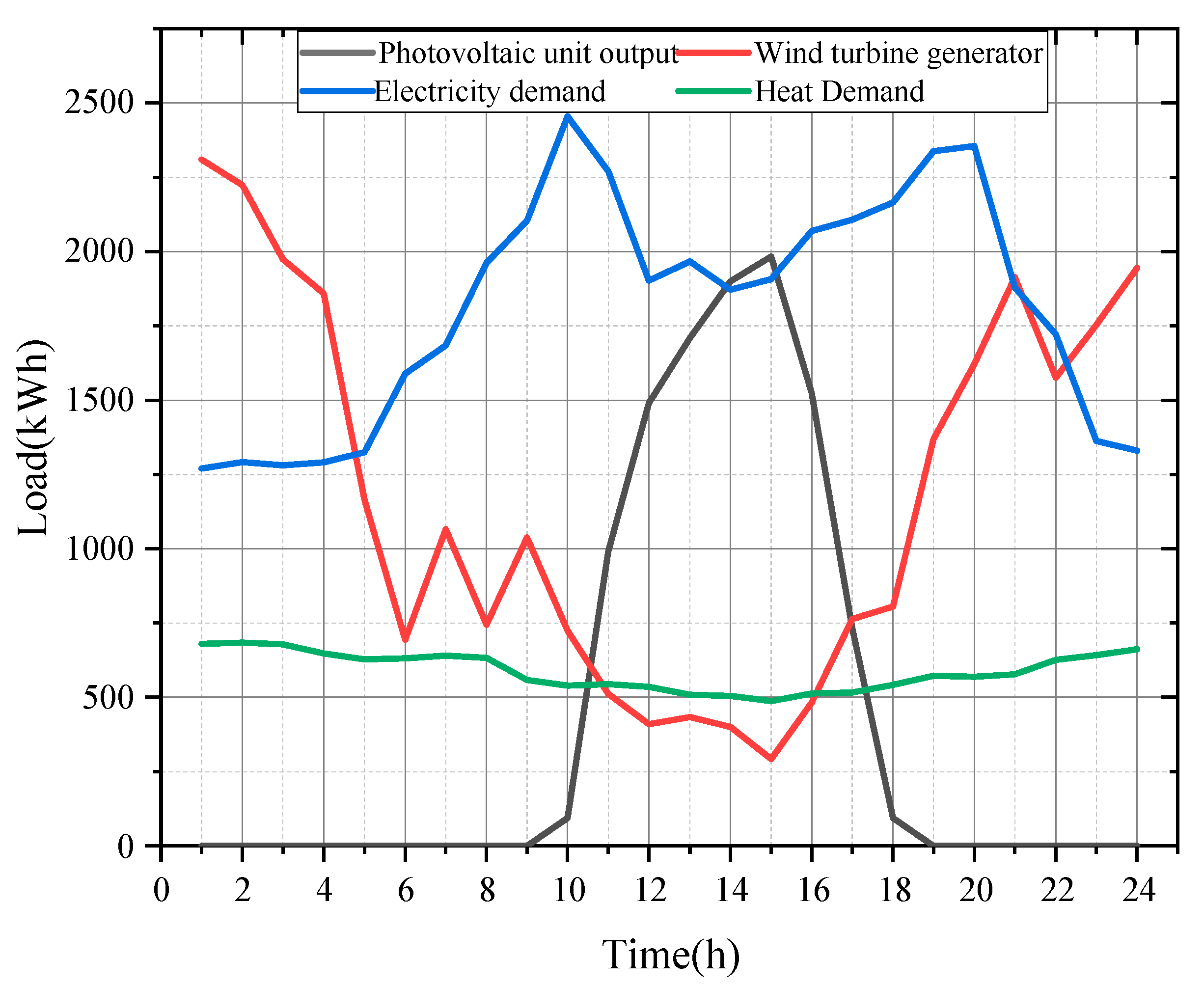
5.1. Simulation Data and Experimental Platform

In this paper, we used the toolbox YALMIP in MATLAB to build an integrated energy microgrid economic optimization model and used the GUROBI solver to solve it. In this paper, we selected a typical regional integrated energy microgrid as the research object. The operation plan was developed based on the constructed IGDT optimization model, an integrated energy microgrid’s optimal economic dispatch model. The scheduling period was 24 h (T = 24), and 1 h was used as a scheduling period. The parameters of the integrated energy microgrid scheduling model are shown in

Table 1. Parameters of integrated energy microgrid scheduling model.

Parameter	Numerical Value	Parameter	Numerical Value
$Q_{ES,0}$ (kWh)	800	$P_{\mathrm{CCS},\min }$ (kW)	0
${\eta }_{ES,c}$	0.95	$P_{\mathrm{CCS},\max }$ (kW)	600
${\eta }_{ES,d}$	0.96	$P_{\mathrm{CHP},\min }$ (kW)	0
$Q_{ES,\min }$ (kWh)	500	$P_{\mathrm{CHP},\max }$ (kW)	2000
$Q_{ES,\max }$ (kWh)	1800	$\alpha$	0.55
$P_{\mathrm{P}2\mathrm{G},\min }$ (kW)	0	$\beta$ (kg/kWh)	1.02
$P_{\mathrm{P}2\mathrm{G},\max }$ (kW)	300	$H_{\mathrm{GB},\min }$ (kW)	0
$P_{k,t}^{\mathrm{buy} }{}_{\max }$ (kW)	500	$H_{\mathrm{GB},\max }$ (kW)	500
$P_{k,t}^{\mathrm{sell} }{}_{\max }$ (kW)	2000	${\eta }_{GB}$	0.9
$c_{\mathrm{v}1}$	0.15	$A$ (kg/kWh)	0.424
$c_{v2}$	0.25	$\epsilon$ (CHY/kg)	0.75
$C_m$	0.82	$\zeta$ (CHY/kWh)	0.01
$a_{{\mathrm{co}}_2}$ (kg/kWh)	0.93	$\mathrm{U}{\mathrm{p}}_{\mathrm{k},\mathrm{t}}^{{\mathrm{CH}}_4}$ (CHY/m3)	2.9
$b_{{\cos }_2}$ (kg/kWh)	0.0015	$c_{\mathrm{P}2\mathrm{G}}$ (CHY/kW)	0.022
$c_{{\mathrm{co}}_2}$	28.79	$d_{\mathrm{P}2\mathrm{G}}$ (CHY/kg)	0.064

. The purchase and sale tariffs of electricity from the integrated energy microgrid to the higher-level primary grid are shown in

Table 2. Microgrid power purchase tariffs.

Time	Electricity Purchase Tariff (CHY/kWh)	Electricity Sales Tariff (CHY/kWh)
Valley hours (23:00–05:00)	0.25	0.2
Weekday periods (06:00–08:00, 12:00–18:00, 21:00–22:00)	0.62	0.2
Valley hours (23:00–05:00)	0.92	0.2

.

Under the typical daily operation and scheduling of an integrated energy microgrid, the forecast of renewable energy generating units’ output and customers’ electricity load for each time are shown in Figure 4.

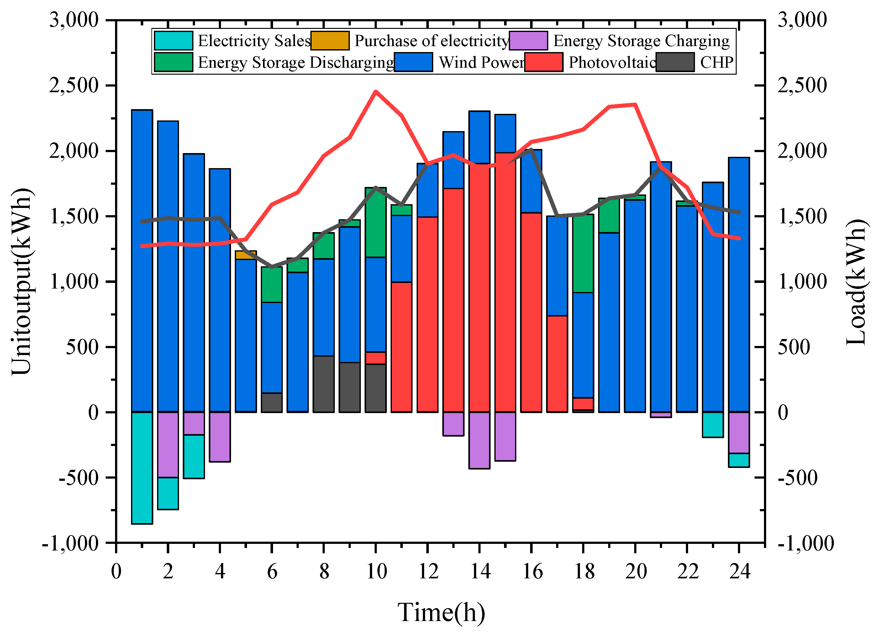
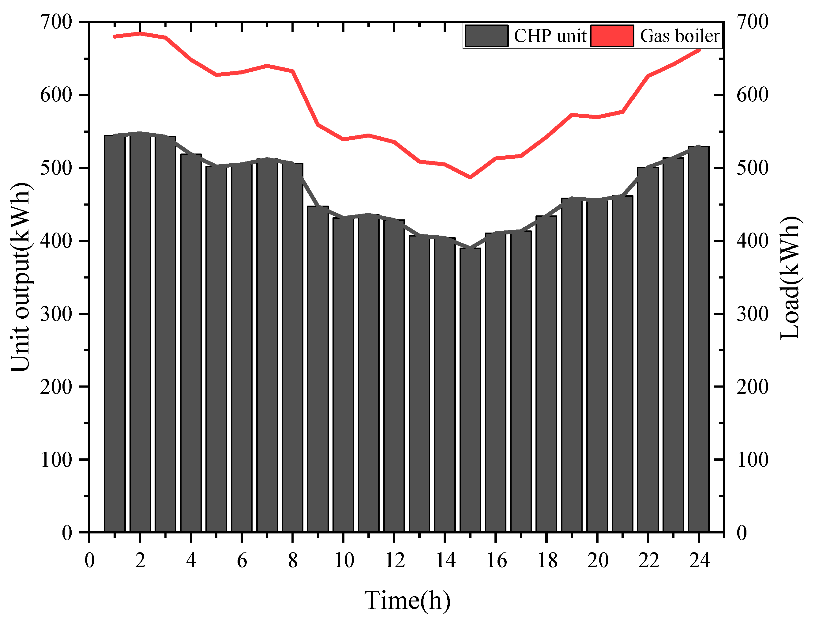
5.2. Scheduling Operation of Integrated Energy Microgrid System under Deterministic Conditions

To verify the effectiveness of low carbon dispatch of integrated energy microgrid with P2G and CCS as proposed, in this chapter, we demonstrate the economics and advantages of P2G and CCS-based integrated energy microgrids regarding carbon emissions through the following four examples.

• Example 1: Integrated energy microgrid without P2G and CCS and carbon trading costs.
• Example 2: Integrated energy microgrid without P2G and CCS but considering carbon trading costs.
• Example 3: Integrated energy microgrid considering P2G and CCS but not carbon trading costs.
• Example 4: Integrated energy microgrid considering P2G and CCS with carbon trading costs.

5.2.1. Comparison of Different Scheduling Results

Figure 5 shows the output of the CHP unit under the different cases. Compared with Example 2, the CHP unit in Example 4 needs to supply energy to the CCS plant and the P2G plant, which reduces the actual output of the CHP unit. Compared with Example 4, the CHP unit in Example 3 only needs to meet the minimum operating requirements of P2G and CCS equipment because it is not limited by carbon emission cost, so it can supply energy to the outside to meet the customer-side demand to the maximum extent.

Figure 6 shows the actual output of WTGs under different cases. During the peak hours of 01:00–04:00 and 20:00–24:00, the actual production of WTGs in Example 2 and Example 3 is significantly smaller than the actual output of WTGs in Example 4, which is because the P2G and CCS devices consume part of the output power of CHP units during operation, which improves the wind power consumption.

Figure 7 shows the carbon emissions for the different scenarios. Example 4 consumes a large amount of CO₂ captured by CCS due to the presence of P2G technology, which reduces the net carbon emissions of the system.

The optimization effects of the different cases are shown in

Table 3. Comparison of the optimization effects of different algorithms.

Example	System Operating Cost/CNY	Wind-Power Consumption	Photovoltaic-Power Consumption	Carbon Emission/kg
Example 1	11,156.38	86.55%	100%	8461.44
Example 2	1076.28	100%	100%	8419.84
Example 3	11,062.12	89.745%	100%	7875.57
Example 4	231.42	100%	100%	3755.63

. By comparing this to Example 2, Example 4 shows that P2G and CCS technologies reduce the carbon emissions of the microgrid while reducing the microgrid system operating costs by CNY 884.86 CNY. Examples 3 and 4 show that the microgrid mainly uses renewable energy as an energy supply, and introducing carbon trading can further reduce the system operation costs.

The relationship between the carbon trading price and the system operating costs under different cases is shown in Figure 8. It can be seen that the system operation cost is not related to the carbon price in Example 1 and Example 3 because the carbon transaction cost is considered, while in Example 2 and Example 4, the system operation cost gradually decreases with the increase in carbon price, which is mainly due to the decrease in carbon transaction cost, and the system operation cost decreases.

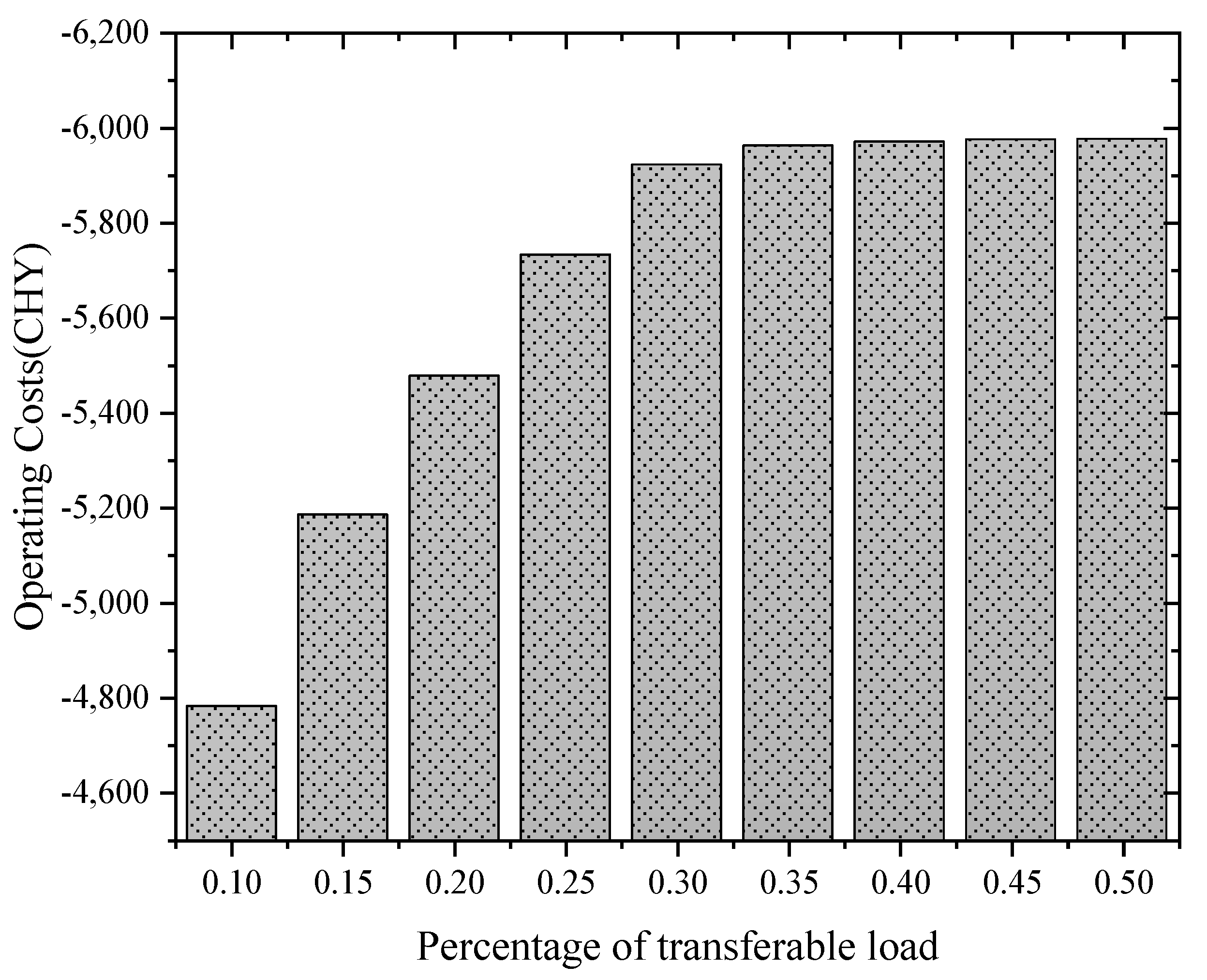
5.2.2. Integrated Energy Microgrid Scheduling Model under C Demand Response

First, the analysis of the microgrid system dispatching operation under deterministic conditions was carried out. The operating parameters of CHP units, gas boilers, and battery storage systems, as well as the predicted values of wind turbine output, P.V. unit output, and electric and thermal load demand before the day, were brought into the microgrid system scheduling operation model, and the total operating cost of the microgrid was CNY −5184.43. At this time, the output of each unit is shown in Figure 9. Figure 8 shows that this microgrid satisfied the customer-side electricity demand while using the demand-response mechanism to reduce the operating cost of the integrated energy microgrid by CNY −5415.85 compared to the operating cost of Example 4. This integrated energy microgrid electric load can respond to time with load shedding or load shifting, further reducing the peak-to-valley difference in electric load by smoothing out electric load fluctuations, realizing the purpose of integrated energy microgrid peak shaving and valley filling, improving the microgrid’s flexible response capability while reducing electric load fluctuation.

Figure 10 shows that 0:00–05:00 and 22:00–24:00 are the peak times of heat consumption by customers. Still, the electric load is in the low time of electricity consumption. The heat output of the CHP unit is low due to the “thermoelectric coupling characteristic” of the CHP unit, so the gas boiler is used to prioritize the demand-side heat consumption. Therefore, gas boilers are operating to meet the demand-side heat demand. During the 07:00–21:00 period, the CHP units can simultaneously work independently to fulfil the demand-side electric and thermal energy demands.

The load share of each type of demand response affects the effect of IDR implementation in an integrated energy microgrid. Based on the deterministic microgrid economic dispatch model, the impact of the share of the curtailable load and transferable load of the microgrid on the operating cost of the microgrid is analyzed.

The relationship between operating cost and the percentage of curtailable demand-response load is shown in Figure 10. Firstly, the transferable bag is kept constant, and the share of the curtailable burden is set from 10 to 50% to analyze the effect of the mobile demand-response load on the operating cost of the microgrid. From Figure 11, it can be seen that the operating cost of the microgrid decreases as the percentage of curtailable demand-response load increases, i.e., the operating cost is negatively related to the curtailable demand-response load, which is due to the reduction of load quantity under the high tariff time, which reduces the energy purchase cost of the microgrid and thus reduces the total operating cost.

The working cost-transferable demand-response load share relationship is shown in Figure 12. From Figure 11, it can be seen that the operating cost of the microgrid decreases as the percentage of transferable demand-response load increases, i.e., the operating cost is negatively related to the curtailable demand-response load, which is mainly achieved by shifting the burden from the high tariff time to the low tariff time, so it is beneficial to improve the operating profit of the microgrid by coordinating the ratio of transferable and curtailable demand-response load.

5.3. Analysis of IGDT Optimization Results

5.3.1. Comparative Analysis of Traditional IGDT Scheduling Results under Seven Uncertain Scenarios

To verify the correctness and accuracy of the IGDT strategy applied to the economic dispatch decision of the microgrid, firstly, different uncertainty scenarios were set for the four uncertainties, including five cases of considering a single uncertainty, only source-load uncertainty, and considering all source-load uncertainties, respectively.

Table 4. Description of the seven uncertainty scenarios.

	Uncertainty of Wind-Power Output	Photovoltaic-Output Uncertainty	Electric-Load Forecast Uncertainty	Uncertainty in Thermal-Load Forecasting
Case 1	◯	×	×	×
Case 2	×	◯	×	×
Case 3	×	×	◯	×
Case 4	×	×	×	◯
Case 5	◯	◯	×	×
Case 6	◯	◯	◯	×
Case 7	◯	◯	◯	◯

illustrates the different combinations of uncertainty parameters in the five scenarios, where “◯” indicates the fate of the factor accounted for in the model, and “×” suggests the uncertainty of the element not accounted for in the model. In particular, this comparative analysis was performed to verify the IGDT strategy’s effectiveness and to evaluate the degree of impact of multiple uncertainties on the system scheduling cost. When considering numerous uncertainties (i.e., Case 5, Case 6, and Case 7), the traditional IGDT model was used for the consistency of the model and to simplify the solution process, using the same uncertainty domain α.

When the robustness level factor varies in the range of 0.01–0.05, i.e., the expected increase in system scheduling cost is within ±5%, the trajectory of the IGDT scheduling model solution results for seven uncertainty scenarios is shown in Figure 13, where the baseline value of the scheduling cost is the value of the scheduling cost obtained from the optimal solution of the deterministic scheduling model. This paper analyzed the results from the perspective of sensitivity to uncertainties.

From the perspective of system dispatching decisions, as the microgrid operating cost increases, i.e., the opportunity level factor decreases and the robust level factor increases, the combined uncertainty in the seven cases of the derived opportunity gradually decreased. In contrast, the combined uncertainty in the substantial opportunity gradually increased. This is mainly due to two very different values of the microgrid management service providers in the face of source-load risk: the opportunity model under the risk-averse strategy considers that uncertainty moves the microgrid in a favorable direction, and the greater the uncertainty α, the more optimistic the microgrid management service provider is about the additional benefits from uncertainty, and the operating cost decreases. Whereas, the robustness under the risk-averse strategy considers that the delay will move the microgrid in an unfavorable direction, and the greater the uncertainty α, the progressively higher the pessimistic value of the additional risk generated by the uncertainty for the microgrid management service provider and the consequent increase in the operating cost.

From the perspective of uncertainty sensitivity, when the robustness level factor is the same, the more significant the robust integrated uncertainty under different uncertainty scenarios, the less sensitive the microgrid is to changes in anticipation, the lower the risk due to delay, and the better the robustness is reflected. In contrast, when the opportunity level factor is the same, the smaller the opportunity-integrated uncertainty under different uncertainty scenarios, the more the microgrid is sensitive, the higher the opportunity gain caused by delay. Figure 12 shows that for the opportunity scheduling model, Case 2 (uncertainty of P.V. generator output) yields the most considerable opportunity-integrated uncertainty, and Case 1 (uncertainty of wind-generator output) yields the slightest opportunity-integrated hesitation under the same level factor. For the robust scheduling model, Case 4 (uncertainty of thermal-load demand) has the highest chance of combined delay, and Case 1 (uncertainty of wind-turbine output) has the lowest opportunity for the same level factor. This is due to the fluctuation of wind power and electric load demand, which are influenced by external conditions. In the risk preference strategy, the limited output of P.V. generating units causes a low operating cost to the microgrids.

In contrast, in the risk-avoidance strategy, the CHP unit supply can satisfy the thermal load, and the CHP unit’s operating cost is low, which has a negligible impact on the operating cost of the microgrid. In addition, the energy storage system in the microgrid can participate in the microgrid economic dispatch as a transferable load, reduce the risk of renewable energy generation to the grid, and provide support for the high percentage of renewable energy to the grid. Limited by its energy storage capacity, it has a limited role in further reducing the dispatching cost.

When the microgrid is operated, the microgrid management service provider will consider the dual source-load uncertainty. Comparing and analyzing the uncertainty curves of Case 5, Case 6, and Case 7 under the scenarios of uncertainty factor combinations, this paper uses the same uncertainty domain α in modelling different uncertainties. It was found that the global optimization results were highly susceptible to the most sensitive uncertainty factors. For example, Case 5 accounts for the delay of wind turbine and P.V. turbine output. The comparison of the curves of Cases 1 and 2 shows that the system is more sensitive to the uncertainty of wind turbine output. Thus, the optimization results of Case 5 are constrained by the fate of wind power, and the resulting curve is very close to Case 1. Similarly, Case 7 considers the uncertainty of wind turbine output, P.V. turbine output, and load demand, and the fate of load demand constrains the optimization results. The result curves are very close to Case 4.

It can be seen that when multiple uncertainties are considered, when the traditional IGDT optimization model is used, the same uncertainty weight is used when the anticipation of different delays is built in, the optimized obtained uncertainty cannot quantify the impact of each uncertainty on the microgrid operation, and the formulated dispatching strategy still has the optimization space. It cannot fully reflect the advantages of the IGDT strategy.

5.3.2. IGDT Scheduling Model Optimization Results Analysis

As described in the previous section, the IGDT microgrid economic dispatch model established in this paper modeled the uncertainty of wind turbine output, P.V. turbine output, and thermal-electric load uncertainty separately and obtained the comprehensive system uncertainty by unifying the tensions of the four in the form of a weighted sum. Assuming that the expected dispatch cost increase in the microgrid system is ±2%, i.e., the cost deviation factor is 0.02, the results of IGDT robust dispatch optimization with different weighting factors are shown in

Table 5. Optimization results of IGDT with different weighting factors.

${\mathsf{\lambda }}_{\mathit{w}}$	${\mathsf{\lambda }}_{\mathit{S}}$	${\mathsf{\lambda }}_{\mathit{E}}$	${\mathsf{\lambda }}_{\mathit{H}}$	${\mathit{\psi }}_{\mathit{O}}$	${\mathit{\psi }}_{\mathit{r}}$
0.25	0.25	0.25	0.25	0.0140	0.0061
0.5	0.2	0.2	0.1	0.0121	0.0051
0.2	0.5	0.2	0.1	0.0148	0.0067
0.2	0.2	0.5	0.1	0.0125	0.0059
0.1	0.2	0.2	0.5	0.0179	0.0071

.

As seen in Table 5, because this microgrid economic dispatch model has different sensitivities to the fluctuations of each uncertainty factor, different weight coefficients will affect the uncertainty solution results of a single uncertainty factor but have little effect on the comprehensive uncertainty of this microgrid economic dispatch model. The weight coefficients do not affect the applicability of the model. The microgrid management service provider can set each weighting coefficient according to the actual situation and historical experience of the system, based on the principle that the higher the sensitivity, the higher the weight coefficient.

The IGDT robust optimization model yields a critical dispatch cost of CNY −5080.74. The uncertainty of wind turbine output is 0.0088, the fate of P.V. turbine output is 0.0035, the anticipation of electric load forecast is 0.0035, the uncertainty of thermal load forecast is 0.0018, and the combined uncertainty of the system is 0.0176. It means that the actual value of the wind turbine output fluctuates by 0.88%, the real value of P.V. turbine output fluctuates by 0.35%, and the genuine demand for electric load deviates within 0.35%. The proper direction of the thermal load varies within 0.18%. The economic dispatch cost of this microgrid does not exceed CNY −5080.74. Currently, the electric power output of each microgrid economic dispatch model unit is shown in Figure 14a. It can be seen that the IGDT robust optimization strategy is more conservative compared with the original dispatching strategy, which is due to the uncertainty of most of the CHP units’ output to cope with the renewable units and demand forecast, which leads to the increase in the operating cost of this microgrid.

The critical dispatch cost derived from the IGDT opportunity optimization model is CNY −5288.12. At this time, the uncertainty of wind turbine output is 0.0035, the anticipation of P.V. turbine output is 0.0014, the uncertainty of electric load forecast is 0.0014, and the fate of thermal load forecast is 0.0007. The comprehensive future of the system is 0.0071. It means that the actual value of wind turbine output fluctuates within 0.35% compared with the predicted value, the real value of P.V. unit output fluctuates by 0.14% compared with the expected value, the genuine demand of electric load deviates within 0.14% compared with the predicted value. The actual direction of the thermal load varies within 0.07% compared with the expected value, and the economic dispatch cost of this microgrid will not exceed CNY −5288.12. At this time, the electric power output of each microgrid economic dispatch model unit is shown in Figure 14b. It can be seen that the IGDT opportunity optimization strategy is more aggressive compared to the original dispatching strategy, which is due to reducing most of the CHP units’ power output in the expectation of increasing the uncertainty in a favorable direction, thus reducing the cost and achieving the desired effect.

It can be seen that the IGDT optimization strategy can quantify uncertainty from two widely different value concepts, risk preference and risk aversion, and provide opportunity optimization models and robust optimization models for microgrid management service providers. In addition, unlike the conventional IGDT optimization model, which can only deal with a single uncertainty, this paper uses a weighted summation approach to simultaneously consider the photovoltaic forecast, wind power forecast, and electric-thermal load forecast uncertainties and to describe the impact of each uncertainty on the microgrid operation cost with a prolonged delay.

6. Conclusions

In this paper, a joint operation model of CHP units with P2G and CCS technologies is proposed. Based on this model, an economic operation model of an integrated energy microgrid taking the demand-response mechanism into account is developed, and the IGDT model is used to simulate the source-load two-side uncertainty to obtain the integrated energy microgrid day-ahead dispatch strategy. Through the analysis of arithmetic cases, the following conclusions were obtained.

(1) The integrated energy microgrid with P2G and CCS technologies can achieve CO₂ capture and utilization, reduce carbon emissions in the microgrid, reduce carbon tax costs and carbon trading costs, and improve the economy of the system; P2G technologies can effectively utilize the excess renewable energy output and enhance the scenery consumption capacity of the integrated energy microgrid.

(2) Demand response can guide users to change their electricity consumption habits according to the scenery output curve, balance the supply and demand during tight periods of electricity consumption, achieve peak and valley reduction in the load curve, and reduce the amount of wind and light abandoned by the system.

(3) The IGDT optimal-dispatching model can effectively solve the uncertainty of renewable energy unit output while achieving the balance of risk control and capital investment for dispatchers by giving a risk-averse power consumption plan. The sensitivity analysis shows that the upper limit of cost reservation and the upper limit of cost release space within the limited uncertainty can be obtained, which is beneficial to the microgrid manager in making a reasonable capital utilization plan.

References

1. Zhao, B.; Sun, L.; Qin, L. Optimization of China’s provincial carbon emission transfer structure under the dual constraints of economic development and emission reduction goals. Environ. Sci. Pollut. Res. Int. 2022, 29, 50335–50351. [Google Scholar] [CrossRef]
2. Amigues, J.-P.; Kama, A.A.L.; Moreaux, M. Equilibrium transitions from non-renewable energy to renewable energy under capacity constraints. J. Econ. Dyn. Control 2015, 55, 89–112. [Google Scholar] [CrossRef] [Green Version]
3. Shang, Y.; Han, D.; Gozgor, G.; Mahalik, M.K.; Sahoo, B.K. The impact of climate policy uncertainty on renewable and non-renewable energy demand in the United States. Renew. Energy 2022, 197, 654–667. [Google Scholar] [CrossRef]
4. Peng, T.; Deng, H. Research on the sustainable development process of low-carbon pilot cities: The case study of Guiyang, a low-carbon pilot city in south-west China. Environ. Dev. Sustain. 2020, 23, 2382–2403. [Google Scholar] [CrossRef]
5. Pang, Q.; Dong, X.; Zhang, L.; Chiu, Y.-h. Drivers and key pathways of the household energy consumption in the Yangtze River economic belt. Energy 2023, 262, 125404. [Google Scholar] [CrossRef]
6. Jiang, Y.; Hu, Y.; Asante, D.; Mintah Ampaw, E.; Asante, B. The Effects of Executives’ low-carbon cognition on corporate low-carbon performance: A study of managerial discretion in China. J. Clean. Prod. 2022, 357, 132015. [Google Scholar] [CrossRef]
7. Endreny, T.; Avignone-Rossa, C.; Nastro, R.A. Generating electricity with urban green infrastructure microbial fuel cells. J. Clean. Prod. 2020, 263, 121337. [Google Scholar] [CrossRef]
8. Mualim, A.; Huda, H.; Altway, A.; Sutikno, J.P.; Handogo, R. Evaluation of multiple time carbon capture and storage network with capital-carbon trade-off. J. Clean. Prod. 2021, 291, 125710. [Google Scholar] [CrossRef]
9. Bi, T.; Zhu, M.; Liu, H. A Powerful Tool for Power System Monitoring: Distributed Dynamic State Estimation Based on a Full-View Synchronized Measurement System. IEEE Power Energy Mag. 2023, 21, 26–35. [Google Scholar] [CrossRef]
10. Neuenkamp, L.; Lewis, R.J.; Koorem, K.; Zobel, K.; Zobel, M.; Botta-Dukát, Z. Changes in dispersal and light capturing traits explain post-abandonment community change in semi-natural grasslands. J. Veg. Sci. 2016, 27, 1222–1232. [Google Scholar] [CrossRef]
11. Liu, H.; Li, J.; Ge, S. Research on hierarchical control and optimization learning method of multi-energy microgrid considering the multi-agent game. IET Smart Grid 2020, 3, 479–489. [Google Scholar] [CrossRef]
12. Zakeri, B.; Syri, S. Electrical energy storage systems: A comparative life cycle cost analysis. Renew. Sustain. Energy Rev. 2015, 42, 569–596. [Google Scholar] [CrossRef]
13. Wang, H.; Zuo, Z.; Wang, Y.; Yang, H.; Hu, C. Estimator-Based Turning Control for Unmanned Ground Vehicles: An Anti-Peak Extended State Observer Approach. IEEE Trans. Veh. Technol. 2022, 71, 12489–12498. [Google Scholar] [CrossRef]
14. Wang, X.; Han, L.; Wang, C.; Yu, H.; Yu, X. A time-scale adaptive dispatching strategy considering the matching of time characteristics and dispatching periods of the integrated energy system. Energy 2023, 267, 126584. [Google Scholar] [CrossRef]
15. Liu, Z.; Xiao, Z.; Wu, Y.; Hou, H.; Xu, T.; Zhang, Q.; Xie, C. Integrated Optimal Dispatching Strategy Considering Power Generation and Consumption Interaction. IEEE Access 2021, 9, 1338–1349. [Google Scholar] [CrossRef]
16. Yang, T.; Zhao, L.; Li, W.; Zomaya, A.Y. Dynamic energy dispatch strategy for an integrated energy system based on improved deep reinforcement learning. Energy 2021, 235, 121377. [Google Scholar] [CrossRef]
17. Zhao, J.; Wen, F.; Xue, S. Stochastic economic dispatch with uncertainty in electric vehicle and wind power output. Power Syst. Autom. 2010, 34, 22–29. [Google Scholar]
18. Dong, C.; Zhao, J.; Wen, F. From Smart Grid to Energy Internet: Basic Concepts and Research Framework. Power Syst. Autom. 2014, 38, 1–11. [Google Scholar]
19. Shahidehpour, M.; Yong, F.; Wiedman, T. Impact of Natural Gas Infrastructure on Electric Power Systems. Proc. IEEE 2005, 93, 1042–1056. [Google Scholar] [CrossRef]
20. Gahleitner, G. Hydrogen from renewable electricity: An international review of power-to-gas pilot plants for stationary applications. Int. J. Hydrog. Energy 2013, 38, 2039–2061. [Google Scholar] [CrossRef]
21. Liu, W.; Wen, S.; Xue, S. Cost characteristics and operating economy analysis of electricity to gas technology. Power Syst. Autom. 2016, 40, 1–11. [Google Scholar] [CrossRef]
22. Kim, B.; Um, T.T.; Suh, C.; Park, F.C. Tangent bundle RRT: A randomized algorithm for constrained motion planning. Robotica 2014, 34, 202–225. [Google Scholar] [CrossRef] [Green Version]
23. Wang, F.; Liu, S.; Chai, Y. Robust counterparts and robust, efficient solutions in vector optimization under uncertainty. Oper. Res. Lett. 2015, 43, 293–298. [Google Scholar] [CrossRef]
24. Peng, C.; Zhang, J.; Chen, L. Coordinated and optimal scheduling of microgrid source-load-storage for calculating and differentiating demand response. Power Autom. Equip. 2020, 40. [Google Scholar] [CrossRef]
25. Liu, D.; Li, Q.; Yuan, X. Optimal scheduling model for microgrid energy considering stochasticity. Power Syst. Prot. Control 2014, 42, 61–65. [Google Scholar]
26. Ding, H.; Gao, F.; Liu, K. Robust optimization-based economic dispatch model for industrial microgrids with wind power. Power Syst. Autom. 2015, 39, 160–167. [Google Scholar]
27. He, Y.; Lyu, Y.; Che, Y. Operational optimization of combined cooling, heat and power system based on information gap decision theory method considering probability distribution. Sustain. Energy Technol. Assess. 2022, 51, 101977. [Google Scholar] [CrossRef]
28. Dai, X.; Wang, Y.; Yang, S.; Zhang, K. IGDT-based economic dispatch considering the uncertainty of wind and demand response. IET Renew. Power Gener. 2018, 13, 856–866. [Google Scholar] [CrossRef]
29. Najafi-Ghalelou, A.; Nojavan, S.; Zare, K. Robust thermal and electrical management of smart home using information gap decision theory. Appl. Therm. Eng. 2018, 132, 221–232. [Google Scholar] [CrossRef]
30. Ma, H.; Liu, Y. Coordinated scheduling decision of wind power climbing events based on IGDT robust model. Chin. J. Electr. Eng. 2016, 36, 4580–4589. [Google Scholar]
31. Tang, L.; Liu, J.; Yang, Y.; Zhou, L. Power purchase and sales strategies of power sales companies under multiple retail contract models based on information gap decision theory. Grid Technol. 2019, 43. [Google Scholar] [CrossRef]
32. Lu, J.; Li, G.; Wu, Z.; Cheng, C. IGDT-based medium-term operational risk measurement method under multi-market of ladder hydropower. Chin. J. Electr. Eng. 2021, 41. [Google Scholar] [CrossRef]
Figure 1. Schematic diagram of integrated energy microgrid system structure.
Energies 16 03314 g001
Figure 2. “Thermal-electrical characteristics” in CCP combined-operation mode.
Energies 16 03314 g002
Figure 3. Flowchart of IGDT scheduling model solution.
Energies 16 03314 g003
Figure 4. Initial load of integrated energy microgrid and projected output of renewable energy generating units.
Energies 16 03314 g004
Figure 5. The output of the CHP unit under different calculations.
Energies 16 03314 g005
Figure 6. The actual output of wind turbines under different calculation cases.
Energies 16 03314 g006
Figure 7. Carbon emissions under different calculations.
Energies 16 03314 g007
Figure 8. Relationship between carbon trading price and system operating cost under different calculations.
Energies 16 03314 g008
Figure 9. The electricity output of each unit in the microgrid economic dispatch model under demand response.
Energies 16 03314 g009
Figure 10. Heat output of each unit in the economic dispatch model of microgrid under demand response.
Energies 16 03314 g010
Figure 11. Operating costs of cuttable demand-response load share relationship.
Energies 16 03314 g011
Figure 12. Operating costs of transferable demand-response load share relationship.
Energies 16 03314 g012
Figure 13. Comparison curves of traditional IGDT scheduling results for seven uncertainty scenarios.
Energies 16 03314 g013
Figure 14. The electricity output of each unit in the microgrid economic dispatch model.
Energies 16 03314 g014