Interrelated Solar and Thermal Plant Autonomous Generation Control Utilizing Metaheuristic Optimization

Abstract

In this study, the load frequency control of a two-area thermal generation system based on renewable energy sources is considered. When solar generation is used in one of the control areas, the system becomes nonlinear and complicated. Zero deviations in the frequencies and the flow of power through the tie lines are achieved by considering load disturbances. A novel grey wolf optimizer, which is a metaheuristic algorithm motivated by grey wolves is utilized for tuning the controller gains. The proportional, integral, and derivative gains values are optimized for the two-area Solar integrated Thermal Plant (STP). As the load connected to the system varies continuously with time, random load variation is also applied to observe the effectiveness of the proposed optimization method. Sensitivity analyses have also been adopted with the deviation in the time constants of different systems. Inertia constant variations of both areas are considered from −25% to +25%, with or without STP. The proposed algorithm shows good dynamic performance as shown from the simulation results in terms of settling time, overshoot values, and undershoot values. The power in the tie line achieves zero deviation quite rapidly in solar-based cases compared to those without STP.

1. Introduction

Automatic Generation Control (AGC) is an essential requirement of power plants for smooth working in the state of load deviations. The control demonstrates that generation in the power system is automatically regulated, which agrees with the changes in loading requirements. The main theme of the AGC study lies in the system frequency regulations. The speed falls with an increment in load demand, and this result in frequency fluctuations [1]. The nature of interrelated solar plants with the already existing thermal plant is to include renewable energy sources in the system. Additionally, the existing grids remain connected with more and more renewable energy sources nowadays. Hence, we have considered the inference of solar PV systems in one of the control areas. This is the primary focus of this proposed work. The necessity of autonomous generation control is one of the essential requirements of the interconnected power system, as continuous load variations are faced by the generation facilities. They are equipped with systems (governors with controllers) to respond like the primary and secondary controls. In these conditions, generation is altered, as per the requirements, through governor controls. Additionally, it is required to achieve zero steady-state deviations in frequencies concerning the control areas. The tie power flow should also have zero steady-state errors.

Nowadays, power systems are interrelated. So, disruption in one of the areas creates a disturbance in another area. Additionally, the control areas are interconnected through tie lines. So, the conditions of AGC are to control both the frequency and the tie-line power at scheduled values. Automatic Generation Control has gained more importance and attention from researchers due to its role in interconnected systems. The main challenge is frequency management since it has a direct connection with speed. If the system frequency changes, the speed of a plant changes, and hence, the output of the power plant is affected. So, the challenge is to nullify the frequency deviations as quickly as possible after a change in the system loading conditions. For fast and efficient controls, the gain of the secondary controller must be properly optimized for achieving zero steady-state errors in frequency and tie-line power flow. Researchers have adopted several optimization algorithms for tuning the gains of secondary controllers. Several frequency regulation optimization and control methods have already been established over the decades.

The authors have identified deregulation situations with load frequency control operational problems and their technical solutions regarding standard algorithms required for the deployment of this critical condition in [2]. Parameterized AGC schemes are explored, including non-linear and linear power model structures, classical and optimal control, along with centralized control. Wind turbines have also been considered for AGC schemes that utilize intelligent control in [3].

The Differential Evolution (DE) approach based on parallel 2-DOF regulator LFC control is discussed with different conditional parameters such as generation rate constraints and a dead band of the governor with delay time in the system modeling [4]. The authors presented numerous classical controllers, such as an integral controller for automated generation controls in a hydro-thermal system. Additionally, the sensitivity method is used for estimating the controller tuning with the optimum parameters and good robustness, considering large deviations in the system loading [5]. To astound the frequency-fluctuations-related problem, a simple PID control procedure, which counterbalances this variability in the system frequency, is utilized in [6]. Controller parameters have been varying along a wide spectrum of load variations using an imperialist competitive algorithm for obtaining the optimum response of frequency in the same by the authors. Dye-sensitized solar cells Z-series connected modules are tested in a greenhouse environment to combine the devices’ high conversion efficiency, robustness, and transparency, as proposed by the authors [7]. An artificial-intelligence-based algorithm termed the Hybrid Neuro-Fuzzy (HNF) method has been presented by the researchers. The proposed regulator has the advantage of being able to handle non-linearities. It is also faster compared to conventional controllers [8]. The setting of control attributes at optimal values of the power systems centered on PSO aimed at the multi-machines system has been suggested in [9]. This author confirmed that the proposed approach is functioning properly in dampening local and inter-area oscillations with large variations in loading situations and system structures.

Researchers are exploring the merging of renewable energy technologies for electrical power generation and controls. Authors have shown the implementation of an ANFIS strategy that employs artificial neural networks (ANN) for autonomous generation control of the three imbalanced hydrothermal systems [10]. An independent hybrid generating system operation with solar thermal power, battery energy storage, diesel generators, solar PV, ultra-capacitors, fuel cells, wind turbine-based generators, flywheel, and aqua electrolyzer is proposed [11]. Metaheuristic optimization algorithms have become quite prominent in different areas of engineering. A combined cycle’s automatic generation control gas turbine generation plant with traditional controller’s parameter tuning is proposed by the authors utilizing the Firefly Algorithm [12]. For two area thermal systems with wide load fluctuations, a Teaching- and Learning-Based Optimization-based algorithm with a 2-Degree of Freedom of PID controller is proposed [13]. For Automatic Generation Control in a deregulated environment, a hybrid-based Teaching–Learning-oriented optimization and pattern-searching methodology is proposed by the authors, and the findings are compared with Genetic Algorithms and Differential Evolution [14].

Renewable energy with better result attainment for the performance of AGC is presented in the work [15]. One of those algorithms is the Grey Wolf Optimizer (GWO), inspired by grey wolves [16]. In this algorithm, the optimizer simulates the key leadership configuration and the hunting procedure of the grey wolves. The leadership pyramid is an imitation using four types of grey wolves, namely alpha, delta, beta, and omega. The authors presented a mathematical prototype to assess the impression of trifling photovoltaic power plants on performance factors considering the economics of a bigger power system [17]. The use of the grey wolf optimization algorithm for the thermal energy systems incorporated in three control areas for the solution AGC problem is proposed by the authors. In the same work, a conventional thermal system with a single-stage turbine (reheat) and adequate generation constraints (rate) is considered. The algorithm estimates the performances of the proportional–integral, integral, and PID controllers with good accuracy [18]. Authors have suggested a quasi-oppositional dragonfly approach for the tuning of PID control attributes by considering the three-area model. The results are shown with the help of time absolute error [19]. A mathematical standard of trivial (rooftop) photovoltaic (PV) generating station has been established by the authors of [20]. The AGC solutions considering the penetration of the different types of electric vehicles in the electric grids along with the power generation are illustrated by the authors of [21,22,23,24]. In the research work [25], the authors suggested an ANN model utilizing the radial basis function for modelling the non-uniform PV system enactments while controlling the frequency variations [26].

In the past, de-rating techniques have been utilized to qualify frequency backing functions in the PVs; now, for the first time, de-rating techniques are employed to manage voltages in the full PV LV distribution systems [27]. For generating the appropriate patterns of charging for the Li-ion batteries, battery modeling and multi-objective constricted dynamic programming techniques are proposed. In the same work, an ensemble biogeography-based optimization approach is employed for the best solutions [28]. Some authors suggested AI-based strategies to extend the life of the battery from both a production and management standpoint. A critical review of cutting-edge AI-based strategies is also provided, considering ANN and ensemble learning [29]. The authors developed an easily understandable ML algorithm for battery manufacturing. It is also demonstrated that the technique can be applied to predict various components of battery capacities, as well as quantify the dynamic impacts and interconnections of the coating factors very efficiently [30]. To adjust the class imbalance and accurately categorize three important quality indicators of electrodes, an efficient RUBoost-centered classifier framework is proposed. Similarly, experimental findings demonstrate that the proposed systems can deal with class inequity difficulties and precisely predict the characteristics of the produced electrode [31]. Being leadless or containing little lead to overcome the problems posed by hazardous lead yield halides, perovskite materials are investigated for use in the photovoltaic system by the authors of [32]. Research has been undertaken to standardize current AI utilizing deep learning operations in this field after the paper first offers a review of AI and big data in combating COVID-19 [33]. The authors have discussed using the stacking CQDs of various sizes; the graded band orientation approach is employed to reduce the charge carrier diffusion in QNR [34]. The exhaustive literature review shows that many researchers have applied different PID controllers for LFC problems. Generally, all have considered simple load variations. In this work, we consider variable and random step load variations in load demands. Additionally, the sensitivity variations of different parameters are examined in a wide range.

Most of the actual-world optimization is inherently nonlinear and multimodal, with a wide range of complicated constraints. Even for a unified purpose, an approach to optimal solutions is always quite impossible. Metaheuristic optimization techniques have gained popularity for solving complex problems that are otherwise challenging to solve using conventional methods. Metaheuristic methods are now being used to find high-quality results for an ever-increasing variety of complex real-world issues, such as combinatorial problems. As these algorithms can handle multi-objective, multi-solution, and non-stationary problems very efficiently.

In the proposed PID controller, the system attributes have been calculated utilizing the metaheuristic algorithm for the estimation of competitive attribute values(parameters). The motivation for this paper is to utilize the metaheuristic algorithm for the tuning of the control parameters of multi-area load frequency control with and without the insertion of renewable energy sources and a wide range of load variations. The cutting-edge Grey Wolf Optimizer (GWO) for obtaining admirable transient and steady-state performances is utilized in this paper. The issue of continuous deficiency of energy possessions is also discussed in this work.

Table 1. Acronyms’ full forms.

Acronym	Stands for
ACE	Area Control Error
AGC	Automatic Generation Control
ANFIS	Adaptive-Network-Based Fuzzy Inference System
ANN	Artificial Neural Network
AVR	Automatic Voltage Regulator
DE	Differential Evolution
DOF	Degree of Freedom
FPC	Flat Plate Collectors
GWO	Grey Wolf Optimizer
I	Integral
ITAE	Integral Time Absolute Error
LFC	Load Frequency Control
PI	Proportional–Integral
PID	Proportional–Integral–Differential
PSO	Particle Swarm Optimization
PTC	Parabolic Trough Collectors
PV	Photovoltaic
SLP	Step Load Perturbance
STP	Solar Thermal Plant

shows the full forms of acronyms used in this paper.

The key contributions of the authors in this article are as follows:

• Integration of the thermal power generations with the renewable generations for the automatic generation controls, considering variable and random step load variation in load demand;
• To achieve the zero-frequency error after the different load variations and maintain the system frequency constant at the specified values using the proposed PID controls;
• Maintaining the tie-line power flows at the specified levels for the different changes in load conditions in different generation facilities using the adopted novel meta-heuristic method;
• Improved dynamic performance regarding the sensitivity analysis as evidenced by simulation results, shown by control parameters such as undershoot value, overshoot value, and settling time.

2. Overview of Autonomous Generation Control

The system’s frequency residues consider variations in active power, whereas changes in reactive power have less impact and are mostly determined by variations in the bus voltage gradient. While the automated voltage regulator (AVR) controls the amount of bus voltage and reactive power, the control loop of the load frequency regulator controls real power and frequency.

In contrast to single-area systems, multi-area frequency management is a more complicated issue to be addressed properly. The frequency inaccuracy of one location is related to the other linked areas in big systems since all systems are connected through tie lines. The following traits are connected to the multi-area system:

• When a single system loses power, a multi-area system allows electricity to flow from one area to another. In this situation, the blackout problems can be mitigated;
• The least amount of frequency variation also gets aggregated.

The fundamental drawback of a multi-area system, despite some of its advantages, is that any disturbance in one area will also create frequent disruptions in the other control area. Every area needs to be in check for things to run normally and effectively.

Two Control Area Systems (Thermal Energy)

Two control regions for thermal (reheat) generating systems have been considered. As shown in Figure 1, both control regions have been subjected to step load changes and governor–turbine systems as their basis. One section has a hard or strong internal connection, while the other has a weak tie-line outward connection. Frequency deviances for areas 1 and 2 are shown as $\Delta w_1$ and $\Delta w_2$, respectively.

All pool members must contribute to the frequency control, without affecting their own net interchange as part of the tie-line-centered bias control scheme. This implies that the frequency variation and the tie power deviation change must attain zero value under steady-state conditions.

ACE is the linear function of inter-area connected lines power fluctuations and frequency instabilities. The relationships given by Equations (1) and (2) illustrates the expressions of ACE for the two control zones:

$$AC{E}_1=\Delta P_{12}+B_1\Delta w_1$$

(1)

$$AC{E}_2=\Delta P_{21}+B_2\Delta w_2$$

(2)

3. Modeling of Solar-Based Thermal Plant

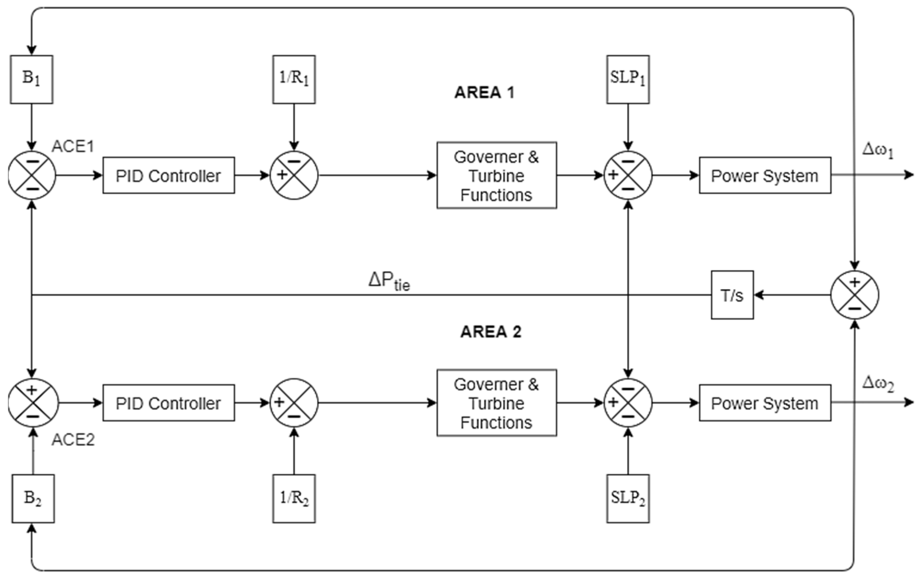
The two most viable sources of renewable power are solar PV and wind generation. The solar collector types utilized in solar-based thermal power plants include Parabolic Trough Collectors (PTC), sterling engines(dish), and Flat Plate Collectors (FPC). To obtain the most solar irradiation, the working fluid is carried by the solar collector. Figure 1 depicts two area systems with thermal (reheat) power plants. These systems have been upgraded to include Solar generation with Thermal Plants generation (STPs) in area 1, while area 2 simply consists of the thermal generation system. For the thermal system, the nominal attribute values were obtained from [1], and for the solar thermal system, the same is taken from [13].

The following abbreviations have been used in the above Figure 1 and Figure 2:

$B_1$ and $B_2$ are the constants for frequency biases in area 1 and area 2;

$R_1$ and $R_2$ are speed directive attributes for governor of area 1 and area 2;

${SLP}_1$ and ${SLP}_2$ are load deviations (step changes) in area 1 and area 2;

${ACE}_1$ and ${ACE}_2$ are ACE in area 1 and area 2;

${∆P}_{tie}$ shows the alteration in tie power flow amid area 1 and area 2;

${∆\omega }_1$ and ${∆\omega }_2$ represent changes in frequency/frequency aberrations in area 1 and area 2.

In Figure 3, arrow ${\mathrm{T}}_{\mathrm{i}}$ indicates the direction of fluid flow. A fluid of temperature ${\mathrm{T}}_{\mathrm{o}}$ is released. I demonstrate the way solar radiation heats pipes and stores energy in working fluid. The symbols used are as follows:

• $T_o$ = collector (outlet fluid) temperature (°C);
• $I$ = solar radiation across collection plane $(\mathrm{W}/{\mathrm{m}}^2)$;
• $T_i$ = collector (inlet fluid) temperature (°C);
• $T_e$ = collector (environment) temperature (°C);
• $v$ = flow rate of collector (or pump) ( ${\mathrm{m}}^3/\mathrm{s}$ );
• ${\eta }_0$ = collector optical efficiency;
• $V_L$ = collector complete heating loss coefficient ${(\mathrm{W}/\mathrm{m}}^2\mathrm{K})$;
• $c$ = heat capacity (specific) of collector fluid $(\mathrm{J}/(\mathrm{k}\mathrm{g}\mathrm{K}\left)\right)$;
• $C$ = $(\rho \ast c\ast V)$, heat capacity of the fluid of collector $(\mathrm{J}/\mathrm{K})$;
• $A$ = surface area of the collector ( ${\mathrm{m}}^2)$;
• $V$ = collector heat transfer volume ${(\mathrm{m}}^3)$;
• $\rho$ = collector (fluid) corpus density ${(\mathrm{k}\mathrm{g}/\mathrm{m}}^3)$.

Collector Model

A simpler solar collector is considered to use a constant fluid flow rate. The value of ${\mathrm{T}}_{\mathrm{o}}\left(\mathrm{t}\right)$ from Equation (3) is substituted in Equation (2).

$$\frac{d{T}_o\left(t\right)}{dt}=\frac{A{\eta }_0}{C}I\left(t\right)-\frac{V_{L}A}{C}\left(T_a\left(t\right)-T_e\left(t\right)\right)+\frac{v\left(t\right)}{V}\left(T_i\left(t\right)-T_o\left(t\right)\right)$$

(3)

Equation (4) represents time requirement of variables:

$$T_a\left(t\right)={(T}_i\left(t\right)+T_o\left(t\right))/2$$

(4)

Then, Equation (2) is arranged in a manner that input parameter is placed on left side, and output parameters are placed in right side, so the new equation is as shown in Equation (5):

$$\frac{d{T}_o\left(t\right)}{dt}+\left(\frac{V_{L}A}{2C}+\frac{v}{V}\right)T_o\left(t\right)=\frac{A{\eta }_0}{C}I\left(t\right)+\left(\frac{v}{V}-\frac{V_{L}A}{2C}\right)T_i\left(t\right)+\frac{V_{L}A}{C}{T}_e\left(t\right).$$

(5)

Applying Laplace transform to Equation (5):

$$L\left[\frac{d{T}_o\left(t\right)}{dt}\right]+\left(\frac{V_{L}A}{2C}+\frac{v}{V}\right)L\left[T_o\left(t\right)\right]=\frac{A{\eta }_0}{C}L\left[I\left(t\right)\right]+\left(\frac{v}{V}-\frac{V_{L}A}{2C}\right)L\left[T_i\left(t\right)\right]+\frac{V_{L}A}{C}L\left[T_e\left(t\right)\right].$$

(6)

Outcome of Laplace transform is shown in Equation (7) as follows:

$$s{T}_0\left(s\right)-T_o\left(0\right)+\left(\frac{V_{L}A}{2C}+\frac{v}{V}\right)T_o\left(s\right)=\frac{A{\eta }_0}{C}I\left(s\right)+\left(\frac{v}{V}-\frac{V_{L}A}{2C}\right)T_i\left(s\right)+\frac{V_{L}A}{C}{T}_e\left(s\right).$$

(7)

Reorganizing Equation (7), we obtain output–input relation, as shown in Equation (8):

$$T_o\left(s\right)=\frac{\tau }{\tau s+1}{T}_o\left(0\right)+\frac{\tau }{\tau s+1}\frac{A{\eta }_0}{C}I\left(s\right)+\frac{\tau }{\tau s+1}\left(\frac{v}{V}-\frac{V_{L}A}{2C}\right)T_i\left(s\right)+\frac{\tau }{\tau s+1}\frac{V_{L}A}{C}{T}_e\left(s\right),$$

(8)

where variable τ represents collector time constant.

Output is assumed by considering only input as $I\left(s\right), T_e\left(s\right)$, and $T_i\left(s\right)$, putting other input zero, and neglecting initial conditions, then we obtain

$$W_1=\frac{T_o\left(s\right)}{I\left(s\right)}=\frac{\tau }{\tau s+1}\frac{A{\eta }_0}{C},$$

(9)

$$W_2=\frac{T_o\left(s\right)}{T_i\left(s\right)}=\frac{\tau }{\tau s+1}\left(\frac{v}{V}-\frac{V_{L}A}{2C}\right),$$

(10)

$$W_3=\frac{T_o\left(s\right)}{T_e\left(s\right)}=\frac{\tau }{\tau s+1}\frac{V_{L}A}{C}.$$

(11)

The effect of initial condition on $T_o\left(s\right)$ is as follows:

$$W_0=\frac{T_o\left(s\right)}{T_0\left(0\right)}=\frac{\tau }{\tau s+1}.$$

(12)

Equation (13) shows individual effect on Equation (10) as follows:

$$T_o\left(s\right)={W_{0}T}_o\left(0\right)+W_{1}I\left(s\right)+W_2{T}_i\left(s\right)+W_3{T}_e\left(s\right).$$

(13)

The transfer rate of heat is assumed to be constant in collector’s model. This transfer function is the output Laplace transform $T_0\left(s\right)$ about the input Laplace transform ($T_i\left(s\right), I\left(s\right), {\mathrm{a}\mathrm{n}\mathrm{d} T}_e\left(s\right))$. Outlet temperature’s initial conditions are selected to make solar field model more realistic.

$$\tau =\frac{1}{\left(\frac{V_{L}A}{2C}+\frac{v}{V}\right)},$$

(14)

where variable τ represents time constant of collector and is also shown by $T_s$.

The difference between input (inlet) and the surrounding temperatures is minimal. Equation (15) shows the function of the solar strength with respect to irradiance (solar):

$$G\left(s\right)=\frac{T_o\left(s\right)}{I\left(s\right)}=\frac{K_s}{1+T_{s}s}.$$

(15)

In the above, variable $K_s$ represents the gain of the collector.

4. Objective Function

The purpose of AGC lies in attaining the zero area control error as fast as possible, as defined in Equations (1) and (2). The time-weighted integration of the absolute value of deviations(ITAE) is utilized for creating the objective function in this present study. It is formulated as the fitness function, as displayed below:

$$f={\displaystyle \underset{0}{\overset{t}{\int }}\left|\Delta w_1-\Delta w_2\right|}.tdt,$$

(16)

where ${∆\omega }_1$ and ${∆\omega }_2$ represent frequency deviations in two areas, i.e., area 1and area 2.

The optimal value is produced via continuous iterative computing. Repetitiveness of the solution is also satisfied to ensure optimal solution.

5. Grey Wolf Procedure for Optimization

The grey wolf method belongs to the class of metaheuristic optimization techniques and is solely employed for calculating the gain constant for optimal outcomes. These metaheuristic schemes have been utilized successfully to tackle several engineering challenges in the real world. The optimization algorithm named GWO approach considers a pack of wolves finding prey and developing better hunting techniques and utilizes the survival of the fittest hypothesis of evolutionary algorithms. The major reason of considering wolf hunting the best is that these wolves dwell in packs. Applications of GWO for resolving the issue of economical load dispatch are discussed in [26].

The social structure and collective hunting strategy of the pack of grey wolves have been given in this paragraph. This algorithm is nature inspired and replicates the clever search method employed by grey wolves for coordination among the group in order to effectively catch prey when hunting. One of the most essential aspects of the grey wolf algorithm is having a rigorous hierarchy at social level, which helps in persevering mutual support with each other at the time of hunting.

Table 2. Hierarchy level of wolfs (in hunting process).

Hierarchy	Rank	Roles
1	α	Main authority, imposes a choice on the pack
2	β	Counselor to Alfa, keep the pack disciplined
3	δ	Guardian of injured wolves
4	Ω	Complies with every pack leader wolf

shows the social structure of wolves with their responsibilities.

5.1. Searching Agents

α, β, δ, and ω represent the search agents. Here, Alpha (α) represents leader, which helps in finding optimal solution during hunting, Beta (β) represents second level optimal result, Delta (δ) is at third level and has less priority compared to α and β, and omega (ω) follows the solution proposed by α, β, and δ and keeps updating its position towards the prey [13]. Equations (17) and (18) are used to obtain the optimal solution.

$$\overrightarrow{D}=\left|\overrightarrow{C}\right.·{\overrightarrow{Y}}_p(k)-\left.\overrightarrow{Y}(k)\right|,$$

(17)

$$\overrightarrow{Y}(k+1)={\overrightarrow{Y}}_p(k)-\overrightarrow{A}·\overrightarrow{D},$$

(18)

where iteration count is k, and $\overrightarrow{Y}(k)$ and ${\overrightarrow{Y}}_p(k)$ are the wolf and prey position vectors, respectively.

$$\overrightarrow{A}=2\overrightarrow{b}·\overrightarrow{s_1}-\overrightarrow{b}$$

(19)

$$\overrightarrow{C}=2·\overrightarrow{s_2}$$

(20)

$\overrightarrow{s_1}$ along with $\overrightarrow{s_2}$ are considered vectors of random nature. The value of $b$ varies between the range of 2 to 0.

$\overrightarrow{C}$ as well as $\overrightarrow{A}$ show location of the prey. For $\overrightarrow{C}$, it may have any value in range of 0 to 2. This indicates the weight of the prey. Considering $\overrightarrow{C}$ is bigger than 1, optimal result is almost achieved. The importance of $\overrightarrow{C}$ is basically for locally optimal point avoidance. During hunting, obstacles may come and be reflected in the random changes in $\overrightarrow{C}$. Value of $\overrightarrow{C}$ maintains the uncertain functioning of GWO, and through this ambiguity, the best outcome is achieved after specific iterations.

$\overrightarrow{A}$ monitors for the prey from first iteration to last iteration. Firstly, one outcome is considered alpha, and then solutions vary from this to find a more suitable result. After best outcome is achieved, convergence is known as to be assisted through $\overrightarrow{A}$.

Divergence occurs when wolves deviate from prey to locate a better prey (|A| > 1). This modernism in $\overrightarrow{A}$ is finished to ensure procedure skillfulness.

Convergence occurs while the result point’s movement is in the best feasible value (1 > |A| > −1) [13].

The first iteration is dedicated to divergence, while the second half is dedicated to position updates towards a point using alpha, beta, and delta as the best points. Figure 4 represents departure from the prey to assimilation to the best ones.

5.2. Positions Apprising

It is assumed that alpha possesses awareness of the ideal while omega wolves’ positions are updating. However, beta with the deltas have knowledge regarding what is the best solution [13]. Using the defined mathematical calculations, omega travels to its next ideal position approaching prey as follows:

$${\overrightarrow{D}}_{\alpha }=\left|{\overrightarrow{C}}_1\right.\cdot {\overrightarrow{Y}}_{\alpha }(k)-\left.\overrightarrow{Y}\right|$$

(21)

$${\overrightarrow{D}}_{\beta }=\left|{\overrightarrow{C}}_2\right.\cdot {\overrightarrow{Y}}_{\beta }(k)-\left.\overrightarrow{Y}\right|$$

(22)

$${\overrightarrow{D}}_{\delta }=\left|{\overrightarrow{C}}_3\right.\cdot {\overrightarrow{Y}}_{\delta }(k)-\left.\overrightarrow{Y}\right|$$

(23)

$${\overrightarrow{Y}}_1={\overrightarrow{Y}}_{\alpha }-{\overrightarrow{A}}_1\cdot \left(\overrightarrow{D_{\alpha }}\right)$$

(24)

$${\overrightarrow{Y}}_2={\overrightarrow{Y}}_{\beta }-{\overrightarrow{A}}_2\cdot \left(\overrightarrow{D_{\beta }}\right)$$

(25)

$$\overrightarrow{Y}(k+1)=\raisebox{1ex}{$(\overrightarrow{Y_1}(k)+\overrightarrow{Y_2}(k)+{\overrightarrow{Y}}_3(\left.k)\right)$}\!\left/ \!\raisebox{-1ex}{$3$}\right..$$

(26)

The three best options have a notion about their prey, the other wolves compute their separation from them that are ${\overrightarrow{D}}_{\delta }$, ${\overrightarrow{D}}_{\alpha }$, and ${\overrightarrow{D}}_{\beta }$ respectively. These distances support establishing the three best feasible placements for omega. The next best locations are updated by averaging such three possibilities.

This position-updating technique is continued until the most optimum point is obtained. This may also be continued until the maximum iteration has been completed and the location has been established after the computations. This process is repeated to ensure that the most recently updated location is the ideal place.

In above Figure 5, circles of dissimilar colors show the prey and the wolves. $a_1,C_1, \mathrm{a}\mathrm{n}\mathrm{d} a_2$ along with $C_2,a_{3,} \mathrm{a}\mathrm{n}\mathrm{d} C_3$ are significant elements for the position of the searching agents. The technique drives omega (hunter) in direction of the estimated location of prey, as displayed in the figure.

5.3. Illustration for Understanding the GWO Procedure

GWO has a goal function for which a random set of populations is generated. In this instance, the aim is to minimize the function. To commence, a random population is created, as indicated in

Table 3. Objective function values for random values of Y1 and Y2.

No. (n)	Y1	Y2	F
I	5.9202	4.0123	6.9806
II	5.8990	5.0009	6.0031
III	7.4190	7.9874	46.0083
IV	3.0018	1.0103	6.0122
V	5.9089	3.3810	3.9909
VI	5.8902	2.9821	2.9982
VII	6.9708	5.8530	23.9081
VIII	5.0072	2.9802	2.0018
IX	4.7900	2.9907	1.9998
X	5.9702	2.9850	3.0021

, and then each collection of population functions is computed. The functions are shuffled in the first iteration to acquire the top three results; this is displayed in

Table 4. Best Solutions.

Results for	Y1	Y2	F
α	5.0013	2.9084	2.0019
β	5.0108	2.9980	3.0201
δ	6.0015	2.9581	3.2039

. Entire leftover solutions are referred to as choices. They are modified in each cycle, as seen below (Equations (27)–(29)):

$$\overrightarrow{b}=2-2\left(\frac{itr}{\max itr}\right).$$

(27)

This gives,

$$\overrightarrow{b}=1.3232$$

(28)

$$\overrightarrow{D}=\left|2rand(0,1)[4.6917,3.2904]\overrightarrow{Y_b}(k)-\overrightarrow{Y}\right|$$

(29)

$$\overrightarrow{Y_1}=[5.0013,2.9084]-(2\overrightarrow{b}·rand (0,1)-\overrightarrow{b}){\overrightarrow{D}}_{\alpha }$$

(30)

$${\overrightarrow{D}}_{\alpha }=\left|2rand(0,1)[5.0108,2.9980]\overrightarrow{Y_b}(k)-\overrightarrow{Y}\right|$$

(31)

$$\overrightarrow{X_2}=[5.0108,2.9980]-(2\overrightarrow{b}·rand (0,1)-\overrightarrow{b}){\overrightarrow{D}}_{\beta }$$

(32)

$${\overrightarrow{D}}_{\alpha }=\left|2rand(0,1)[6.0015,2.9581]\overrightarrow{Y_b}(k)-\overrightarrow{Y}\right|$$

(33)

$$\overrightarrow{Y_3}=[6.0015,2.9581]-(2\overrightarrow{b}·rand (0,1)-\overrightarrow{b}){\overrightarrow{D}}_{\delta }$$

(34)

$$\overrightarrow{Y}(1,:)=\frac{{\overrightarrow{Y}}_1(k)+{\overrightarrow{Y}}_2(k)+{\overrightarrow{Y}}_3(k)}{3}$$

(35)

$$\overrightarrow{Y}=[3.0480,2.6845]$$

(36)

The initial value combination’s position is updated here. Same is performed for the alternative solutions. If the value of omega in the following iteration function is lesser than alpha, these solutions for omega become the subsequent best solution.

$$f_{omega}<f_{alpha}$$

(37)

This technique is repeated until the minimal function value is reached. Figure 6 depicts the flowchart for the suggested grey wolf optimization procedure.

6. Results and Discussion

Results and the corresponding discussions are given in this section.

6.1. Result with STP and without STP

In order to compare the effects of solar energy on the system’s different characteristics in both scenarios with and without STP, solar energy is employed in the power system.

Table 5. Controller gains without and with STP.

Controller Gain	Without STP	With STP
$k_{p,1}$	0.5601	0.7498
$k_{p,2}$	0.7898	0.3311
$k_{i,1}$	0.4084	0.3202
$k_{i,2}$	0.4802	0.3402
$k_{d,1}$	0.4983	0.5387
$k_{d,2}$	0.3456	0.7008

reflects the customized and optimized values for both cases.

As shown in Figure 7, the frequency variation area 1 quickly reaches zero in the case of a solar thermal power plant. Figure 8 displays frequency discrepancy in area 2 and demonstrated improved results in the case of using PV. Figure 9 displays power flow in the tie line without and with STP. The SLP value considered is 0.2. (TH SOURCE—thermal source and STP SOURCE—solar thermal power source)

In the solar thermal instance, fluctuations in the power flow of the tie line attain the desired null value in the least time.

Table 6. Performance attributes dynamics without and with STP (Undershoot—US, Overshoot—OS, and Time to Settle—TS).

Attributes	Performance (Dynamics)	Without STP	Along with STP
∆w1	TS	21.500312	8.649830
	OS	0.0107588	0.001642
	US	0.0007589	0.001342
∆w2	TS	20.989801	9.988071
	OS	0.0106175	0.008796
	US	0.0004987	0.000543
∆Ptie	TS	22.9012341	9.501261
	OS	0.0004598	0.005768
	US	0.00019978	0.0003650

correlates withthe dynamic performances of both systems. It can be concluded that solar power source penetration in area 1, along with the thermal source transient performance, is also quite better in terms of dampening out the frequency and tie-line power deviations to 0.

6.2. Comparison of Results Obtained from GWO with Integral (I) Controllers

The steady-state error is reduced by using integral control. Results show a comparison of integral control with PID control. Grey Wolf Optimization (GWO) is used to optimize the attributes of the PID controller.

Table 7. Performance of GWO tuning compared with PSO [35] and integral tuning (Undershoot—US, Overshoot—OS, and Time to Settle—TS).

Attributes	Dynamics	I Tuning	GWO Tuning	PSO Results
∆w1	TS	24.17865	8.654140	10.3201212
	OS	0.034786	0.002642	0.021235612
	US	0.0076399	0.001242	0.02130346
∆w2	TS	22.64792	10.075095	12.02365781
	OS	0.025696	0.008096	0.00912342
	US	0.0086329	0.0004932	0.00557290
∆Ptie	TS	22.98635	9.48519	14.4785902
	OS	0.0065920	0.006068	0.00608467
	US	0.0089521	0.0004010	0.00149566

shows a comparison of settling time, undershoot values, and overshoot value for various parameter characteristics. It shows that results produced by GWO tuning are much better compared to I tuning.

Jaya algorithm is used to tune PID for STP for comparisons [36].

Table 8. Comparison of I and PI controllers with tuned PID for STP (Undershoot—US, Overshoot—OS, and Time to Settle—TS).

Attributes	Dynamics	I Controller	PI Controller	Tuned PID Control
∆w1	TS	11.92054	14.418729	8.6182208
	OS	0.013824513	0.0123271884	0.003787487
	US	0.035138888	0.021846066	0.021198573
∆w2	TS	14.658047	13.899727	7.6016538
	OS	0.0012796318	0.0016410739	0.00003422029
	US	0.017074277	0.020000111	0.014809222
∆Ptie	TS	24.370994	31.009171	22.898826
	OS	0.014122517	0.0040503251	0.00167344
	US	0.045736824	0.0087653243	0.012513358

shows the comparison between I control, PI control, and tuned PID control.

Below, Figure 10, Figure 11 and Figure 12 give the analogy of dynamic parameters in a chart pattern.

Figure 10 shows the improvement in the settling time of the dynamics in the system using GWO compared to the integral control for two area frequencies and tie-line power deviations. Here, we can see that the settling time is 8.65414 s using GWO compared to 24.17865 s using I control in area 1 frequency changes. Figure 11 shows the improvement in overshoot values using GWO compared to the integral control for two area frequencies and tie-line power deviations. Here, we can see that the overshoot value is merely 0.00264 using GWO compared to 0.034786 using the I control in area 1 frequency changes. Figure 12 shows the improvement in undershoot values in the system using GWO compared to the integral control for two area frequencies and tie-line power deviations. Here, we can see that the undershoot value is 0.00124 using GWO compared to 0.0076399 using I control in area 1 frequency changes.

6.3. Variation in SLP

Figure 13 shows the graph of variable SLP with respect to time. It shows better results compared to those without STP. The incorporation of solar power gives better results with continuously varying SLP also. A variable step (random) load changes are deliberated in area 1 with STP.

The effectiveness of the offered AGC scheme with STP is displayed in Figure 14, Figure 15, Figure 16, Figure 17, Figure 18 and Figure 19. The results show that better results are presented by GWO-based PID controllers (TH SOURCE—thermal source and STP SOURCE—solar thermal power source).

6.4. Sensitivity Investigation

The suggested AGC system is evaluated through sensitivity investigations. Diverse loading scenarios and varied parameters in safe limits are used to analyze the system’s sensitivity. The system without and with STP is used in a wide range of cases for faster dynamic performances. Sensitivity analysis is conducted by varying the parameter fluctuations in the range of −25% to +25%in the parameter shown in

Table 9. Sensitivity investigation results (X = +25% and Y =−25%).

Attribute	% Variation	∆w1	∆w2	∆Ptie
H1	X	7.4991	6.9988	9.5012
	Y	8.0112	9.6014	15.0025
Tg1	X	8.0109	9.0192	8.9873
	Y	9.0017	9.9905	10.9797
Tt1	X	6.7002	8.9782	13.9826
	Y	10.00534	10.9936	11.9837
Ts	X	10.998	11.9935	18.0088
	Y	7.9842	6.0045	5.7681

.

Table 8 shows the attributes regarding variations in collector time constant, turbine time constant, governor time constant, and inertia constants. The collector time constant is less sensitive, and the turbine time constant is the most sensitive. The variations in the frequencies and tie-line power are within safe limits and are almost equal to the nominal values of system attributes. As a result, the given procedure delivers satisfactory, stable, and robust control along with the optimal results of the regulator attributes acquired at standard loading. Additionally, the set values do not need resetting for extensive variations in loading or the parameters.

7. Conclusions

The simulated training using the proposed algorithm in Solar Thermal Plant (STP) is compared with various tuning techniques. Solar PV source is incorporated along with the thermal power system in area 1. The proposed system will be implemented in electrical grids, where the penetrations of renewable sources increase along with traditional thermal generations. It results in less pollution and higher efficiencies. The findings using GWO along with PID reflected faster transient performance compared with simple control (I control).The simulation outcomes demonstrate that using the GWO-optimized PID tuning for solar PV-based two-area thermal generation systems, the fluctuation dynamics die out faster. The settling time is 8.65414 s using GWO compared to 24.17865 s using I control in area 1 frequency changes. Additionally, random step load and the percentage adjustments in the inertia are considered for testing the resilience of system operation. The system parameters such as T_g1, H, T_t1, and T_s were adjusted with a 25% augmentation and reduction for the sensitivity study of autonomous generation control using GWO. Because a 25% fluctuation is probable, the algorithm’s sensitivity is tested for this change. The limitation of this present work is regarding the convergence speed, which may be further improved by using dynamic weights.

In this present work, incorporation of the solar PV with the thermal plant by the submission of GWO-optimized controllers for the two area systems is deliberated. The work may be extended in future with the insertion of EVs with AGC of multi-area systems for optimal control parameters tuning. Additionally, researchers may adopt hybrid optimization algorithms for optimal parameter setting with the inclusion of wind sources and storage.

References

1. Elgerd, O.I.; Fosha, C. The Megawatt-Frequency Control Problem: A New Approach via Optimal Control Theory. IEEE Trans. Power Appar. Syst. 1970, PAS-89, 563–577. [Google Scholar]
2. Christie, R.D.; Bose, A. Load Frequency Control Issues in Power System Operation after Deregulation. IEEE Trans. Power Syst. 1996, 11, 1191–1200. [Google Scholar] [CrossRef]
3. Kumar, P.; Kothari, D.P. Recent philosophies of automatic generation control strategies in power systems. IEEE Trans. Power Syst. 2005, 20, 346–357. [Google Scholar]
4. Kumar, S.R.; Panda, S.; Rout, U.K. DE optimized parallel 2-DOF PID controller for load frequency control of power system with governor dead-band nonlinearity. Electr. Power Energy Syst. 2013, 49, 19–33. [Google Scholar]
5. Chandra, S.L.; Nanda, J.; Mishra, S. Performance comparison of Several classical controllers in AGC for multi-area interconnected thermal system. Int. J. Electr. Power Energy Syst. 2011, 33, 394–401. [Google Scholar]
6. Hamed, S.; Behrooz, V.; Majid, E. A robust PID controller based on imperialist competitive algorithm for load-frequency control of power systems. ISA Trans. 2013, 52, 88–95. [Google Scholar]
7. Barichello, J.; Vesce, L.; Mariani, P.; Leonardi, E.; Braglia, R.; Di Carlo, A.; Canini, A.; Reale, A. Stable semi-transparent dye-sensitized solar modules and panels for greenhouse application. Energies 2021, 14, 6393. [Google Scholar] [CrossRef]
8. Panda, G.; Panda, S.; Ardil, C. Hybrid neuro fuzzy approach for automatic generation control of two-area interconnected power system. Int. J. Comput. Intell. 2009, 5, 80–84. [Google Scholar]
9. Abido, M.A. Optimal design of power-system stabilizers using particle swarm optimization. IEEE Trans. Energy Convers. 2002, 17, 406–413. [Google Scholar] [CrossRef]
10. Khuntia, S.R.; Panda, S. Simulation study for automatic generation control of a multi-area power system by ANFIS approach. Appl. Soft Comput. 2012, 12, 333–341. [Google Scholar] [CrossRef]
11. Das, D.C.; Roy, A.K.; Sinha, N. GA based frequency controller for solar thermal-diesel-wind hybrid energy generation/energy storage system. Int. J. Electr. Power Energy Syst. 2012, 43, 262–279. [Google Scholar] [CrossRef]
12. Saikia, L.C.; Sahu, S.K. Automatic generation control of a combined cycle Gas Turbine plant with classical controllers using Firefly Algorithm. Electr. Power Energy Syst. 2013, 53, 27–33. [Google Scholar] [CrossRef]
13. Sahu, R.K.; Panda, S.; Rout, U.K.; Sahoo, D.K. Teaching learning based optimization algorithm for automatic generation control of power system using 2-DOF PID controller. Int. J. Elect. Power Energy Syst. 2016, 77, 287–301. [Google Scholar] [CrossRef]
14. Khamari, D.; Sahu, R.K.; Gorripotu, T.S.; Panda, S. Automatic generation control of power system in deregulated environment using hybrid TLBO and pattern search technique. Ain. Shams. Eng. J. 2020, 11, 553–573. [Google Scholar] [CrossRef]
15. Buzás, J.; Kicsiny, R. Transfer functions of solar collectors for dynamical analysis and control design. Renew. Energy 2014, 68, 146–155. [Google Scholar] [CrossRef]
16. Mirjalili, S.; Mirjalili, S.M.; Lewis, A. Grey wolf optimizer. Adv. Eng. Softw. 2014, 69, 46–61. [Google Scholar] [CrossRef] [Green Version]
17. Asano, H.; Yajima, K.; Kaya, Y. Influence of photovoltaic power generation on required capacity for load frequency control. IEEE Trans. Energy Convers. 1996, 11, 188–193. [Google Scholar] [CrossRef]
18. Sharma, Y.; Saikia, L.C. Automatic generation control of a multi-area ST-Thermal power system using Grey Wolf Optimizer algorithm based classical controllers. Int. J. Electr. Power Energy Syst. 2015, 73, 853–862. [Google Scholar] [CrossRef]
19. Vedik, B.; Kumar, R.; Deshmukh, R.; Verma, S.; Shiva, C.K. Renewable energy-based load frequency stabilization of interconnected power systems using quasi-oppositional dragonfly algorithm. J. Control. Autom. Electr. Syst. 2021, 32, 227–243. [Google Scholar] [CrossRef]
20. Reddy, V.S.; Kaushik, S.C.; Ranjan, K.R.; Tyagi, S.K. State-of-the-art of solar thermal power plants-A review. Renew. Sustain. Energy Rev. 2013, 27, 258–273. [Google Scholar] [CrossRef]
21. Babaei, F.; Safari, A. SCA based fractional-order PID controller considering delayed EV aggregators. J. Oper. Autom. Power Eng. 2020, 8, 75–85. [Google Scholar]
22. Liu, H.; Yang, Y.; Qi, J.; Li, J.; Wei, H.; Li, P. Frequency droop control with scheduled charging of electric vehicles. IET Gener. Transm. Distrib. 2017, 11, 649–656. [Google Scholar] [CrossRef]
23. Latif, A.; Pramanik, A.; Das, D.C.; Hussain, I.; Ranjan, S. Plug in hybrid vehicle-wind-diesel autonomous hybrid power system: Frequency control using FA and CSA optimized controller. Int. J. Syst. Assur. Eng. Manag. 2018, 9, 1147–1158. [Google Scholar] [CrossRef]
24. Pham, T.N.; Trinh, H. Load frequency control of power system with an electric vehicle and diverse transmission links using distributed functional observers. IEEE Trans. Smart Grid 2016, 7, 238–252. [Google Scholar] [CrossRef]
25. Bakeer, A.; Magdy, G.; Chub, A.; Bevrani, H. A sophisticated modeling approach for photovoltaic systems in load frequency control. Int. J. Electr. Power Energy Syst. 2022, 134, 107330. [Google Scholar] [CrossRef]
26. Pradhan, M.; Roy, P.K.; Pal, T. Grey wolf optimization applied to economic load dispatch problems. Int. J. Electr. Power Energy Syst. 2016, 83, 325–334. [Google Scholar] [CrossRef]
27. Verma, P.; Katal, N.; Sharma, B.; Chowdhury, S.; Mehbodniya, A.; Webber, J.L.; Bostani, A. Voltage Rise Mitigation in PV Rich LV Distribution Networks Using DC/DC Converter Level Active Power Curtailment Method. Energies 2022, 15, 5901. [Google Scholar] [CrossRef]
28. Liu, K.; Zou, C.; Li, K.; Wik, T. Charging pattern optimization for lithium-ion batteries with an electrothermal-aging model. IEEE Trans. Ind. Inform. 2018, 14, 5463–5474. [Google Scholar] [CrossRef]
29. Liu, K.; Wei, Z.; Zhang, C.; Shang, Y.; Teodorescu, R.; Han, Q.L. Towards long lifetime battery: AI-based manufacturing and management. IEEE/CAA J. Autom. 2022, 9, 1139–1165. [Google Scholar] [CrossRef]
30. Liu, K.; Niri, M.F.; Apachitei, G.; Lain, M.; Greenwood, D.; Marco, J. Interpretable machine learning for battery capacities prediction and coating parameters analysis. Control Eng. Pract. 2022, 124, 105202. [Google Scholar] [CrossRef]
31. Liu, K.; Hu, X.; Meng, J.; Guerrero, J.M.; Teodorescu, R. RUBoost-based ensemble machine learning for electrode quality classification in Li-ion battery manufacturing. IEEE/ASME Trans. Mechatron. 2021, 27, 2474–2483. [Google Scholar] [CrossRef]
32. Pandey, R.; Sharma, S.; Madan, J.; Sharma, R. Numerical simulations of 22% efficient all-perovskite tandem solar cell utilizing lead-free and low lead content halide perovskites. J. Micromech. Microeng. 2021, 32, 014004. [Google Scholar] [CrossRef]
33. Manoj, A.; Shweta, A. A systematic review on artificial intelligence/deep learning applications and challenges to battle against COVID-19 pandemic. Disaster Adv. 2021, 14, 90–99. [Google Scholar]
34. Pandey, R.; Khanna, A.; Singh, K.; Patel, S.K.; Singh, H.; Madan, J. Device simulations: Toward the design of> 13% efficient PbS colloidal quantum dot solar cell. Sol. Energy 2020, 207, 893–902. [Google Scholar] [CrossRef]
35. Kennedy, J.; Eberhart, R. Particle swarm optimization. In Proceedings of ICNN’95-International Conference on Neural Networks 1995, Perth, WA, Australia, 27 November–1 December 1995; IEEE: New York, NY, USA, 2002; Volume 4, pp. 1942–1948. [Google Scholar]
36. Bhongade, S.; Paramar, V.P. Automatic generation control of two-area ST-Thermal power system using jaya algorithm. Int. J. Smart Grid 2018, 2, 99–110. [Google Scholar]
Figure 1. Block diagram of two-area thermal system.
Energies 16 03355 g001
Figure 2. Block representation for two area thermal systems with Solar PV source in area 1.
Energies 16 03355 g002
Figure 3. Model of collector.
Energies 16 03355 g003
Figure 4. Convergence action and divergence action [13].
Energies 16 03355 g004
Figure 5. Updating process of the positions of the wolves.
Energies 16 03355 g005
Figure 6. Flow diagram of the proposed algorithm.
Energies 16 03355 g006
Figure 7. Changes in frequency in area 1 without and with STP (SLP two percent).
Energies 16 03355 g007
Figure 8. Changes in frequency in area 2 without and with STP (SLP two percent).
Energies 16 03355 g008
Figure 9. Power flow in tie line without and with STP (SLP two percent).
Energies 16 03355 g009
Figure 10. Settling time variations in I and PID controllers.
Energies 16 03355 g010
Figure 11. Overshoot variations in I and PID controllers.
Energies 16 03355 g011
Figure 12. Undershoot variations in I and PID controllers.
Energies 16 03355 g012
Figure 13. SLPs variations with time scale.
Energies 16 03355 g013
Figure 14. Frequency variations of area 1 without and with STP and variable SLP.
Energies 16 03355 g014
Figure 15. Frequency variations of area 2 without and with STP and variable SLP.
Energies 16 03355 g015
Figure 16. Power flow fluctuations in tie line without and with STP and variable SLP.
Energies 16 03355 g016
Figure 17. Variations of settling time with step load perturbation.
Energies 16 03355 g017
Figure 18. Undershoot variations with step load perturbation.
Energies 16 03355 g018
Figure 19. Overshoot variations through step load agitation.
Energies 16 03355 g019