
Multi-Objective Structural Optimization of a Composite Wind Turbine Blade Considering Natural Frequencies of Vibration and Global Stability
 and
and
Abstract
:1. Introduction
2. The Multi-Objective Structural Optimization Problem
2.1. MOSOPs Formulations
- The MOSOP1 is given by:
- The MOSOP2 is given by:
- The MOSOP3 is given by:
- The MOSOP4 is given by:
2.2. The Optimization Framework
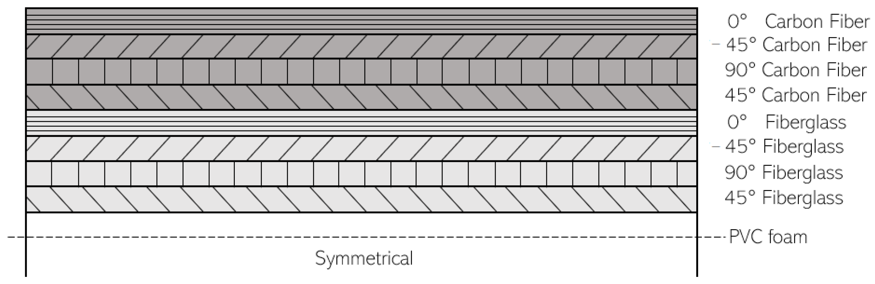
2.3. Design Variables
- (R1) Disorientation rule: The maximum angle offset between two consecutive plies is 45.
- (R2) Laminate balancing rule: The laminate must be balanced with respect to the 0 direction, which implies the same number of 45 and −45 plies.
- (R3) Symmetrical laminate rule: to avoid the in-plane traction and bending coupling.
2.4. Design Constraints
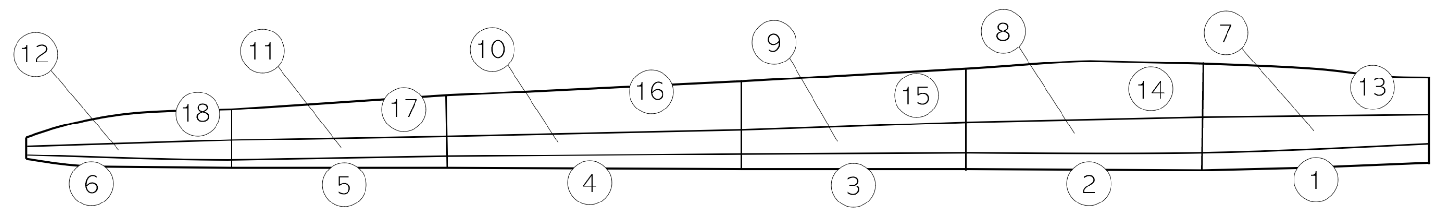
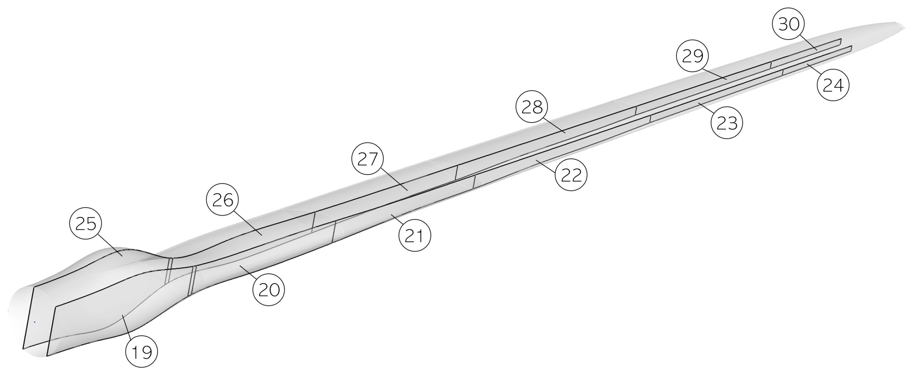
3. Geometric Model of the Blade
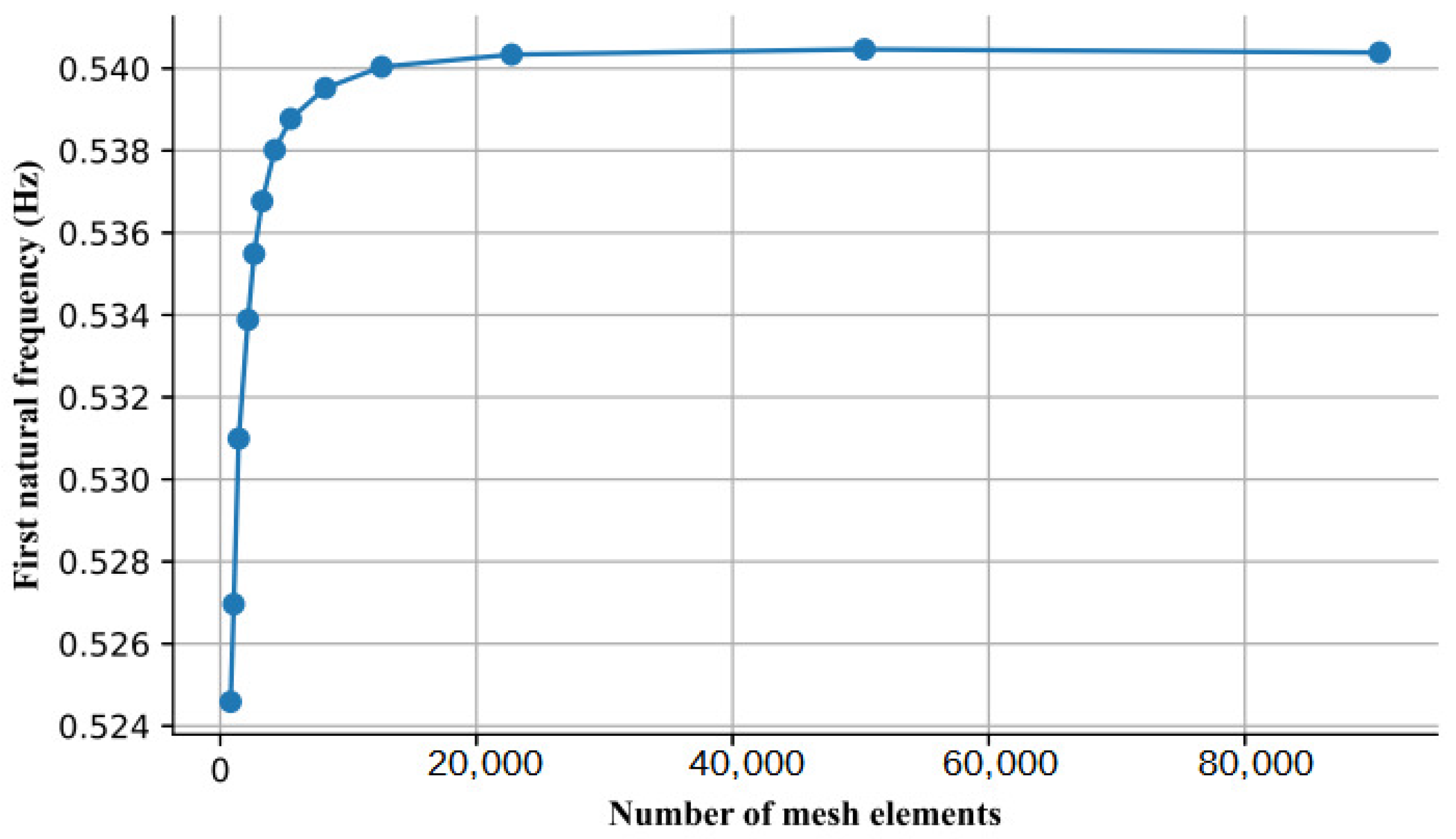
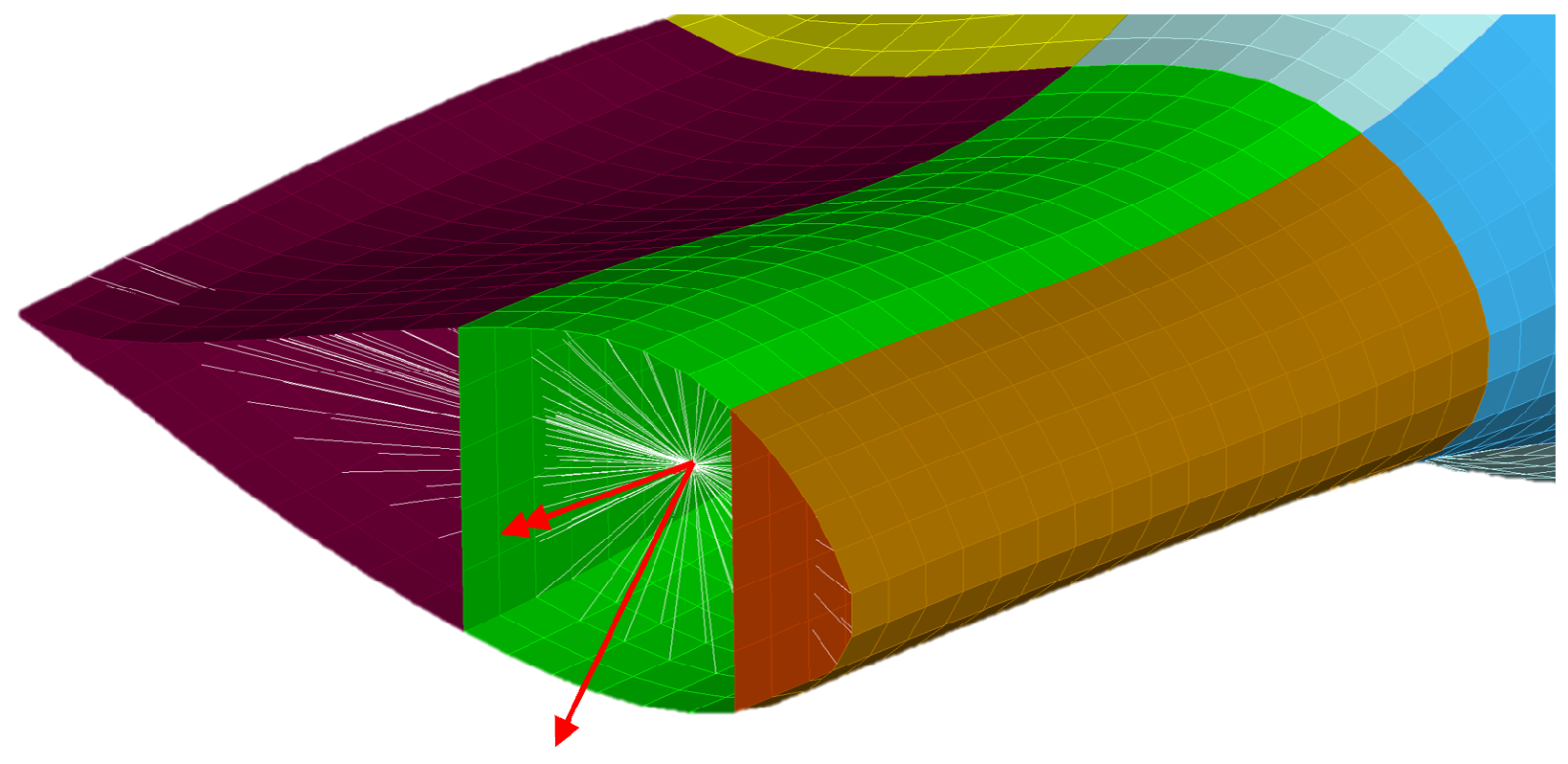
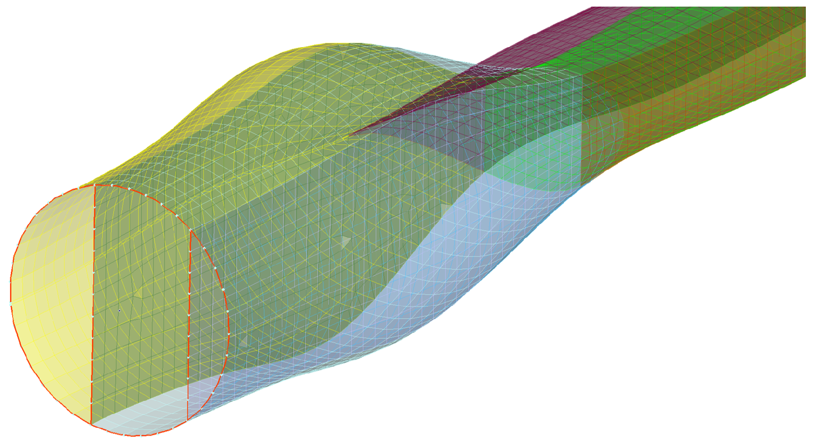
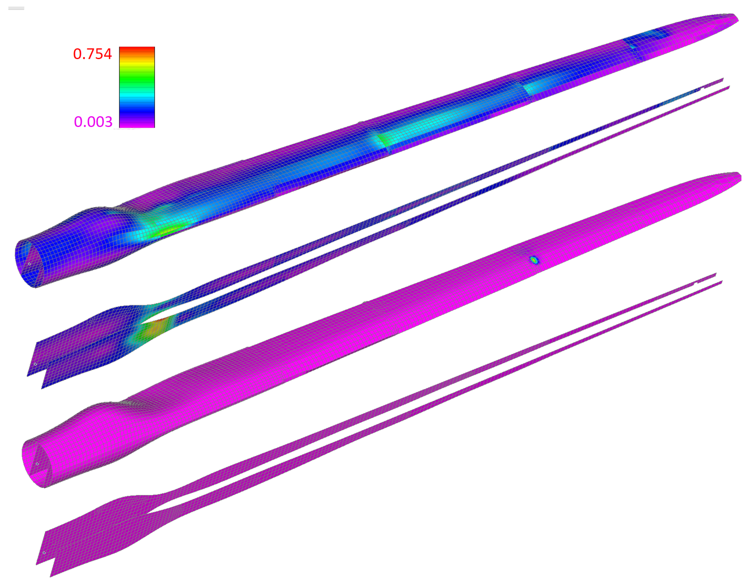
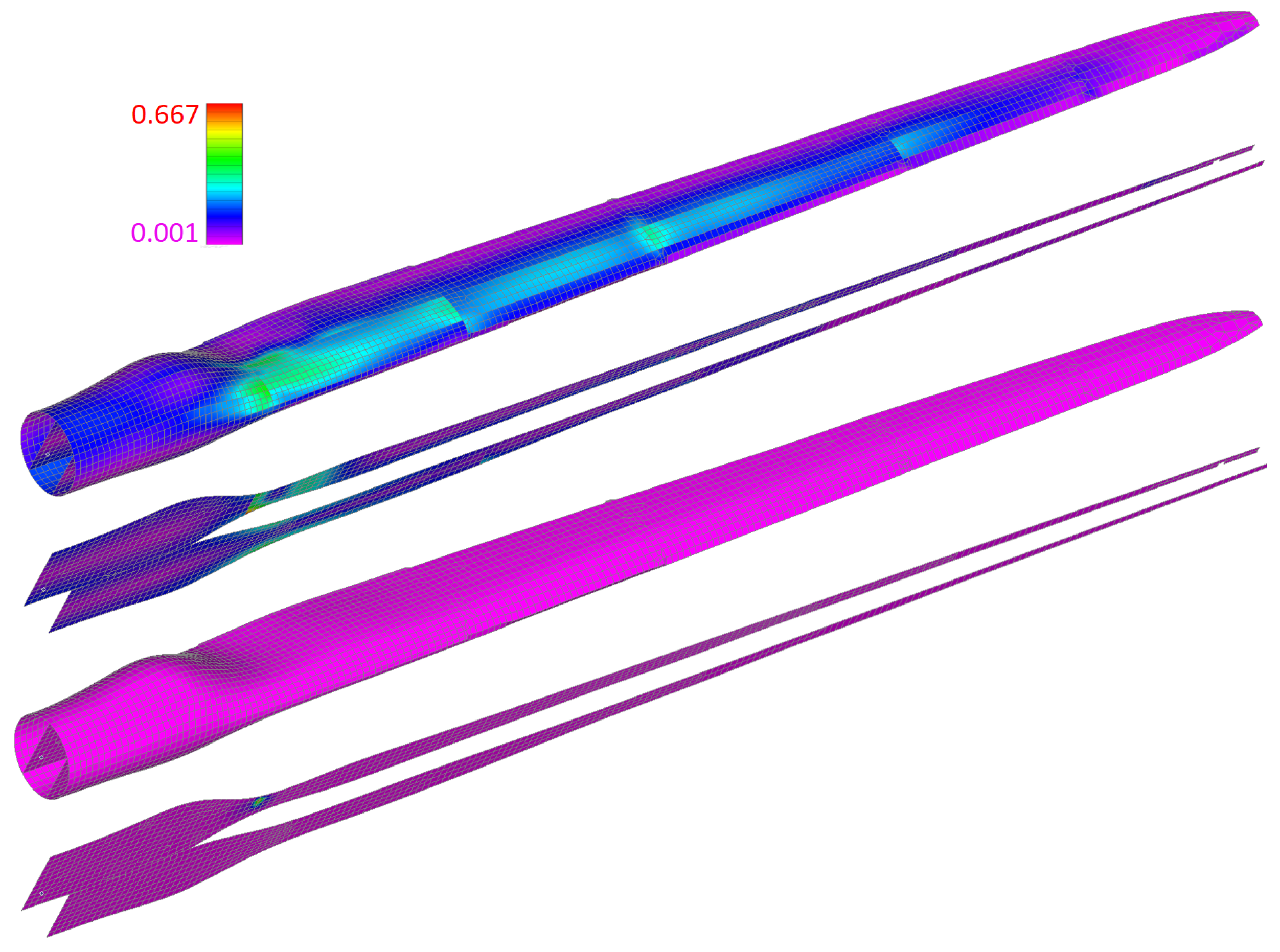
3.1. Finite Element Model
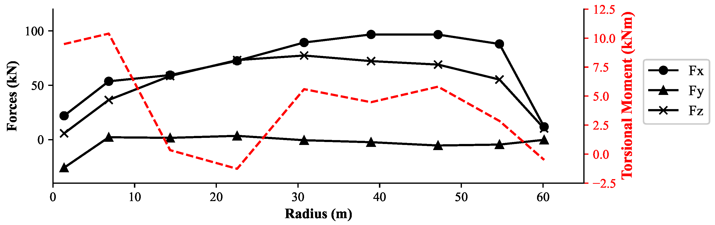
3.2. Load Conditions
4. NSGA-II and Performance Indicators
4.1. Performance Indicators
4.1.1. Hypervolume
4.1.2. Spacing
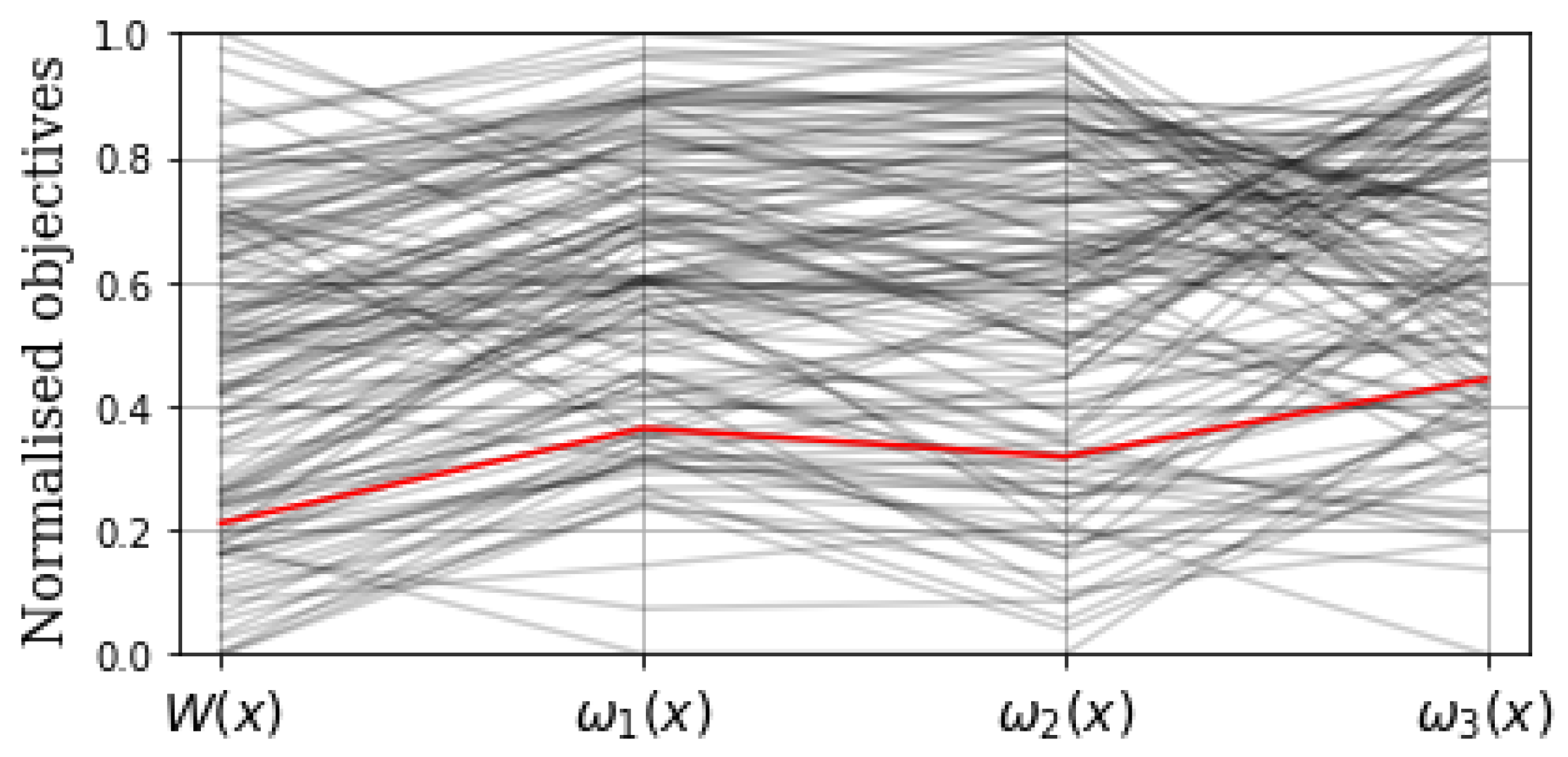
4.2. Multi-Criteria Decision Making (MCDM)
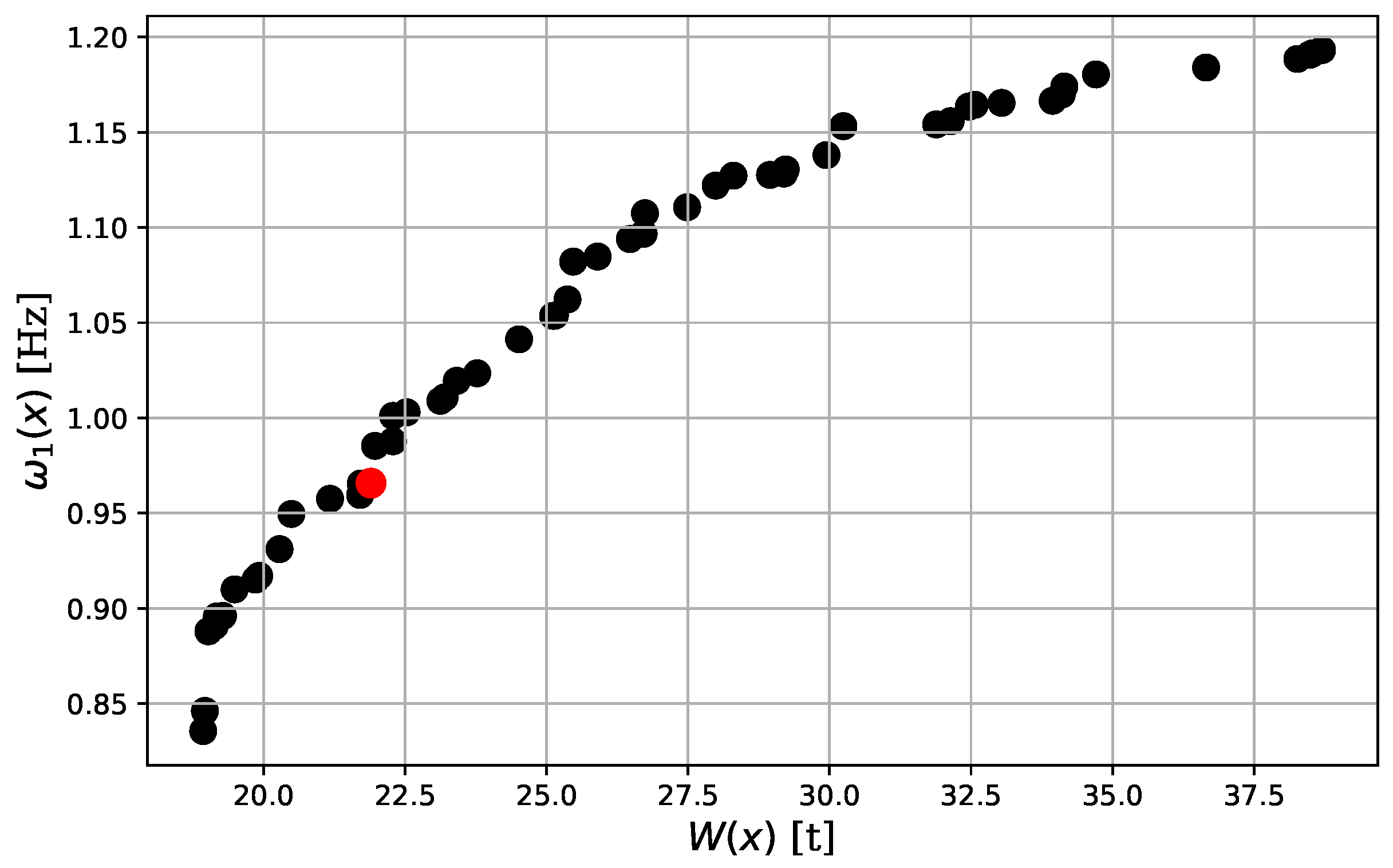
5. Experiments, Results and Discussion

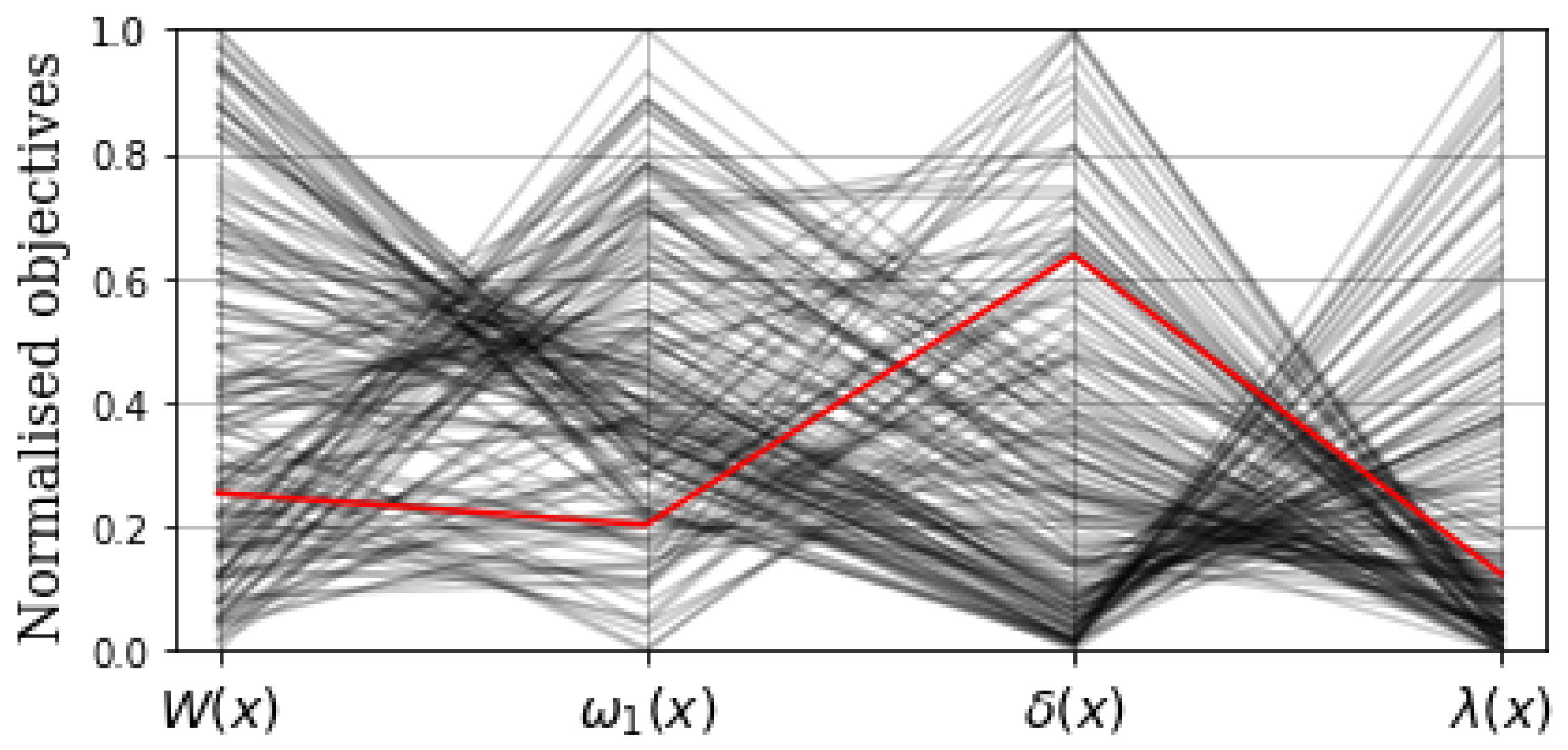
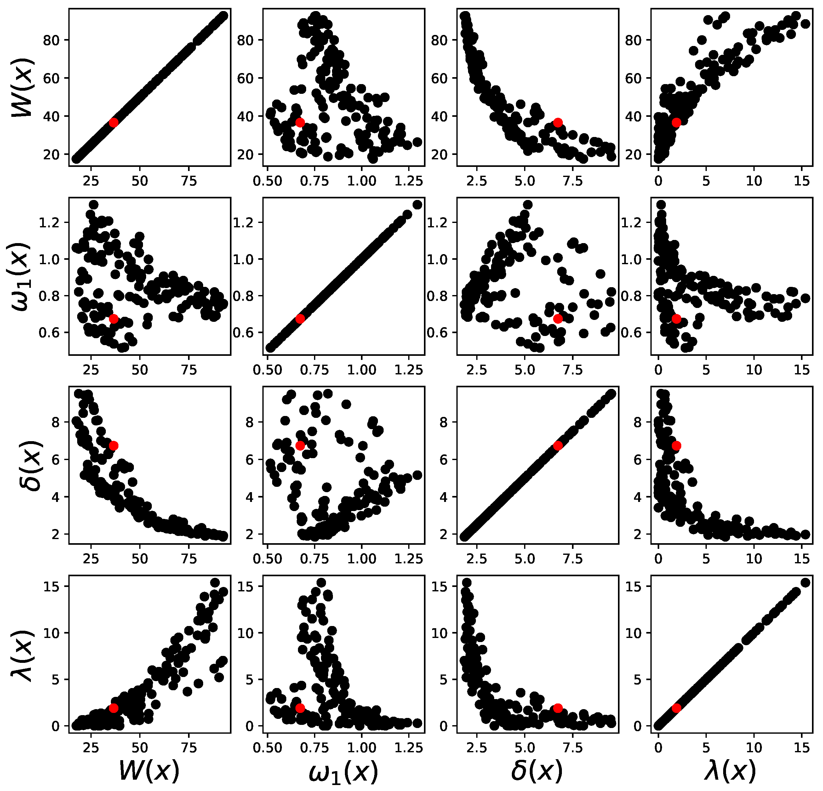
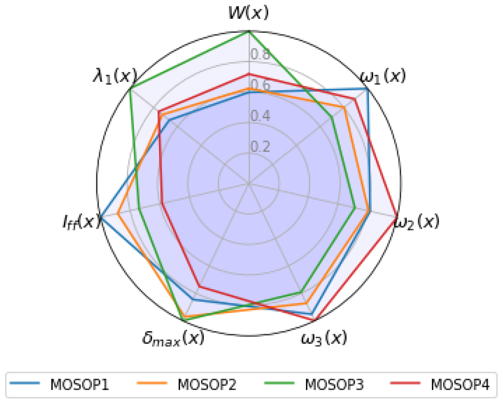
| MOSOP | () | HV | SP | for MCDM () |
|---|---|---|---|---|
| 1 | (100; −0.1) | 86.64 | 0.253 | (0.7; 0.3) |
| 2 | (100; −0.1; 20) | 948.26 | 0.473 | (0.6; 0.2; 0.2) |
| 3 | (100; −0.1; 20; 0) | 5838.47 | 0.854 | (0.4; 0.2; 0.2; 0.2) |
| 4 | (100; −0.1; −0.1; −0.1) | 619.69 | 0.2 | (0.4; 0.2; 0.2; 0.2) |
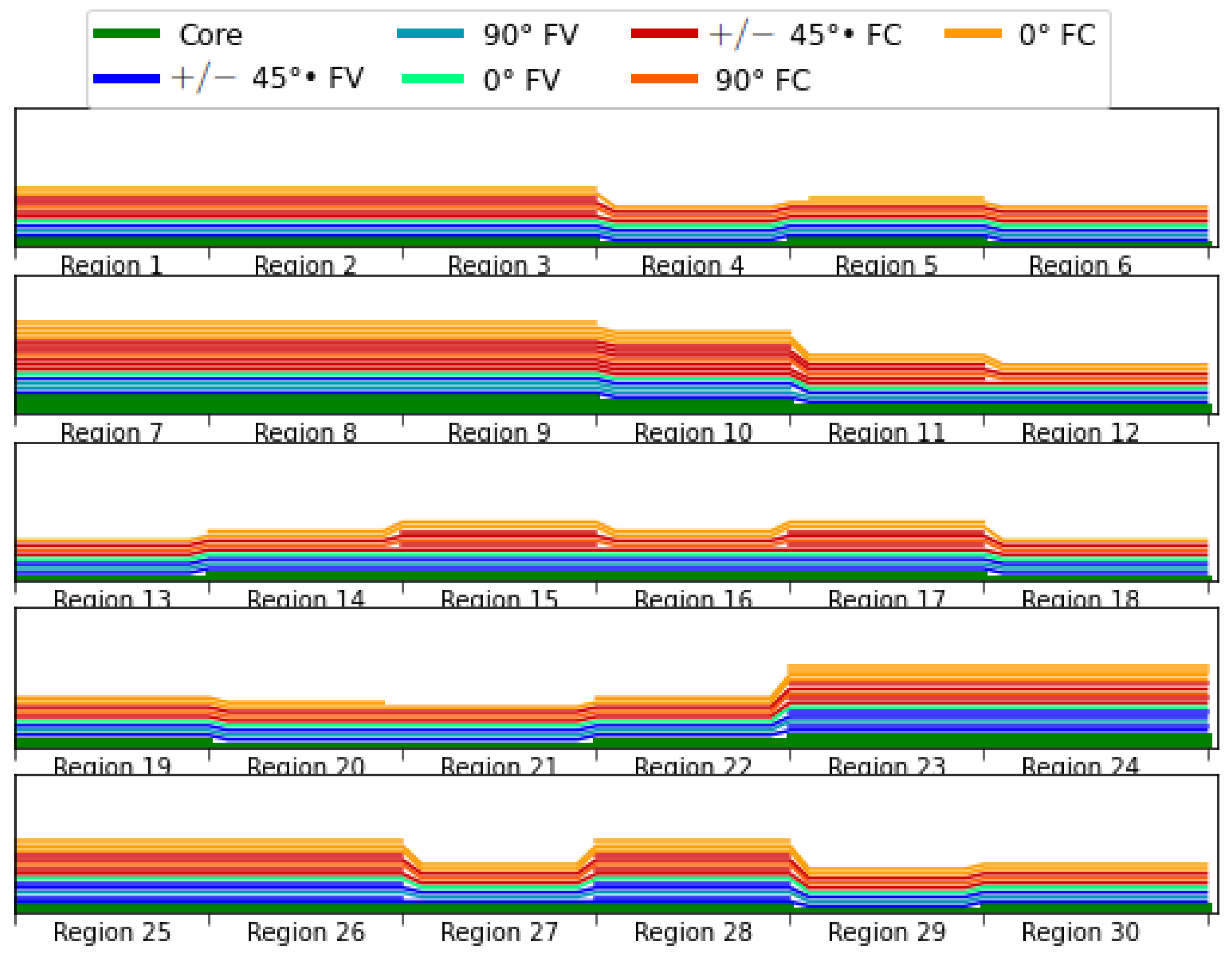
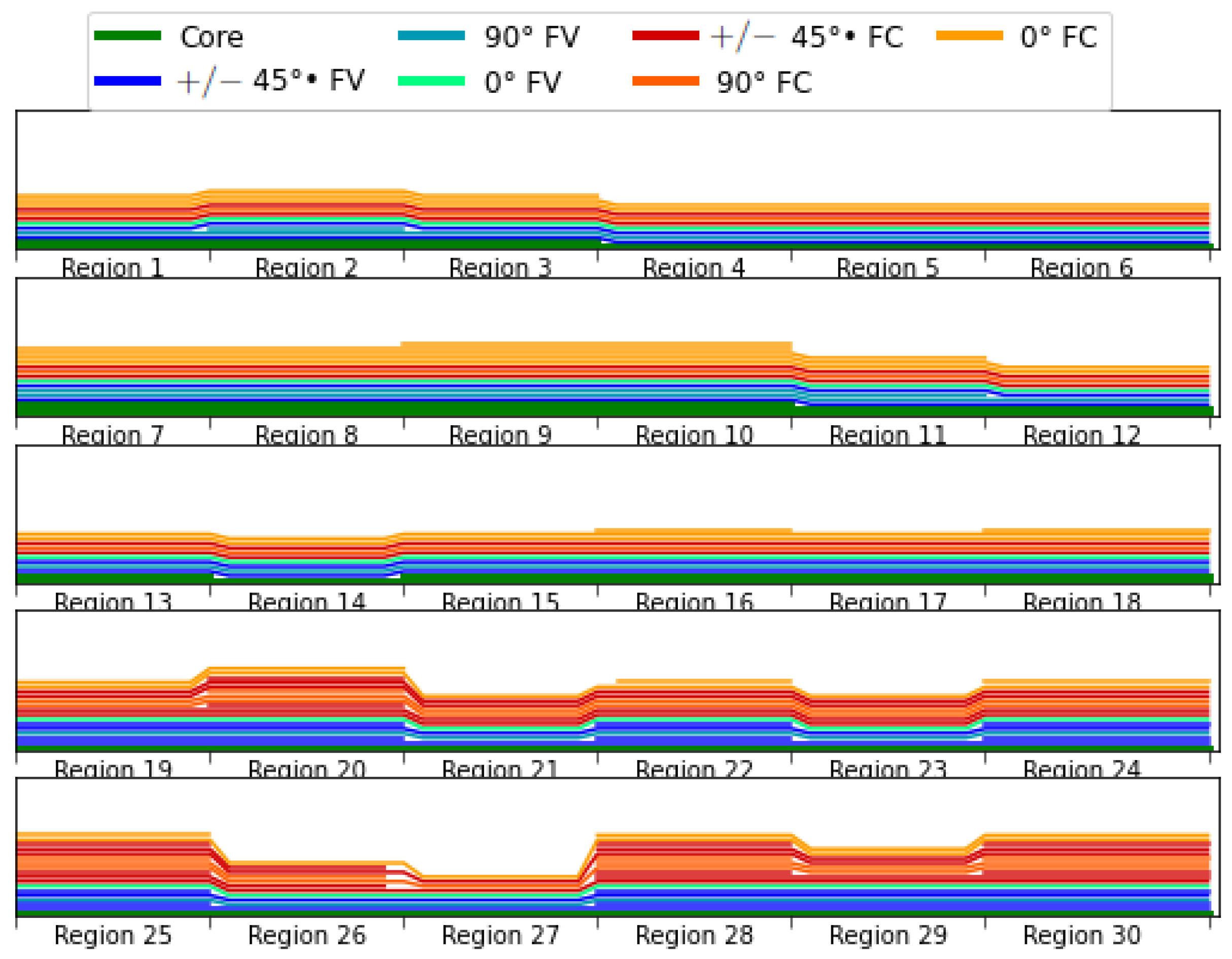
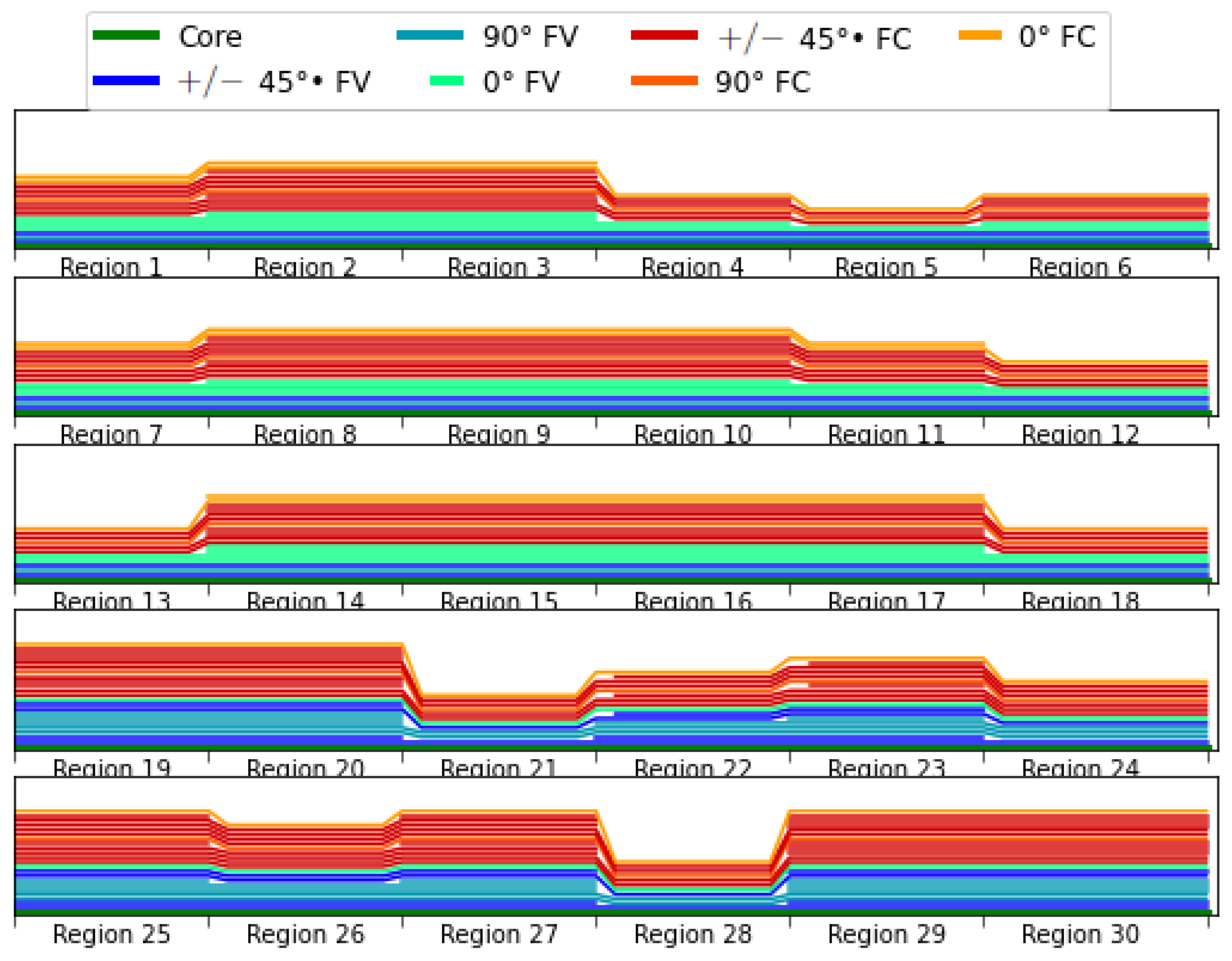
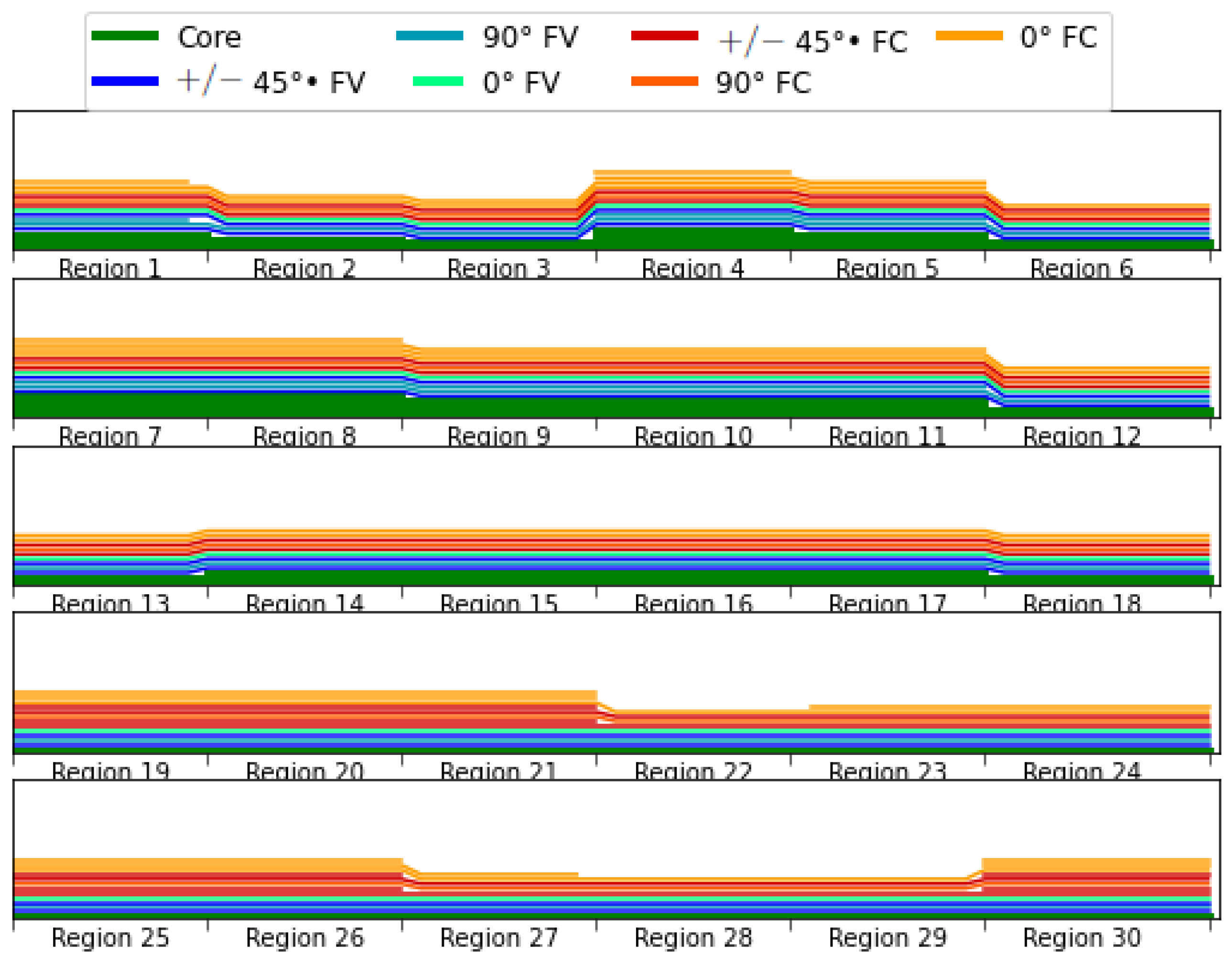
- In the skin regions, the laminates use PVC foam cores, while in the spar regions, no solution has a core. That is because the moment of inertia of the blade in the direction of the main bending loads is heavily increased as the skin thickness gets higher, but is not influenced by the spars’ thickness.
- In all laminates, the overall thickness of the carbon fiber plies is at least double the thickness of the fiberglass. Considering that the fiberglass is heavier and provides less stiffness, that was expected. The values set didn’t allow the number of fiberglass plies to go down to zero. Thus, the fiberglass to carbon fiber ratio could be even lower. However, the blade’s cost is an important industrial design parameter that was not considered in the optimization problem definition. Fiberglass woven is cheaper than carbon fiber and is the main material used in wind turbine blades.
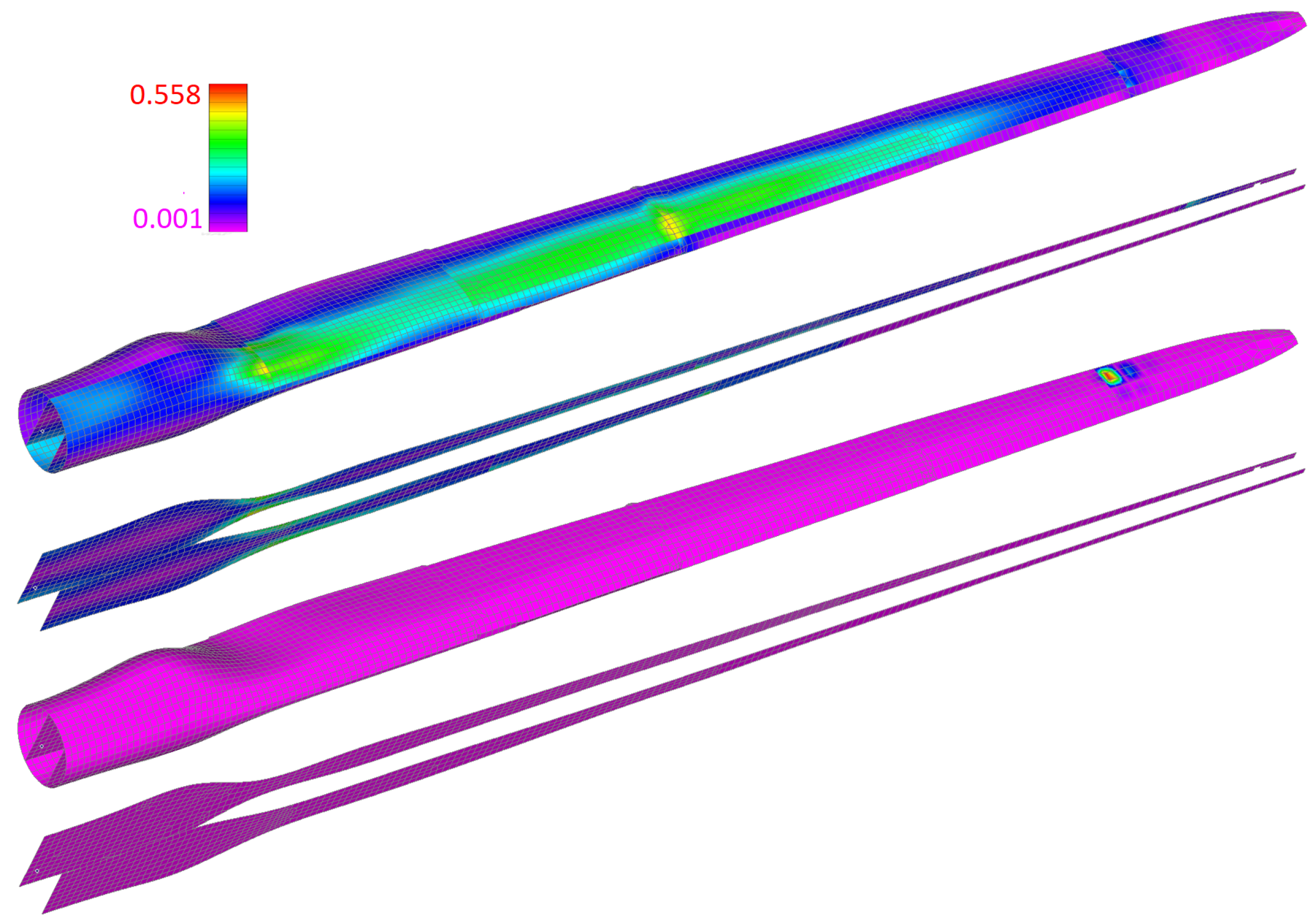
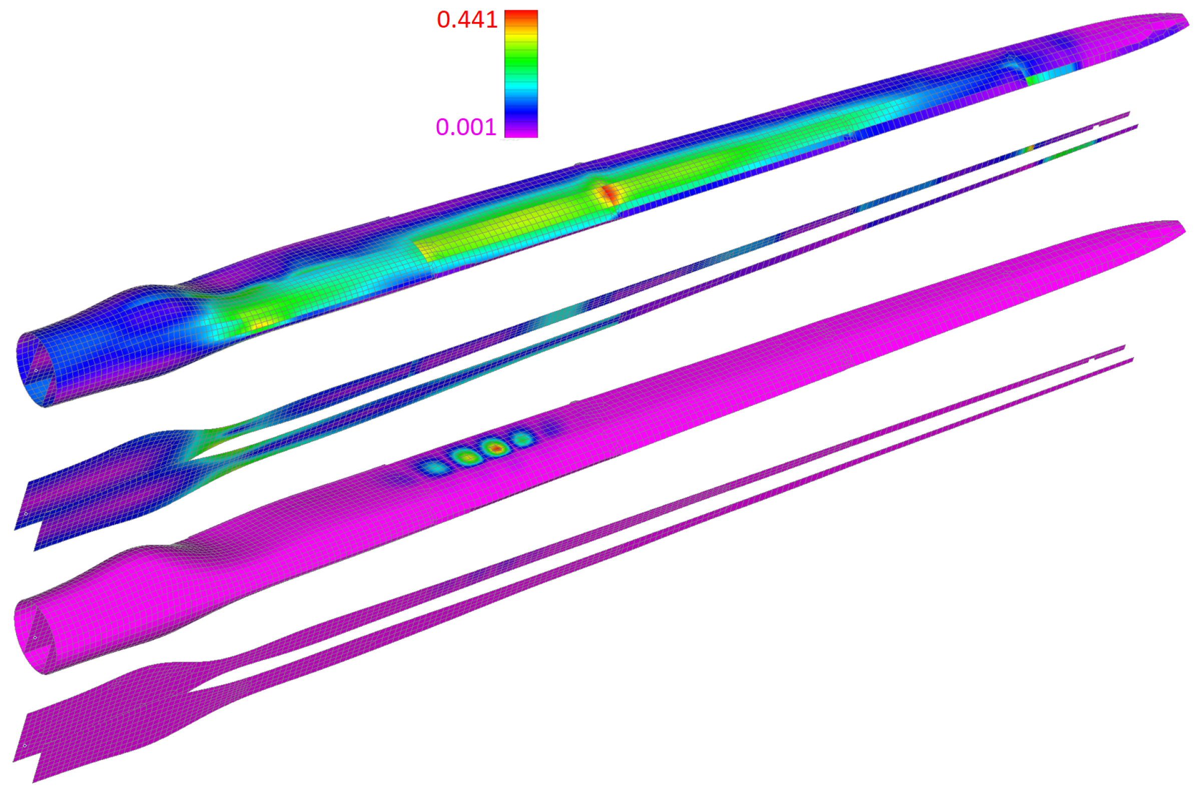
- All solutions observed an unexpected increase in the thickness of the spar regions close to the tip of the blade. The change in the aerodynamic airfoils can explain that behavior through the length of the blade that causes the skin of the blade to be flatter and therefore more prone to local buckling, requiring the spars’ reinforcement. However, it’s also important to add that due to the blade’s tapering, the increase in thickness in those areas causes a minimal increase in weight.
- Through the analysis of results, it can be concluded that adding ply staggering strategies to the laminate parameterization to avoid abrupt changes in stiffness could also provide better results with a better load path through the structure.
6. Conclusions and Extensions
Author Contributions
Funding
Data Availability Statement
Conflicts of Interest
References
- Talarek, K.; Knitter-Piątkowska, A.; Garbowski, T. Wind Parks in Poland—New Challenges and Perspectives. Energies 2022, 15, 7004. [Google Scholar] [CrossRef]
- Chehouri, A.; Younes, R.; Ilinca, A.; Perron, J. Review of performance optimization techniques applied to wind turbines. Appl. Energy 2015, 142, 361–388. [Google Scholar] [CrossRef]
- Chen, J.; Wang, Q.; Shen, W.Z.; Pang, X.; Li, S.; Guo, X. Structural optimization study of composite wind turbine blade. Mater. Des. 2013, 46, 247–255. [Google Scholar] [CrossRef]
- Sjølund, J.; Lund, E. Structural gradient based sizing optimization of wind turbine blades with fixed outer geometry. Compos. Struct. 2018, 203, 725–739. [Google Scholar] [CrossRef] [Green Version]
- Todoroki, A.; Kawakami, Y. Structural design for CF/GF hybrid wind turbine blade using multi-objective genetic algorithm and kriging model response surface method. In Proceedings of the AIAA Infotech@ Aerospace 2007 Conference and Exhibit, Rohnert Park, CA, USA, 7 May–10 May 2007; p. 2890. [Google Scholar]
- Wang, L.; Wang, T.g.; Luo, Y. Improved non-dominated sorting genetic algorithm (NSGA)-II in multi-objective optimization studies of wind turbine blades. Appl. Math. Mech. 2011, 32, 739–748. [Google Scholar] [CrossRef]
- Hu, W.; Han, I.; Park, S.C.; Choi, D.H. Multi-objective structural optimization of a HAWT composite blade based on ultimate limit state analysis. J. Mech. Sci. Technol. 2012, 26, 129–135. [Google Scholar] [CrossRef]
- Dal Monte, A.; Castelli, M.R.; Benini, E. Multi-objective structural optimization of a HAWT composite blade. Compos. Struct. 2013, 106, 362–373. [Google Scholar] [CrossRef]
- Zhu, J.; Cai, X.; Pan, P.; Gu, R. Multi-objective structural optimization design of horizontal-axis wind turbine blades using the non-dominated sorting genetic algorithm II and finite element method. Energies 2014, 7, 988–1002. [Google Scholar] [CrossRef] [Green Version]
- He, Y.; Agarwal, R.K. Shape optimization of NREL S809 airfoil for wind turbine blades using a multiobjective genetic algorithm. Int. J. Aerosp. Eng. 2014, 2014, 864210. [Google Scholar] [CrossRef]
- Durillo, J.J.; Nebro, A.J.; Alba, E. The jMetal framework for multi-objective optimization: Design and architecture. In Proceedings of the IEEE Congress on Evolutionary Computation, Barcelona, Spain, 18–23 July 2010; IEEE: Piscataway, NJ, USA, 2010; pp. 1–8. [Google Scholar]
- Gao, Q.; Cai, X.; Zhu, J.; Guo, X. Multi-objective optimization and fuzzy evaluation of a horizontal axis wind turbine composite blade. J. Renew. Sustain. Energy 2015, 7, 063109. [Google Scholar] [CrossRef]
- Sessarego, M.; Dixon, K.; Rival, D.; Wood, D. A hybrid multi-objective evolutionary algorithm for wind-turbine blade optimization. Eng. Optim. 2015, 47, 1043–1062. [Google Scholar] [CrossRef] [Green Version]
- Fagan, E.M.; De La Torre, O.; Leen, S.B.; Goggins, J. Validation of the multi-objective structural optimisation of a composite wind turbine blade. Compos. Struct. 2018, 204, 567–577. [Google Scholar] [CrossRef]
- Meng, R.; Wang, L.; Cai, X.; Xie, N.g. Multi-objective aerodynamic and structural optimization of a wind turbine blade using a novel adaptive game method. Eng. Optim. 2020, 52, 1441–1460. [Google Scholar] [CrossRef]
- Özkan, R.; Genç, M.S. Multi-objective structural optimization of a wind turbine blade using NSGA-II algorithm and FSI. Aircr. Eng. Aerosp. Technol. 2021, 93, 1029–1042. [Google Scholar] [CrossRef]
- Zhu, J.; Cai, X.; Gu, R. Multi-objective aerodynamic and structural optimization of horizontal-axis wind turbine blades. Energies 2017, 10, 101. [Google Scholar] [CrossRef] [Green Version]
- Zhu, J.; Zhou, Z.; Cai, X. Multi-objective aerodynamic and structural integrated optimization design of wind turbines at the system level through a coupled blade-tower model. Renew. Energy 2020, 150, 523–537. [Google Scholar] [CrossRef]
- Rashedi, A.; Sridhar, I.; Tseng, K. Multi-objective material selection for wind turbine blade and tower: Ashby’s approach. Mater. Des. 2012, 37, 521–532. [Google Scholar] [CrossRef]
- Shen, X.; Chen, J.G.; Zhu, X.C.; Liu, P.Y.; Du, Z.H. Multi-objective optimization of wind turbine blades using lifting surface method. Energy 2015, 90, 1111–1121. [Google Scholar] [CrossRef] [Green Version]
- Wang, L.; Wang, T.; Wu, J.; Chen, G. Multi-objective differential evolution optimization based on uniform decomposition for wind turbine blade design. Energy 2017, 120, 346–361. [Google Scholar] [CrossRef]
- Wang, L.; Han, R.; Wang, T.; Ke, S. Uniform decomposition and positive-gradient differential evolution for multi-objective design of wind turbine blade. Energies 2018, 11, 1262. [Google Scholar] [CrossRef] [Green Version]
- Neto, J.X.V.; Junior, E.J.G.; Moreno, S.R.; Ayala, H.V.H.; Mariani, V.C.; dos Santos Coelho, L. Wind turbine blade geometry design based on multi-objective optimization using metaheuristics. Energy 2018, 162, 645–658. [Google Scholar] [CrossRef]
- Meng, R.; Xie, N.G. A competitive-cooperative game method for multi-objective optimization design of a horizontal axis wind turbine blade. IEEE Access 2019, 7, 155748–155758. [Google Scholar] [CrossRef]
- Zhu, J.; Ni, X.; Shen, X. Aerodynamic and structural optimization of wind turbine blade with static aeroelastic effects. Int. J. Low-Carbon Technol. 2020, 15, 55–64. [Google Scholar] [CrossRef]
- Li, Y.; Wei, K.; Yang, W.; Wang, Q. Improving wind turbine blade based on multi-objective particle swarm optimization. Renew. Energy 2020, 161, 525–542. [Google Scholar] [CrossRef]
- Richardson, J.N.; Adriaenssens, S.; Bouillard, P.; Filomeno Coelho, R. Multiobjective topology optimization of truss structures with kinematic stability repair. Struct. Multidiscip. Optim. 2012, 46, 513–532. [Google Scholar] [CrossRef]
- Carvalho, J.P.G.; Carvalho, É.C.; Vargas, D.E.; Hallak, P.H.; Lima, B.S.; Lemonge, A.C. Multi-objective optimum design of truss structures using differential evolution algorithms. Comput. Struct. 2021, 252, 106544. [Google Scholar] [CrossRef]
- Lemonge, A.C.; Carvalho, J.P.; Hallak, P.H.; Vargas, D.E. Multi-objective truss structural optimization considering natural frequencies of vibration and global stability. Expert Syst. Appl. 2021, 165, 113777. [Google Scholar] [CrossRef]
- Jonkman, J.M.; Hayman, G.; Jonkman, B.; Damiani, R.; Murray, R. AeroDyn v15 User’s Guide and Theory Manual; NREL Draft Report; NREL: Jefferson County, CO, USA, 2015; p. 46. [Google Scholar]
- Zhang, Q.; Li, H. MOEA/D: A multiobjective evolutionary algorithm based on decomposition. IEEE Trans. Evol. Comput. 2007, 11, 712–731. [Google Scholar] [CrossRef]
- Lin, Q.; Li, J.; Du, Z.; Chen, J.; Ming, Z. A novel multi-objective particle swarm optimization with multiple search strategies. Eur. J. Oper. Res. 2015, 247, 732–744. [Google Scholar] [CrossRef]
- Mirjalili, S.; Saremi, S.; Mirjalili, S.M.; Coelho, L.d.S. Multi-objective grey wolf optimizer: A novel algorithm for multi-criterion optimization. Expert Syst. Appl. 2016, 47, 106–119. [Google Scholar] [CrossRef]
- Deb, K.; Pratap, A.; Agarwal, S.; Meyarivan, T. A fast and elitist multiobjective genetic algorithm: NSGA-II. IEEE Trans. Evol. Comput. 2002, 6, 182–197. [Google Scholar] [CrossRef] [Green Version]
- Siemens, A. Simcenter Nastran User’s Guide; Siemens Digital Industry Software Inc.: Plano, TX, USA, 2014. [Google Scholar]
- Van Rossum, G.; Drake, F.L., Jr. Python Reference Manual; Centrum voor Wiskunde en Informatica: Amsterdam, The Netherlands, 1995. [Google Scholar]
- Blank, J.; Deb, K. Pymoo: Multi-Objective Optimization in Python. IEEE Access 2020, 8, 89497–89509. [Google Scholar] [CrossRef]
- Siemens, A. Femap API Reference; Siemens Digital Industry Software Inc.: Plano, TX, USA, 2021. [Google Scholar]
- Höyland, J. Challenges for Large Wind Turbine Blades. Ph.D. Thesis, Norwegian University of Science and Technology, Trondheim, Norway, 2010. [Google Scholar]
- Diab Group. Divinycell H-Technical Data. Available online: https://www.diabgroup.com/products/divinycell-pvc/ (accessed on 15 July 2022).
- Ramachandran, M.; Retnam, B.S.J.; Sivapragash, M.; Raja, D. Analysis of mechanical properties of glass and carbon fiber reinforced polymer material. Int. J. Appl. Eng. Res. 2015, 10, 10387–10391. [Google Scholar]
- Morăraș, C.I.; Goanță, V.; Husaru, D.; Istrate, B.; Bârsănescu, P.D.; Munteanu, C. Analysis of the Effect of Fiber Orientation on Mechanical and Elastic Characteristics at Axial Stresses of GFRP Used in Wind Turbine Blades. Polymers 2023, 15, 861. [Google Scholar] [CrossRef]
- Morăraș, C.I.; Goanță, V.; Istrate, B.; Munteanu, C.; Dobrescu, G.S. Structural Testing by Torsion of Scalable Wind Turbine Blades. Polymers 2022, 14, 3937. [Google Scholar] [CrossRef]
- Bettebghor, D.; Bartoli, N. Approximation of the critical buckling factor for composite panels. Struct. Multidiscip. Optim. 2012, 46, 561–584. [Google Scholar] [CrossRef] [Green Version]
- Bruyneel, M.; Grihon, S.; Sosonkina, M. New approach for the stacking sequence optimization based on continuous topology optimization. In Proceedings of the 8th ASMO UK, ISSMO Conference on Engineering Optimization, London, UK, 8–9 July 2010. [Google Scholar]
- IEC 614001 Ed. 3; Wind Turbines-Part 1: Design Requirements. IEC: Geneva, Switzerland, 2006.
- Bathe, K.J. Finite Element Procedures; Prentice Hall: Upper Saddle River, NJ, USA, 1996. [Google Scholar]
- McGuire, W.; Gallagher, R.H.; Ziemian, R.D. Matrix Structural Analysis, 2nd ed.; John Wiley & Sons: New York, NY, USA, 2014. [Google Scholar]
- Waddoups, M. Advanced Composite Material Mechanics for the Design and Stress Analyst; Fort Worth Division Report FZM-4763; General Dynamics: Fort Worth, TX, USA, 1967. [Google Scholar]
- Griffin, D.A. Blade System Design Studies Volume II: Preliminary Blade Designs and Recommended Test Matrix; Technical Report SAND2004-0073; SANDIA: Albuquerque, NM, USA; Livermore, CA, USA, 2004. [Google Scholar]
- Jonkman, J.; Butterfield, S.; Musial, W.; Scott, G. Definition of a 5-MW Reference wind Turbine for Offshore System Development; Technical Report; National Renewable Energy Lab.(NREL): Golden, CO, USA, 2009. [Google Scholar]
- MacNeal, R.H. The evolution of lower order plate and shell elements in MSC/NASTRAN. Finite Elem. Anal. Des. 1989, 5, 197–222. [Google Scholar] [CrossRef]
- Jonkman, J.; Jonkman, B. NWTC Information Portal (FAST). Available online: https://nwtc.nrel.gov/FAST (accessed on 17 February 2022).
- Audet, C.; Bigeon, J.; Cartier, D.; Le Digabel, S.; Salomon, L. Performance indicators in multiobjective optimization. Eur. J. Oper. Res. 2021, 292, 397–422. [Google Scholar] [CrossRef]
- Zitzler, E.; Deb, K.; Thiele, L. Comparison of multiobjective evolutionary algorithms: Empirical results. Evol. Comput. 2000, 8, 173–195. [Google Scholar] [CrossRef] [Green Version]
- Schott, J.R. Fault Tolerant Design Using Single and Multicriteria Genetic Algorithm Optimization. Ph.D. Thesis, Massachusetts Institute of Technology, Cambridge, MA, USA, 1995. [Google Scholar]
- Tzeng, G.H.; Huang, J.J. Multiple Attribute Decision Making: Methods and Applications; CRC Press: Boca Raton, FL, USA, 2011. [Google Scholar]
- Alkayem, N.F.; Parida, B.; Pal, S. Optimization of friction stir welding process using NSGA-II and DEMO. Neural Comput. Appl. 2019, 31, 947–956. [Google Scholar] [CrossRef]
- Peng, T.; Zhou, J.; Zhang, C.; Sun, N. Modeling and combined application of orthogonal chaotic NSGA-II and improved TOPSIS to optimize a conceptual hydrological model. Water Resour. Manag. 2018, 32, 3781–3799. [Google Scholar] [CrossRef]
- Afzal, A.; Buradi, A.; Jilte, R.; Shaik, S.; Kaladgi, A.R.; Arıcı, M.; Lee, C.T.; Nižetić, S. Optimizing the thermal performance of solar energy devices using meta-heuristic algorithms: A critical review. Renew. Sustain. Energy Rev. 2023, 173, 112903. [Google Scholar] [CrossRef]
- Lara, M.; Garrido, J.; Ruz, M.L.; Vázquez, F. Multi-objective optimization for simultaneously designing active control of tower vibrations and power control in wind turbines. Energy Rep. 2023, 9, 1637–1650. [Google Scholar] [CrossRef]
- Witanowski, Ł.; Klonowicz, P.; Lampart, P.; Ziółkowski, P. Multi-objective optimization of the ORC axial turbine for a waste heat recovery system working in two modes: Cogeneration and condensation. Energy 2023, 264, 126187. [Google Scholar] [CrossRef]
- Deb, K. Multi-Objective Optimization Using Evolutionary Algorithms; John Wiley & Sons, Inc.: New York, NY, USA, 2001. [Google Scholar]
- Li, M.; Zhen, L.; Yao, X. How to read many-objective solution sets in parallel coordinates [educational forum]. IEEE Comput. Intell. Mag. 2017, 12, 88–100. [Google Scholar] [CrossRef]
- Deb, K.; Agrawal, S.; Pratap, A.; Meyarivan, T. A fast elitist non-dominated sorting genetic algorithm for multi-objective optimization: NSGA-II. In Proceedings of the International Conference on Parallel Problem Solving from Nature, Paris, France, 18–20 September 2000; Springer: Berlin/Heidelberg, Germany, 2000; pp. 849–858. [Google Scholar]
- Buljak, V.; Maier, G. Proper orthogonal decomposition and radial basis functions in material characterization based on instrumented indentation. Eng. Struct. 2011, 33, 492–501. [Google Scholar] [CrossRef]
- Márquez, F.P.G.; Chacón, A.M.P. A review of non-destructive testing on wind turbines blades. Renew. Energy 2020, 161, 998–1010. [Google Scholar] [CrossRef]
- Kaewniam, P.; Cao, M.; Alkayem, N.F.; Li, D.; Manoach, E. Recent advances in damage detection of wind turbine blades: A state-of-the-art review. Renew. Sustain. Energy Rev. 2022, 167, 112723. [Google Scholar] [CrossRef]
- Deb, K.; Jain, H. An evolutionary many-objective optimization algorithm using reference-point-based nondominated sorting approach, part I: Solving problems with box constraints. IEEE Trans. Evol. Comput. 2013, 18, 577–601. [Google Scholar] [CrossRef]


| Property | Carbon Fiber UD [39] | Fiberglass UD [39] | Divinycell H200 [40] |
|---|---|---|---|
| (kg/m³) | 1560 | 1890 | 200 |
| (GPa) | 139 | 41 | 0.25 |
| (GPa) | 9 | 9 | 0.25 |
| (GPa) | 5.5 | 4.1 | 0.085 |
| 0.32 | 0.30 | 0.35 | |
| (MPa) | 0.017 | 0.029 | 0.028 |
| (MPa) | −0.007 | −0.020 | 0.019 |
| (MPa) | 0.006 | 0.004 | 0.028 |
| (MPa) | −0.025 | −0.013 | 0.019 |
| (MPa) | 0.013 | 0.022 | 0.041 |
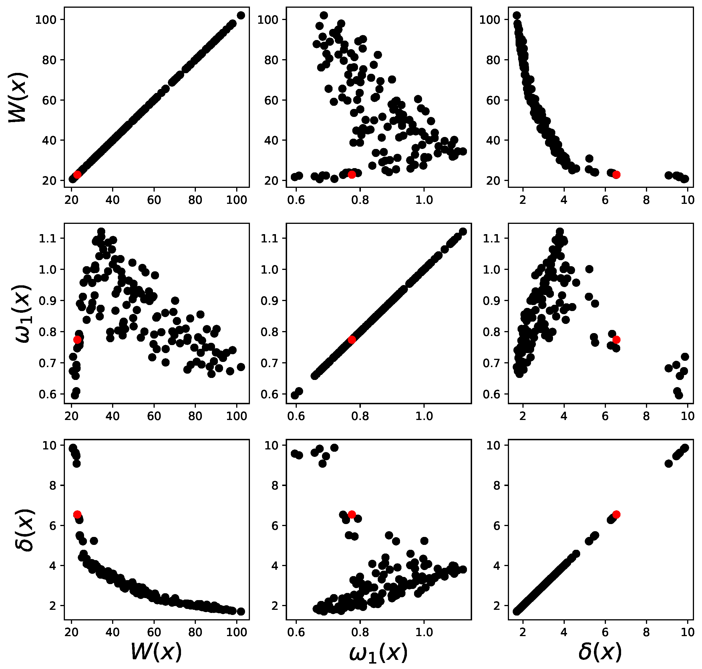
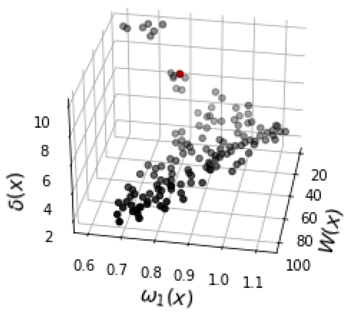
[t] | [Hz] | [Hz] | [Hz] | [m] | |||
|---|---|---|---|---|---|---|---|
| MOSOP1 | 21.90 | 0.965 | 1.392 | 2.720 | 5.69 | 1.27 | 0.754 |
| MOSOP2 | 22.84 | 0.774 | 1.373 | 2.493 | 6.54 | 1.38 | 0.667 |
| MOSOP3 | 36.57 | 0.673 | 1.217 | 2.261 | 6.73 | 1.90 | 0.558 |
| MOSOP4 | 26.29 | 0.859 | 1.701 | 2.855 | 5.05 | 1.44 | 0.441 |
Disclaimer/Publisher’s Note: The statements, opinions and data contained in all publications are solely those of the individual author(s) and contributor(s) and not of MDPI and/or the editor(s). MDPI and/or the editor(s) disclaim responsibility for any injury to people or property resulting from any ideas, methods, instructions or products referred to in the content. |
© 2023 by the authors. Licensee MDPI, Basel, Switzerland. This article is an open access article distributed under the terms and conditions of the Creative Commons Attribution (CC BY) license (https://creativecommons.org/licenses/by/4.0/).
Share and Cite
Couto, L.d.L.; Moreira, N.E.; Saito, J.Y.d.O.; Hallak, P.H.; Lemonge, A.C.d.C. Multi-Objective Structural Optimization of a Composite Wind Turbine Blade Considering Natural Frequencies of Vibration and Global Stability. Energies 2023, 16, 3363. https://doi.org/10.3390/en16083363
Couto LdL, Moreira NE, Saito JYdO, Hallak PH, Lemonge ACdC. Multi-Objective Structural Optimization of a Composite Wind Turbine Blade Considering Natural Frequencies of Vibration and Global Stability. Energies. 2023; 16(8):3363. https://doi.org/10.3390/en16083363
Chicago/Turabian StyleCouto, Lucas de Landa, Nícolas Estanislau Moreira, Josué Yoshikazu de Oliveira Saito, Patricia Habib Hallak, and Afonso Celso de Castro Lemonge. 2023. "Multi-Objective Structural Optimization of a Composite Wind Turbine Blade Considering Natural Frequencies of Vibration and Global Stability" Energies 16, no. 8: 3363. https://doi.org/10.3390/en16083363