A Review of Reinforcement Learning-Based Powertrain Controllers: Effects of Agent Selection for Mixed-Continuity Control and Reward Formulation

Abstract

One major cost of improving the automotive fuel economy while simultaneously reducing tailpipe emissions is increased powertrain complexity. This complexity has consequently increased the resources (both time and money) needed to develop such powertrains. Powertrain performance is heavily influenced by the quality of the controller/calibration. Since traditional control development processes are becoming resource-intensive, better alternate methods are worth pursuing. Recently, reinforcement learning (RL), a machine learning technique, has proven capable of creating optimal controllers for complex systems. The model-free nature of RL has the potential to streamline the control development process, possibly reducing the time and money required. This article reviews the impact of choices in two areas on the performance of RL-based powertrain controllers to provide a better awareness of their benefits and consequences. First, we examine how RL algorithm action continuities and control–actuator continuities are matched, via native operation or conversion. Secondly, we discuss the formulation of the reward function. RL is able to optimize control policies defined by a wide spectrum of reward functions, including some functions that are difficult to implement with other techniques. RL action and control–actuator continuity matching affects the ability of the RL-based controller to understand and operate the powertrain while the reward function defines optimal behavior. Finally, opportunities for future RL-based powertrain control development are identified and discussed.

1. Introduction

Over the years, rising fuel economy standards and required reductions in greenhouse gas emissions have necessitated increases in powertrain complexity. Increases in powertrain complexity come in the form of additional actuators and control systems within the internal combustion engines (ICE) and/or the addition of various electrification methods within the powertrain. Recently, powertrain electrification has been a popular choice to tackle the increase in vehicle operating standards. Powertrain electrification allows for capturing otherwise waste energy within the powertrain and the ability to improve vehicle performance using technologies such as four-wheel independent drive (4WID). The exact amount of electrification varies vehicle to vehicle, and includes solutions such as battery electric vehicles (BEVs), fuel cell vehicles (FCVs), and hybrid electric vehicles (HEVs). Similarly to ICE powertrains, BEVs and FCVs are powered by a single power source, a battery, and a fuel cell, respectively. Hybrid vehicles include any powertrain that contains multiple energy storage mechanisms. These sources can be any combination of batteries, ultracapicators, ICEs, fuel cells, and/or waste energy recovery systems with the exact combination varying application to application. The added powertrain complexity significantly increases the effort needed to calibrate control systems. Many recent studies utilize reinforcement learning (RL) for powertrain control applications, seeking to improve vehicle performance or reduce calibration efforts. This manuscript summarizes the existing literature and provides a review of two critical aspects of RL-based powertrain control: agent selection and reward function formulation.

Control techniques used within the automotive industry can be broken down into rule-based and optimization-based categories, a selection of which are shown in Figure 1. Optimization-based control techniques are rooted in optimal control theory and utilize an optimizer to exploit information about the controlled system to schedule control actions that minimize/maximize expected returns as defined by a cost/reward function.

Classically, powertrain controllers have been developed using rule-based techniques. Rule-based techniques are well-suited for control of actuators with mixed continuities as rules can be written in discrete and continuous domains. Furthermore, rules can be written case by case to ensure adherence to regulatory requirements while maintaining high performance. However, rule-based methods are poorly equipped to handle the non-linear complexity increases associated with emerging powertrain configurations. Adding any technology to a powertrain exponentially increases the calibration effort needed to obtain the reductions in fuel economy each technology promises [1]. Beyond a specific complexity level, rule-based techniques driven by calibrated tables [2,3] break down. The exponential increase in computing requirements from the growth of the design space is called the curse of dimensionality [4]. This curse is an active limitation in powertrain development and is especially present as the powertrain is hybridized [5]. Intelligent design of experiment processes [6,7] and machine learning [8] have been used to reduce the calibration burden of rule-based control techniques, but these only temporarily mitigate the curse of dimensionality rather than eliminate it. The challenge to produce a standards-compliant powertrain subject to the time and financial pressures within the automotive industry has resulted in the investigation of optimization-based control techniques.

Optimal control of modern powertrains is challenging for several reasons, as powertrains:

• Are highly complex nonlinear systems. This makes representative powertrain models difficult to derive and computationally heavy.
• Contain a mixture of continuous and discrete actuators. Simultaneous operation in both continuity domains is difficult for many techniques.
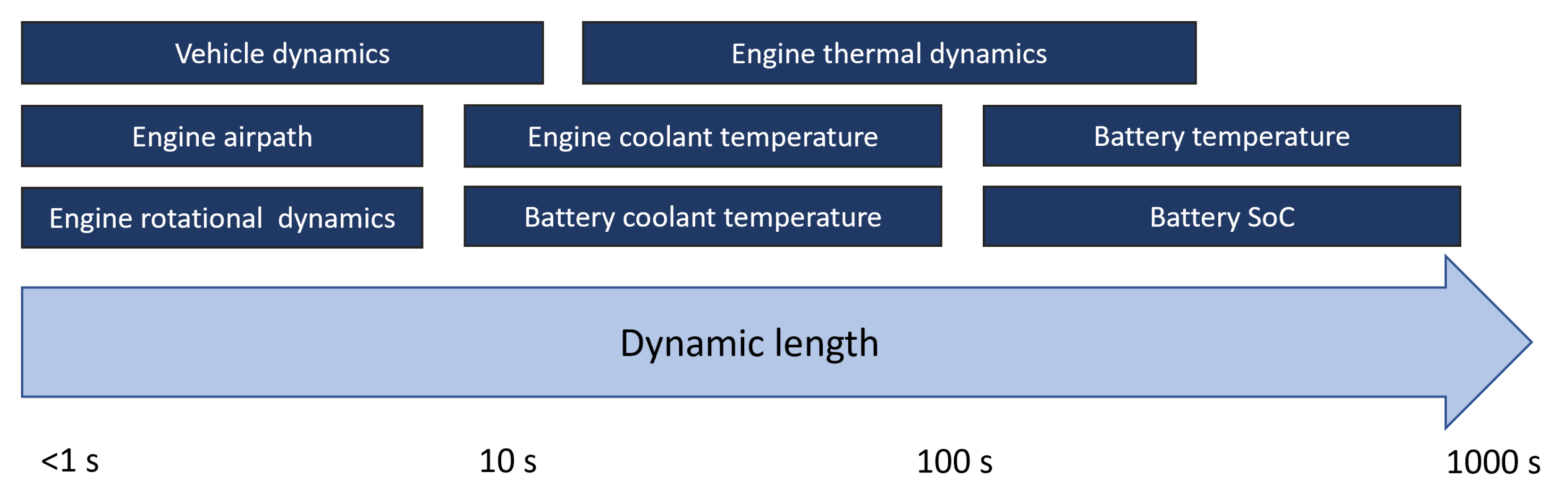
• Have dynamics with timescales orders of magnitudes apart. Controlling a system with mixed timescales requires a small time step and long optimization horizon.
• Performance goals often conflict with regulatory requirements. Defining the control problem mathematically can be difficult.

Optimization-based control covers a wide breadth of techniques and can be split into global and real-time categories, with their ability to address the challenges of modern powertrain control differing by technique. Global techniques attempt to optimize the performance of a system over scenarios of finite length. Real-time techniques are methods that can run online, optimizing performance over a single time step or receding horizon. Dynamic programming is a constrained model-based optimization technique guaranteed to find the global optimal policy over a finite deterministic trajectory. This allows DP to address the challenges of optimizing the performance of systems with a mixture of fast and slow dynamics. However, the curse of dimensionality requires DP to use reduced-order models with a small number of states and control actions. Consequently, insight gained from DP studies must consider the implications of simplifying dynamics to levels tractable by DP as oversimplification can produce subpar real-world performance [9].

ECMS and MPC are real-time optimization techniques capable of functioning in deployed systems. Both techniques rely on a control-oriented model (COM) to derive the optimal control policy which allows them to control systems with higher complexity than DP. ECMS optimizes performance over the next time step while MPC optimizes performance over a receding horizon. As MPC must use the COM during operation, the COM’s computational tractability limits the length of MPC’s receding horizon [10]. This is undesirable because using a complex model to capture all relevant dynamics can restrict the length of the receding horizon to a point where MPC may not be able to optimize all of the desired dynamics directly. While methods to increase the computational tractability of COMs used by MPC have been proposed [11,12,13], they do not address the need of MPC to model system performance at every time step in the receding horizon. Thus, MPC can be formulated to address control of complex systems over short receding horizons or simple systems over long horizons, but not both at once.

Reinforcement learning [14] is an emerging technique that can address the identified challenges in powertrain control. Figure 2 illustrates the development process of a RL-based powertrain control system. RL operates forward in time using trial and error and past experiences to improve their understanding of the value of a given state and/or action [15]. Learning from experiences bypasses the need for RL agents to understand the underlying dynamics of the environment. This allows the environment to have unlimited complexity. Thus, the environment can be a physical system, a virtual prototype/digital twin, or a reduced-order model which directly addresses the challenge of powertrain complexity.Some papers utilize higher-fidelity simulation models as the virtual “vehicle” to capture complex component behaviors such as battery degradation [16,17,18] Since RL has this model-independent nature, this literature review does not focus on exact vehicle and powertrain plant models.

Because RL uses the same underlying principles as DP, it can optimize the performance of systems containing fast and slow dynamics. Prioritization between future rewards and immediate rewards is controlled using a discount factor, $\left\{\gamma |0\le \gamma \le 1\right\}$. Selecting $\gamma =1$ equally distributes emphasis between the present reward and every reward from all future steps. This is akin to the reward formulation used within dynamic programming. Similarly to dynamic programming, when using $\gamma =1$, the number of steps that are optimized over must be finite to allow for a solution to exist. Typically, the optimization goal for a powertrain controller is over the vehicle’s entire lifetime so $\gamma$ must be set to a number less than one. Setting $\gamma <1$ also allows RL to handle stochastic environments which is necessary for online control as real-world operation is not deterministic. To take advantage of RL’s ability to consider long-term dynamics, $\gamma$ is typically selected to be close to one, $\gamma \approx 0.99$, which allows RL to address the second identified challenge of powertrain control development.

Some existing literature provides a general review of utilizing RL for automotive powertrain control [19,20]. While these works demonstrate that it is relatively straightforward to address the first two challenges identified in powertrain control development, addressing the challenges of controlling actuators with a mixture of continuities and reward function formulation is less straightforward and must be handled on a problem-by-problem basis. Making informed decisions in these areas is important as they influence the derived control policy’s optimality. Critically, the magnitude of their influence depends on how sensitive the system being studied is to these decisions in these areas. Presently, there is no powertrain-relevant benchmark commonly used to understand how decisions made compare to decisions made by others across the field. Instead, comparisons made within studies use reference controllers that the authors also develop. The lack of a consistent baseline across studies prevents the relative benefit of a decision from being understood, inhibiting the progress of RL-based powertrain control solutions. The next best option is to review prior RL-based powertrain control studies and examine them holistically to form conclusions. This review is focused on RL-based controllers used within the powertrain to optimize its local performance.

This area of investigation is chosen as local powertrain control has extensive prior research devoted to addressing the third and forth challenges across a full spectrum of control techniques. Critically, decisions to address these challenges influence performance as they define the structure of the optimization problem an agent is tasked to solve. Consequently, examining an algorithm’s ability to learn and how it compares to other algorithms is outside the scope of this review but has been examined by others [14,21,22,23,24]. Additionally, RL is actively being investigated for use in areas of vehicle development such as connected vehicles [25] and fog computing [26]. These new technologies enable functionalities such as transfer learning [27,28,29,30], distributed computation [31], and previewed traffic conditions [32,33]. These topics are beyond the scope of this study. However, the conclusion of this paper regarding the agent selection and reward function formulation can be transferred to the powertrain control of connected vehicles.

The research methodology for this review is outlined as follows: first, RL-based powertrain control studies are identified and divided based on how they address the mixed-continuity control and reward function formulation challenges. The matches between actuator and action continuity we have identified and examined are the control of continuous actuator(s) with discrete action(s), control of continuous actuator(s) with continuous output(s), and the combined control of continuous and discrete actuators. This matching is rarely the primary subject of the study, and thus must be identified during reading. However, studies that compare RL algorithms with differing continuities often mention discrete or continuous continuity in the study’s title. Next, the studies are reorganized to focus on how powertrain optimization goals and constraints have been expressed as reward functions. Goals are identified as single- or multi-objective and further grouped by their specific objectives. The exact objective often appears in the title of the study of single-objective studies while multi-objective studies will either label themselves as such or state all their objectives in the title. Single objectives include the minimization of fuel consumption, power consumption, energy losses, operation cost, tracking error, and maximization of extracted power. Multi-objective approaches can be identified when the author acknowledges there is more than one goal to be considered and that final trade-offs in performance are subject to the designer’s performance. By examining the identified studies using these two lenses, a holistic understanding of decisions being made and their influence on controller performance is formed, and recommendations for future research are provided.

2. Reinforcement Learning Algorithm Selection

Reinforcement learning is an umbrella that covers many algorithms, each with its own advantages and disadvantages. The purpose of this section is to examine factors beyond an algorithm’s ability to learn that influence achieved performance. In particular, consideration must go into pairing an RL algorithm with the associated control challenge. One of the key characteristics of an RL algorithm is the continuity of the actions it takes. Some algorithms can only make discrete actions, others are limited to continuous actions, while some can operate in a combined continuous–discrete action space. A selection of RL algorithms and their action continuities are shown in

Table 1. Action space domains of selected RL algorithms ${}^{†}$.

Algorithm/Agent	Action Space Continuity
Q-learning (table-based) [34]	discrete
Deep Q-network (DQN) [35]	discrete
SARSA [36]	discrete
Policy gradient [37]	discrete or continuous
Proximal policy optimization (PPO) [38]	discrete or continuous
Deep deterministic policy gradient (DDPG) [39]	continuous
Twin delayed DDPG (TD3) [40]	continuous
Maximum a posteriori policy optimization (MPO) [41]	discrete, continuous, or both
Constrained policy optimization (CPO) [42]	discrete, continuous

${}^{†}$ The algorithms above do not form an exhaustive list as many variations on each technique exist and new RL algorithms are actively being proposed.

. Powertrain control can require the scheduling of continuous and discrete signals, examples of which are shown in

Table 2. Example signals that a powertrain controller could be expected to schedule.

Continuous Powertrain Actuators	Discrete Powertrain Actuators
$position$	$gea{r}_{number}$
$velocity$	$clutc{h}_{on/off}$
$power$	$engin{e}_{on/off}$
$power$	$\Delta signa{l}_{discrete}$
$torque$
$flow$
$current$
$\Delta signa{l}_{continuous}$

. A summary of RL algorithms, systems they are applied to, and continuities of both the RL algorithm and system being controlled for the studies identified in this review are shown in

Table 3. Reward functions used in single objective RL-based powertrain control studies.

Optimization Goal	Instantaneous Reward Function	Constraint(s) in Reward Function ${}^{†}$	System Controlled
minimize fuel consumption	$-{\dot{m}}_{fuel}$		parallel [43,44,45], power-split [46] HEV
	${\dot{m}}_{fuel,engineonly}-{\dot{m}}_{fuel,actual}-\mathbf{TC}$		parallel HEV [47,48]
	$-{\dot{m}}_{fuel}-{\dot{m}}_{e.fuel,electrical}$		parallel [49,50,51], series [52], power-split [53] HEV
	$-{\dot{m}}_{fuel}-w_1\dot{SoC}$		parallel HEV [54]
	$-{\dot{m}}_{fuel}-w_1\left|\delta SoC\right|$		series HEV [55]
	$-{\dot{m}}_{fuel}-w_1\delta So{C}^2$		series [56,57,58,59,60,61,62], power-split [63,64,65] HEV
	$-{\dot{m}}_{fuel}-w_1\delta So{C}^2$	$SoC$	power-split [66], series [67] HEV
	$-{\dot{m}}_{fuel}-w_1\delta So{C}^2$	$actionfeasibility$	power-split HEV [68]
	$-{\dot{m}}_{fuel}+w_1{\left[\delta So{C}^2\right]}^{-}$		series [69], parallel [70], power-split [71] HEV
	$\begin{array}{cc}& -{\dot{m}}_{fuel}-w_1\delta So{C}^2·\hfill \\ \hfill & \hfill (SoC<So{C}_{low}\cup So{C}_{high}<SoC)\hfill \end{array}$		parallel [72], power-split [73] HEV
	$-{\dot{m}}_{fuel}-{\dot{m}}_{e.fuel,electrical}-w_1\left|\delta SOC\right|$		parallel HEV [74,75]
	$-{\dot{m}}_{fuel}-{\dot{m}}_{e.fuel,electrical}+w_1{\left[\delta So{C}^2\right]}^{-}$		parallel HEV [76,77]
	$1-(w_1{\dot{m}}_{fuel}+w_2{\dot{m}}_{e.fuel,electrical})$		series HEV [78]
	$-tanh(w_1{\dot{m}}_{fuel}+w_2|\delta SoC\left|\right)$		series HEV [79]
	$-({\dot{m}}_{fuel}+w_1\delta So{C}^2)+w_2{\eta }_{engine}$	${\omega }_{transmission}$	parallel HEV [80]
	$-{\dot{m}}_{fuel}-w_1\delta So{C}^2-w_2\Delta engin{e}_{on/off}$	$SoC$	parallel HEV [81,82]
minimize power consumption	$SoC$		8 × 8 EV [83]
	$-P_{bat}-\mathbf{TC}$		EV with UC and battery [84]
	$\left\{\begin{array}{cc}\frac{1}{P_{engine}},\hfill & \mathrm{if}{P}_{engine}\ne 0\hfill \\ \frac{2}{Mi{n}_{P_{engine}}},\hfill & \hfill \mathrm{otherwise}.\hfill \end{array}\right.$	$SoC$	power-split PHEV  [85,86,87,88]
	$-{\dot{E}}_{fuel}-{\dot{E}}_{electrical}$		parallel HEV [89,90]
	$\begin{array}{cc}\hfill c_1& - (P_{engine}/{\eta }_{engine}-P_{ORC}/{\eta }_{engine}\hfill \\ \hfill & +P_{bat}{{\eta }_{bat}}^{sign\left(P_{bat}\right)})\hfill \\ \hfill & -w_1\Delta engin{e}_{on/off}\hfill \end{array}$	$SoC$	parallel HEV with ORC-WHR [91]
minimize losses	$\begin{array}{cc}\hfill c_1& \hfill - Los{s}_{engine}-Los{s}_{bat}+w_1{\left[\delta SoC\right]}^{-}\hfill \end{array}$		series HEV [92,93]
	$-Los{s}_{bat}-Los{s}_{UC}-Los{s}_{DC/DC}$		EV with UC and battery [94,95]
maximize extracted power	$-P_{turbine}+P_{pump}$		ORC-WHR [96]
minimize cost to operate vehicle	$-{\dot{m}}_{fuel}·pric{e}_{fuel}-\dot{SoC}·pric{e}_{electricity}$		power-split PHEV  [97,98,99]
	$\begin{array}{cc}\hfill -& \hfill {\dot{m}}_{fuel}·pric{e}_{fuel}-\dot{SoC}·pric{e}_{electricity}\hfill \\ \hfill & -w_1\left|\delta SoC\right|\hfill \end{array}$		series PHEV [100]
	$-P_{charge/discharge}·pric{e}_{electricity}$	$SoC·(t\equiv t_{disconnect})$	EV [101]
	$\begin{array}{cc}& -P_{charge/discharge}·pric{e}_{electricity}\\ \hfill & -cos{t}_{degradation,bat}\hfill \\ \hfill & \hfill -w_1\delta So{C}^2·(t\equiv t_{disconnect})\hfill \end{array}$		EV [102]
	$-{\dot{m}}_{fuel}-w_{1}cos{t}_{degradation,bat}$		parallel HEV [18]
minimize tracking error	$-k\delta T,k:=f\left(\delta T\right)$	$\delta T$	ORC-WHR [103]
	$-\delta v$	$\delta v$	bicycle with electric motor [104]

^† Constraints are only listed if they are explicitly listed in the reward function formulation by the author. TC indicates the existence of a terminal reward within the reward function. $\delta X:=\left(X -X_{\mathit{user} \mathit{defined} \mathit{target}}\right)$, $X^{+}:=\max \left(0,X\right)$, $X^{-}:=\min \left(0,X\right)$.

.

If the continuity of the RL algorithm and the signals it is scheduling do not match, a continuity conversion must be performed. Examples of how continuity conversions can be implemented are shown in Figure 3. Performing a continuity conversion reduces the RL-based controller’s performance as it no longer interacts with the environment in its native form. Using a continuous signal to control a discrete actuator results in approximation error as the continuous signal must approximate a discontinuous function, see Figure 4a. Likewise, using a discrete signal to control a continuous actuator is prone to resolution issues as the discrete signal cannot schedule action values finer than the level of discretization implemented, resulting in suboptimal scheduling of the continuous actuator, see Figure 4b.

2.1. Control of Continuous Actuator(s) with Discrete Action Output(s)

When a discrete output is used to control a continuous signal, a discrete-to-continuous conversion must be performed. This conversion is commonly known as discretization, and can be performed in various ways. Two different methods to perform this continuity conversion are used by the studies identified in

Table 4. RL-based powertrain control studies, the action continuity of their chosen RL algorithm(s), and the native continuity of the actuator(s) being controlled.

RL Algorithm(s)	Study	System Controlled	Control Action(s)	Action Continuity	Actuator Continuity
Value estimation	[106]	parallel PHEV	${\tau }_{engine},n_{gear}$	discrete	combined
SARSA	[107]	FC PHEV	$P_{FC}$, weight of penalty on $P_{bat}$	discrete	continuous
Q-learning (table-based)	[49,50,51,70,76,77,81,82]	parallel HEV	$P_x(x=EM\mathrm{or}engine)$	discrete	continuous
	[46,71,85,86,108,109]	power-split HEV	$P_{bat}$
	[66]	power-split HEV	${\tau }_{engine},{\omega }_{engine}$
	[52,56,57,58,59,67,69,78,92]	series HEV	$P_{engine}$
	[84,94,95]	battery-UC EV	$i_{bat}$
	[17]	battery-UC EV	$P_{bat}$
	[105]	FC HEV	$\Delta P_{bat}$
	[110]	FC-battery-UC HEV	$P_{bat},P_{FC}$
	[111]	FC HEV	$So{C}_{min},So{C}_{max}$
	[112]	EV	${\tau }_{EM}$
	[96]	ORC-WHR	${\dot{m}}_{workingfluid}$
	[18,43]	parallel HEV	$i_{bat},n_{gear}$	discrete	combined
Dyna-Q	[52,59,60]	series HEV	$P_{engine}$	discrete	continuous
	[53]	power-split PHEV	$n_{operatingmode}$
Q-learning (approximate)	[54]	parallel HEV	${\tau }_{EM}$	discrete	continuous
	[113]	EV	$\Delta SoC$ overnight
Q-learning vs. DQN	[114]	EV with two batteries	$P_{split}$	discrete	continuous
DQN	[72,91,115,116]	parallel HEV	${\tau }_{engine}$	discrete	continuous
	[63,73,87]	power-split HEV	$\Delta P_{engine}$
	[117]	power-split PHEV	${\tau }_{engine},{\omega }_{engine}$
	[61,100]	series HEV	$po{s}_{throttle}$
	[102]	EV	$i_{charge/discharge}$
	[118]	EV thermal management	${\omega }_{fan},{\omega }_{compressor}$
	[44,45]	parallel HEV	$P_{EM},n_{gear}$	discrete	combined
Double-DQN	[55,62,93,119]	FC series HEV	$\Delta P_{FC}$	discrete	continuous
	[120]	vehicle	$po{s}_{pedal}$
Dueling-DQN	[88]	power-split PHEV	$P_{engine}$	discrete	continuous
Double-DQN and DDPG	[80]	parallel HEV	$po{s}_{throttle},n_{gear}$	combined	combined
DDPG	[72,75,89,121]	parallel HEV	$P_{EM}$	continuous	continuous
	[47,48,90]	parallel HEV	$P_{EM},coo{l}_{battery}$
	[79]	series HEV	$\Delta P_{engine}$
	[65]	power-split HEV	$P_{engine}$
	[103]	ORC-WHR	${\omega }_{pump}$
	[83]	8 × 8 EV	${\tau }_{wheel,x}$
	[73,97]	power-split HEV	${\tau }_{engine},{\omega }_{engine},{\tau }_{EM}$
	[64]	power-split HEV	$n_{operatingmode},{\tau }_{engine},$ ${\omega }_{engine}$	continuous	combined
TD3	[72,74,75]	parallel HEV	$P_{split}$	continuous	continuous
	[122]	parallel HEV	${\tau }_{engine}$
actor-critic	[99]	power-split PHEV	${\tau }_{engine},{\omega }_{engine},P_{split}$	continuous	continuous
	[123]	vehicle	$\dot{v}$
	[124]	SI engine	${\dot{m}}_{air}$
	[98]	power-split PHEV	${\tau }_{engine},{\omega }_{engine},$ ${\tau }_{EM},clutc{h}_{on/off}$	combined	combined
actor-critic (two actors)	[125]	series hydraulic hybrid	${\tau }_{engine},{\omega }_{engine}$	continuous	continuous
	[126]	vehicle	$\Delta gear$ (discrete), $P_{traction}$ (continuous)	combined	combined
PPO	[127]	parallel HEV	${\tau }_{engine},{\omega }_{engine},{\tau }_{traction}$	continuous	continuous
CPO	[101]	EV	$i_{charge/discharge}$	discrete	continuous
A3C	[68]	power-split HEV	${\tau }_{engine},{\omega }_{engine},$	either	continuous

. The first method, Figure 5a, is to discretize the range of the continuous action directly and is the most common approach used by the RL-based powertrain control studies identified. The second method, Figure 5b, defines the RL agent output as the desired change ($\Delta$) of the continuous signal from the previous time step to the current. When using the second method, the number of outputs for the RL agent has to be at least three: increase, decrease, and hold. Reddy et al. [105] used the minimum quantity when developing a Q-learning-based energy management strategy (EMS) for a fuel cell hybrid vehicle, though more than three outputs are commonly used as it gives the RL agent greater control authority. For action spaces with more than three outputs, it can be beneficial to use non-uniform steps. Wu et al. [63] controlled the engine power of a power-split HEV with outputs of $\Delta P_{engine}=\{-1,0,+1,+20,+40,set0\}$ for their DQN-based EMS. Neither discretization method is better than the other, as both have limitations. The first method is limited by the level of resolution used for discretization as too fine a resolution will result in a computationally infeasible number of discrete output values. As stated previously, the second method can operate using as few as three discrete outputs. However, the second method requires that the previous value of the controlled signal is passed to the agent as a state. For RL algorithms that must discretize the state space of the environment, the second method does not guarantee a decrease in the number of values being tracked. In addition, a RL agent using the second method is not guaranteed in its ability to reach any continuous action output from any previous value, which reduces the control authority of the RL agent.

A benefit of using discrete action outputs to control continuous actuators is that the designer has more control over the action space. Biswas et al. [68] demonstrated that the intelligent design of the discrete action space increased beneficial exploration of the operating space compared to using a continuous action space. Their RL agent controlled engine speed and torque for a power–split hybrid.With this powertrain, these two actions cannot be selected independently as engine torque cannot be greater than zero if the engine is not rotating. They pruned the discrete action space only to contain feasible combinations of these two actions. They found that using the pruned discrete action space led to more reliable convergence and higher performance policies than using continuous action outputs where the infeasible set of control action combinations was not removed.

The penalty of using a discrete-to-continuous continuity conversion has been well documented in both RL and non-RL literature. While studying the use of Q-learning as a parallel HEV EMS, Xu et al. [49] showed that the optimality of the RL agent depends on the resolution of the discretization used, Figure 6. The performance of the Q-learning agent examined by Xu et al. asymptotically approaches a limit as the level of discretization increases. This indicates that the higher the discretization level, the more the output behaves like a continuous output, and the better the agent performs. In addition to the optimality loss induced by performing a discrete-to-continuous continuity conversion, its existence also increases the resources needed since an additional hyperparameter, the level of discretization per signal, must be tuned by the designer. Always using high levels of discretization to avoid a penalty for using a continuity conversion is not a practical solution. Each additional actuator controlled increases the number of discrete action combinations exponentially exposing the approach to the curse of dimensionality. Therefore, like DP, there is a limit to the number of actuators RL algorithms with discrete outputs can control. Of the studies identified in this review, no RL agent that utilizes a discrete-to-continuous continuity conversion controls more than two actions.

Despite the limitations, many RL agents with discrete-to-continuous continuity conversions have been developed as RL-based powertrain controllers. Just under three-quarters of the RL-based powertrain studies identified in Table 4 control a continuous actuator via a discrete action output. Of these studies, the majority focus on RL-based EMS for hybrid vehicles, while others examine eco-focused velocity control [112,120], grid-to-EV charging [102,113], and control of an organic Rankine cycle-waste heat-recovery system [96].

RL-based EMS is a popular topic of study as its challenges are well-matched to RL’s strengths. The primary job of an EMS is to govern how the vehicle’s power demand is split among multiple power sources. At any given time, an EMS must decide how much of the vehicle power request is met by each power source. Meeting the vehicle power request mostly with one power source can improve instantaneous efficiency. However, doing so reduces the amount of energy available from the power source that can be used to meet future demands. When a battery is used as a power source it can have charging dynamics that are orders of magnitude slower than the timescale power split decisions must be made. The uncertainty in future power demands and slow battery dynamics make EMS control a long-term optimization problem, which RL is well-suited to handle. The model-free nature of many RL algorithms further strengthens RL’s appeal as vehicle efficiency is the product of the interactions of many sub-systems and components.

Despite power-split being a continuous control action, many researchers have successfully trained RL-based EMS using agents with discrete action outputs to determine power-split. While reported performance improvement is highly dependent on the quality of the baseline controller RL is compared to, RL has compared favorably to ECMS [74], MPC [76], SDP [81], and rule-based EMS [78] despite the optimality loss associated with a discrete-to-continuous continuity conversion. However, as RL-based powertrain control matures it will be tasked with governing systems with greater control complexity, increasing the risk that the curse of dimensionality will prohibit the use of RL algorithms limited to discrete action outputs.

2.2. Control of Continuous Actuator(s) with Continuous Action Output(s)

One way to eliminate the curse of dimensionality is to eliminate the use of discrete-to-continuous continuity conversions by selecting a RL algorithm that outputs continuous action signals. Several studies have demonstrated that removing discrete-to-continuous continuity conversions also removes the optimality penalty accompanying their inclusion. Lian et al. [73] showed that using (continuous) DDPG to control a hybrid vehicle’s power split improved fuel efficiency by 9% compared to (discrete) DQN. Zhou et al. [72] obtained outcomes consistent with Lian’s findings; over a broader range of agents they found that TD3 and DDPG outperformed DQN, double-DQN, and dueling-DQN for a power-split controller of a hybrid vehicle. Zhou et al. also found that the continuous agents needed an order of magnitude fewer episodes to converge to the optimal policy than the discrete DQN-based algorithms. Beyond intra-RL comparisons, Tang et al. [80] found that a continuous RL-based EMS achieved 0.5% better fuel economy than dynamic programming. Tang et al. state that the RL-based EMS’ better performance came from its ability to interact with the environment in its native action continuity. In contrast, DP required discrete-to-continuous continuity conversions of the state and action spaces.

Using RL algorithms with continuous action spaces has also allowed researchers to study RL-based powertrain controllers that govern more than two control actions. Wu et al. [97] proposed a DDPG-based EMS that minimized total operating cost for a plug-in power-split HEV. The DDPG-based controller governed the engine speed, engine torque, and electric motor torque. Wu et al. also trained a Q-learning agent similar to the DDPG agent for comparisons. They found that the DDPG agent achieved a 33% reduction in vehicle operating cost compared to the Q-learning agent. Wu et al. state that the curse of dimensionality limited the level of discretization with the Q-learning agent and that a DQN agent could not be created due to the prohibitive size of the discretized action space. Zhu et al. [127] designed a PPO-based eco-driving controller for a parallel HEV that controlled engine speed and torque in addition to the traction torque at the wheels. The eco-driving controller utilized information from the vehicle and traffic light conditions to jointly optimize fuel economy and travel time. Their PPO-based controller outperformed the reference MPC controller in both optimization metrics, reducing trip time and increasing fuel economy.

2.3. Combined Control of Continuous and Discrete Actuators

Continuous action output RL-based powertrain controllers are not without their disadvantages. Discrete decision-making is an integral component of powertrain control. The ability of RL algorithms with continuous action outputs to make discrete decisions is limited, either in the optimality of RL agent or in the discrete action spaces it can act in. Some studies avoid the complication of a continuous-to-discrete continuity conversion by pairing their continuous RL agent with a separate controller to handle discrete decisions, similar to the configuration shown in Figure 3c. Fechert et al. [121] paired a (continuous) RL-based controller with a (discrete) rule-based controller. They showed that the RL-based controller could optimize performance in situations where it is not given full authority over the powertrain’s operation. Fechert et al. jointly optimized the fuel economy and tailpipe emissions of a parallel HEV using a DDPG agent to control the electric motor’s power while a rule-based controller handled shift scheduling. Compared to their reference vehicle the RL-based controller decreased fuel consumption and NOx emissions.

Tang et al. [80] split the formulation of a parallel HEV EMS into continuous and discrete sub-controllers and examined the influence of algorithm selection for the discrete controller on the powertrain’s overall performance. Tang et al. created an EMS that paired a (continuous) DDPG RL agent with two discrete rule-based controllers and one that swapped one of the rule-based controllers with a (discrete) DQN agent (e.g., the configuration shown in Figure 3d. The DDPG agent controlled engine torque while discrete controllers handled engine on/off selection and shift scheduling. The rule-based controller chooses which of six operating states to be in, using information about the electric motor power limits, the current battery state of charge (SoC), and the demanded power. In the DDPG-DQN EMS, the DQN governed shift scheduling with a rule-based controller whilst still handling engine on/off operation. The combined DDPG-DQN EMS achieved a 2.5% fuel consumption reduction compared to the DDPG and rule-based shifting EMS. Their results show that utilizing RL to optimize continuous and discrete decisions can improve performance. However, they used two separate RL agents such that the optimal policy was split in two. This makes the policies independent of each other, which may limit overall performance as the influence of each policy on the other cannot be optimized during each agent’s training. To avoid this issue, the entire policy should exist within a single RL agent that governs all control actions, discrete and continuous.

Controlling a combined discrete-continuous action space with an RL agent limited to one action output continuity requires the trainer to utilize a continuity conversion within the controller formulation. Researchers have tackled controlling combined discrete-continuous action spaces from both continuity directions. Lin et al. [18,43], Sun et al. [44], and Zhao et al. [45] used RL agents with discrete outputs to govern the combined action space, Figure 3a, while Li et al. [64] utilized a RL agent with continuous action outputs, Figure 3b. Lin et al. developed a Q-learning-based EMS for a parallel HEV that controlled shift scheduling and battery current. Sun et al. and Zhao et al. developed EMSs similar to Lin et al. but utilized DQN instead of Q-learning. These studies maintain computational tractability as the discrete shift-scheduling action has three options: hold, shift up, and shift down. Li et al. used a DDPG agent to control engine torque, speed, and which of the four operating modes to run in for a power-split HEV. Engine torque and speed are continuous selections handled natively by the DDPG agent. A continuous-to-discrete continuity conversion handles the selection of the powertrain’s operating mode. The DDPG has six outputs in total: two outputs represent the continuous actions while the other four are defined as the value of each operating mode. To perform the continuous-to-discrete continuity conversion and select the operating mode, an argmax command is performed on the actor’s four operating mode value outputs. The actor network used by Li et al. is shown in Figure 7. The argmax operation performed by Li et al. is a continuous-to-discrete continuity conversion as the actor is tasked with representing the value of each discrete state and not the probability that each operating state is selected. During training an $ϵ$-greedy policy is used on top of the actor to explore discrete actions.

Tan et al. [98] formulated a RL-based EMS that can operate natively in a combined discrete–continuous action space, Figure 3e. Tan et al. designed an actor–critic network to make continuous selections of engine torque, engine speed, and electric motor torque, and discrete selection of the clutch state for a power-split PHEV. Tan et al. bounded a single output of the actor network with a tanh function and used that output to represent the discrete clutch state selection natively. The actor–critic EMS developed outperformed dynamic programming over several drive cycles. The results of Tan et al. show the performance potential of RL-based powertrain control when given authority over the entire system. Tan’s results also indicate that DP does not necessarily represent the true upper-performance limit if DP problem formulation requires discretization of continuous states/actions. However, utilizing a single tanh output to represent the discrete action policy limits this approach to binary decision-making, such as clutch state selection. The continuity conversion cannot be applied to control powertrains containing discrete actions with more than two selections. This includes shift scheduling (e.g., [18,43,44,45]) and operating mode selection (e.g., [53,64]), limiting the broader applicability of this approach in future RL-based powertrain control development.

2.4. Comparisons between Reinforcement Learning Algorithms

The algorithm performance can be measured in several ways: evaluation performance, sample efficiency, and training stability. Figure 8 shows a standard way that an RL agent’s performance is quantified. This graph is generated by performing the same training process ten times, each instance using a different random number seed. The mean performance across the ten instances is plotted, and a region representing the 25th and 75th percentile of performance is shaded. Improvements in algorithm performance can be seen using this plot. An algorithm that achieves superior evaluation performance will have a mean performance line that is higher on the graph. A more sample-efficient algorithm will find higher returns in fewer steps. And increases in training stability will result in a smaller shaded area.

Comparisons in each performance category can be made directly. However, it is possible for an algorithm’s performance to be superior in one metric but worse in another when comparing algorithms. When this occurs, it is up to the designer to determine which performance metric is more important for their study. For example, if computational power is limited, it may be beneficial to prioritize sample efficiency, but if computation power is not a concern, evaluation performance may be prioritized.

3. Reinforcement Learning Reward Formulation

The reward or cost function used in an optimization-based control technique defines the magnitude of the scalar metric to optimize. The reward must be represented as a scalar value, no matter how many metrics are considered. Studies with a goal to optimize one metric, such as fuel consumption, are considered single-objective optimization problems. If multiple goals must be jointly optimized, the problem is defined as a multi-objective optimization problem. Solving multi-objective problems requires an extra step compared to single-objective problems as their optimal solution exists on a Pareto front, Figure 9, with the exact location determined by the relative weight of each objective in the reward function. How constraints and rewards are defined is unique to the control problem and the optimization technique selected.

One influence on reward function formulation is the length of the optimization horizon. With RL the optimization horizon length is varied by selecting the discount factor, $\gamma$. RL operates as a single-step optimization algorithm when $\gamma =0$, and is similar to DP when $\gamma =1$. Setting $\gamma$ just less than one allows the RL agent to consider long optimization horizons. The ability to vary optimization horizon length gives designers increased flexibility in reward function formulation compared to formulations used with other optimization-based techniques such as DP and MPC. This increased flexibility allows the designer to reward desired outcomes (even when they occur infrequently) directly.

Robust control of constraints and rewards requires an optimization horizon that is longer than the dynamics governing them while operating at a time-step small enough such that all relevant dynamics are not aliased [128]. This is a challenge for many powertrain controllers as the time constants associated with powertrain dynamics vary greatly; see Figure 10. For example, within HEV EMS, the dynamics of the power sources are several orders of magnitude faster than the dynamics of the battery SoC. A typical goal for a HEV EMS is to maximize fuel efficiency while adhering to battery SoC constraints. Battery SoC is maintained by controlling the engine and/or electric motor; however, their dynamics can have time constants that are orders of magnitude apart from battery SoC dynamics. The small time constants associated with controlling the power sources necessitate a small time step for the controller; however, slow battery SoC dynamics demand a long optimization horizon. The result is an optimization horizon that can be thousands of steps long. Solving this problem directly with global optimization techniques such as DP or evolutionary algorithms is possible, but they require optimization to occur off-line. Solving this problem is beyond the real-time computationally feasibility of optimization techniques limited to short optimization horizons such as MPC. RL is unique among real-time optimization-based control techniques in that it can consider long-term dynamics while operating at an acceptably small time step. RL’s suitability in solving this problem is why many RL-based powertrain control studies are focused on HEV EMS.

The freedom to define the reward for an RL agent has allowed RL-based powertrain control studies to use reward formulations similar to those used within other optimization-based techniques such as ECMS, MPC, and DP. This section contains a discussion of the reward formulations used in RL-based powertrain control studies, and has two parts. The first will focus on the reward function formulations used in single-objective studies while the second will discuss the formulations used in multi-objective studies.

3.1. Single Objective Optimization Studies

Discussion of the single objective optimization studies can be organized by objective. A summary of the reward functions used in single-objective RL-based powertrain control studies is shown in Table 3.

3.1.1. Minimize Fuel Consumption

The most common objective of the identified RL-based powertrain control studies is to minimize the fuel consumption of a HEV while maintaining an admissible battery SoC. There are a large number of reward functions researchers have formulated to achieve this goal. The simplest form of a cost function to achieve this goal can be defined as the negative value of the fuel consumption of the vehicle, Equation (1).

$$r=-{\dot{m}}_{fuel}$$

(1)

The negative value is needed as RL is a maximization technique and the goal is to minimize fuel consumption. Studies by Sun [44] and Chen [46] utilized this reward-function formulation and found reductions in fuel consumption compared to rule-based control. This reward function formulation relies on the RL agent’s ability to understand the long-term influence of changes in battery SoC on fuel consumption as there is no direct feedback in the reward function to give the RL agent this knowledge.

Liessner et al. [47,48] developed a modification to Equation (1) that is the difference in fuel flow rate between the vehicle as controlled by the RL agent and the fuel-flow rate of an identical vehicle at the same point in time using only the engine to meet the vehicle power demand, Equation (2). Equation (2) also includes a terminal cost at the last time step. The terminal cost is necessary because Liessner et al. use a discount factor of one during training. Not discounting future rewards also indicates that Liessner et al. have optimized their RL-based controller to operate over scenarios of finite length rather than an infinite (lifetime) horizon.

$$r={\dot{m}}_{fuel,engineonly}-{\dot{m}}_{fuel,actual}-\mathbf{TC}$$

(2)

The modification used by Liessner et al. in their reward function is akin to an advantage function, see [129], as it provides the agent with information about how well it is performing relative to a baseline. This formulation provides the agent with more immediate feedback than just using ${\dot{m}}_{fuel,actual}$.

A second way to provide more immediate feedback about the effects of using the battery is to include a term in the reward function that converts the power consumption of the electrical system into an equivalent fuel consumption, Equation (3).

$$r=-{\dot{m}}_{fuel}-{\dot{m}}_{e.fuel,electrical}$$

(3)

Charging the battery makes the equivalent fuel consumption of the electrical system, ${\dot{m}}_{e.fuel,electrical}$, negative, directly informing the agent that energy used to charge the battery is not lost but instead stored in a different form. This reward function is similar to the cost function used in ECMS. Like ECMS, the equivalency factor converts electrical power into fuel flow while capturing any losses associated with the electrical system. Some RL-based studies have found success using constant values for the equivalency factor [51,52]. In other studies the equivalency factor is functionally dependent on various system states [53] though the influence of this selection has not been studied for RL-based EMS. Fang et al. [54] proposed an equivalent form to Equation (3) but used the term $w_n\dot{SoC}$ instead of ${\dot{m}}_{e.fuel,electrical}$. The weighting term, $w_n$, serves the same purpose as the fuel consumption equivalency term used to calculate ${\dot{m}}_{e.fuel,electrical}$ as $\dot{SoC}$ can be expanded as a power term. These representations differ from modern ECMS literature [130] as they are not adjusted in real-time operation to measure SoC constraint adherence/charge-sustaining operation.

Another reward term authors use when minimizing HEV fuel consumption is a measure of the deviation between the battery’s current SoC and a user-defined reference SoC value, $So{C}_{target}$ Equation (4). The difference between these two values is written as $\delta SoC$ in this review.

$$\delta SoC=So{C}_{target}-SoC$$

(4)

In fuel-consumption minimization, RL reward function $\delta SoC$ is multiplied by a weighting factor, $w_n$, and summed with the other terms of the reward function Equation (5).

$$-{\dot{m}}_{fuel}-w_{1}f\left(\delta SoC\right)$$

(5)

$So{C}_{target}$ is also known as the “charge sustaining” SoC target as the EMS will attempt to keep the battery SoC near this target to minimize the penalty (negative reward) for deviating from it. $\delta SoC$ is a term commonly found in MPC-based EMS cost functions (ex. [131]) as it provides immediate feedback about the risk of large SoC deviations. This allows MPC to understand the influence of its actions on the battery which has dynamics that are too slow to be optimized over MPC’s short-preview horizon. Without $f\left(\delta SoC\right)$ in the cost function, MPC would schedule actions to meet the power demand with the battery as much as possible because that will minimize fuel consumption in the short term. MPC would only turn the engine on to adhere to SoC constraints when violations can potentially occur within its short preview horizon. In MPC-based EMS studies the standard choice is to define $f\left(\delta SoC\right)$ as a quadratic, i.e.,

$$f\left(\delta SoC\right)=\delta So{C}^2,$$

to fit within the structure of quadratic programming. While RL-based EMS studies have used this formulation, RL is not restricted to using a quadratic form for $f\left(\delta SoC\right)$. RL-based EMS studies have used the magnitude of $\delta SoC$ [55] while others only penalize deviations in SoC when the SoC is beyond some bounds. Zhou et al. [72] and Lian et al. [73] penalize $\delta So{C}^2$ when it is outside either lower or upper bounds (values within the stated SoC constraints) while Liu et al. [69,70] and Chen et al. [71] only penalize $\delta So{C}^2$ when $SoC<So{C}_{target}$. These studies all successfully generated RL-based EMS that outperformed baseline EMS.

Which $f\left(\delta SoC\right)$ formulation to use depends on the study’s goal. However, no consensus exists on the best formulation for a given goal. Multiple formulations have been used to meet similar goals among the studies identified in this review, and no study has been identified that compares formulations. For many of these studies $f\left(\delta SoC\right)$ serves the dual purpose of maintaining charge-sustaining performance and ensuring SoC constraint adherence. Unlike MPC, RL does not have a mechanism to guarantee constraint satisfaction explicitly. When a constraint is violated while training an RL agent, a large negative reward is passed to the agent and the training episode terminates. When an agent has converged to the optimal policy, it will implicitly avoid selecting actions from states that lead to large negative rewards (i.e., violates a constraint) as the trajectory that maximizes returns will not pass through states with such poor rewards. It is possible, via the magnitude of the $\delta SoC$ weighting term, to make the penalty for SoC deviations so large that the optimal policy never violates constraints. However, this approach does not explicitly inform the agent where or what the constraints are. The only way to inform the RL agent directly of a constraint violation is to include a unique reward component for its violation. Some RL-based fuel minimization studies explicitly include a penalty for violating SoC constraints [66,67,81,82] which is the reason why $SoC$ is listed in the “constraint(s) in reward function” column in Table 3. These studies include a SoC constraint violation penalty and a penalty on $\delta So{C}^2$ each time step showing that they are not mutually exclusive.

Without an explicit penalty for SoC, constraint-violation studies utilizing $f\left(\delta SoC\right)$ must tune its weight to obtain optimal performance. Lian et al. [73] studied the influence of the weight term on a power-split PHEV’s fuel consumption.The SoC constraints used in this study are $0.4\le SoC\le 0.85$ and the reward function is

$$r=-{\dot{m}}_{fuel}-w_1{(SoC-0.6)}^2·(SoC<0.6or0.85<SoC)$$

(6)

which does not contain any explicit constraint penalties. They found when $w_1$ is at its lowest value, the RL-based EMS violates the SoC constraints, demonstrating that the inclusion of $f\left(\delta SoC\right)$ is not enough to guarantee SoC constraint adherence. As $w_1$ increases, the RL-based EMS decreases battery use, with the largest value producing a RL agent that rarely lets SoC dip below the SoC target of 0.6. This shows that $f\left(\delta SoC\right)$ governs how conservative a RL agent is rather than informing it about battery SoC constraints. How conservative the RL agent is with battery usage influences fuel economy, as shown in Figure 11. Lian et al. compared each agent’s fuel consumption to that found using DP. Lian et al. found that optimal fuel consumption occurred when $w_1$ was in the middle of the examined range and that fuel economy decreased if the magnitude of $w_1$ was decreased or increased away from the optimal value. This indicates that training a RL agent with the goal of minimizing fuel consumption while including a $f\left(\delta SoC\right)$ reward term is a multi-term optimization problem. In turn, this adds an additional step to the development process as the weight of each term in the reward function must be optimized.

Depending on the study’s goal, reward function formulations to minimize fuel consumption can use additional terms and transformations. Mittal et al. [78] proposed making the reward function positive by offsetting the negative fuel consumption reward with a positive constant, stating that this shift eases computation. However, this point was not expanded upon further. Li et al. [79] defined the reward as

$$r=-tanh(w_1{\dot{m}}_{fuel}+w_2|\delta SoC\left|\right)$$

and noted that coefficients $w_1$ and $w_2$ were found after repeated tuning. Finally, studies by Lee [81,82] include a component that penalizes switching the engine on and off. An engine-switching penalty is commonly used to make the optimal policy physically practical. Otherwise, rapid engine on/off switches may be present in the optimal policy derived from a reward function lacking this term.

3.1.2. Minimize Power Consumption

The minimization of power consumption is akin to the minimization of fuel consumption, but offers a broader range of powertrain applications. It can be used on fully electric vehicles and electric vehicles with two power sources while still being compatible with vehicles that use an ICE as the primary power source. Shifting the reward function to the power domain allows for direct penalization of electrical power consumption with fuel consumption (if applicable) being the term undergoing a unit conversion. Yue et al. [84] optimized the performance of an EV-containing battery and ultra-capacitor power sources by instantaneously rewarding the battery’s power and including a terminal cost. This is analogous to minimizing fuel consumption in a traditional HEV by only penalizing the engine’s fuel consumption. The battery in this study, similarly to the ICE in HEVs, is the primary power source, and the RL-based EMS must learn how to use the secondary power source to supplement the primary source throughout operation. Liessner et al. [89,90] rewarded their RL-based EMS with the negative sum of the battery power and the chemical power of the fuel entering the engine.

Qi et al. developed several [85,86,87,88] RL-based EMSs for a power-split HEV using a reward function that minimizes engine power delivered. The RL agent scheduled engine power, which is then passed to a lower-level controller that determines the speed and torque to meet the power request while minimizing fuel consumption. The reward function used by Qi et al. is the inverse of the power requested by the RL agent. When the power request is zero, the reward is twice the inverse of the minimum power the engine can deliver.

Using a reward function formulated in the power domain allows for any power source within the vehicle to be considered. Wang et al. [91] used RL to develop an EMS for a parallel HEV with an integrated organic Rankine cycle (ORC) waste-heat-recovery system (WHR). Wang used a reward function of

$$\begin{array}{cc}\hfill r=& \hfill c_1-(P_{engine}/{\eta }_{engine}-P_{ORC}/{\eta }_{engine}+P_{battery}·{{\eta }_{battery}}^{sign\left(P_{battery}\right)})\hfill \\ \hfill & -w_1\Delta engin{e}_{on/off}-constrain{t}_{SoC}.\hfill \end{array}$$

(7)

This reward function contains five instantaneous reward terms and an SoC constraint term. Using a reward in the power domain eliminates the need for weight values to properly relate the powers of the engine, ORC system, and battery. This minimizes the amount of tuning effort needed to produce a RL agent with satisfactory performance.

3.1.3. Minimize Losses/Maximize Extracted Power

When power/fuel is consumed within a system, it is either turned into useful energy or wasted energy. Thus consumed energy can be written as a sum of useful work and wasted energy, Equation (8).

$$E_{consumed}=E_{loss}+E_{useful}$$

(8)

If the split between useful and lost energy can be modeled, it is possible to minimize energy consumption by maximizing useful energy or by minimizing wasted energy. Both methods require that all relevant efficiencies are known to the designer so that a useful reward function can be written. Studies by Xiong et al. [94,95] minimize losses of an EV with dual power sources while Shuai et al. [93] and Zhou et al. [92] minimized losses within series HEVs.

This reward function formulation is useful when the amount of energy consumed is fixed. Xu and Li [96] examined such a situation when developing a RL-based ORC-WHR controller. The amount of energy entering the ORC-WHR is outside the influence of the RL-based controller; the only way to maximize system performance is to maximize useful energy or minimize wasted energy. Xu and Li chose to maximize the power extracted by the ORC-WHR and found that the RL-based solution performed better than an online proportional-integral-derivative (PID) controller.

3.1.4. Minimize Cost to Operate Vehicle

While minimizing energy (fuel or power) consumption will result in an energy-efficient powertrain, the policy may not be cost efficient. The total cost of ownership is one of the primary factors consumers consider when purchasing a vehicle. The ability to externally charge modern plug-in HEVs and electric vehicles has created new opportunities to lower the cost of their operation. PHEVs have two energy sources, electricity and fuel, that can be replenished externally and differ in cost from each other. This means the cost of delivering torque to the road differs depending on which power source it is coming from. Changing the reward function to account for cost can be done by multiplying the consumption of each power source by its replenishment cost, i.e.,

$$r=-{\dot{m}}_{fuel}·pric{e}_{fuel}-\dot{SoC}·pric{e}_{electricity}.$$

(9)

However, this requires setting a consumption cost for each power source, the cost of which varies by location and over time, which can harm applicability. Equation (9) is used in [97,98,99] for power-split PHEV EMS. Zou et al. [100] proposed an extension to Equation (9) by including a penalty on $\delta SoC$ in order to maintain admissible SoC.

Cost minimization has also been studied on EVs with a single battery. End-users sometimes have the opportunity to receive payment when their vehicle is used to power the electric grid, opening a potential avenue to reduce operating costs. This has led to the creation of new “charging” controllers that operate when the vehicle is plugged in, taking advantage of daily fluctuations in electricity prices to generate money for the end user. The primary challenge in developing these controllers is that discharging the battery to sell electricity when prices are high directly conflicts with the primary goal of extended charging, i.e., ensuring that the battery is optimally charged when the user needs to use the vehicle. To minimize overall charging cost, Li et al. [101] proposed using constrained policy optimization (CPO) to ensure the vehicle is charged when removed from its charger. Wan et al. [102] reasoned that the money-saving potential of intelligently discharging the battery must be weighed against the cost of any additional battery degradation incurred. Wan et al. derived a cost factor for battery degradation based on the cost to replace the battery of the EV used in their study. The battery degradation cost was minimized in conjunction with the cost to charge/discharge the EV Equation (10).

$$r=-P_{charge/discharge}·pric{e}_{electricity}-cos{t}_{degradation,battery}-w_1\delta So{C}^2·(t\equiv t_{disconnect})$$

(10)

The cost of battery degradation has also been examined on a parallel HEV powertrain by Lin et al. [18] as battery degradation is an important cost consideration on any powertrain with a high-voltage battery. Lin et al. use a reward function that includes fuel consumption and battery degradation penalties as their HEV’s battery cannot be charged from an external source.

3.1.5. Minimize Tracking Error

RL-based control has also been used to minimize tracking error. The reward functions used in these studies are similar to the cost functions used in classic control formulations. An early study by Hsu et al. [104] used an RL-based controller to assist the rider of a bicycle in maintaining a target velocity. Wang et al. [103] used a RL-based controller to maintain a target outlet temperature of an ORC-WHR system’s boiler. Wang et al. varied the weight of the tracking error using a non-linear discontinuous function dependent on the tracking error. Their RL-based controller outperformed a baseline PID controller. This result highlights designers’ freedom and flexibility when formulating reward functions for use with RL.

3.2. Multi-Objective Optimization Studies

RL-based powertrain research has also been conducted on multi-objective problems. A summary of the studies identified is shown in

Table 5. Reward functions used in multi-objective RL-based powertrain control studies.

Optimization Goals	Instantaneous Reward Function	Constraint(s) in Reward Function	System Controlled
(1) maintain desired velocity (2) minimize acceleration	$-\delta v-w_1\dot{v}$		vehicle [123]
(1) minimize fuel consumption (2) maintain distance to    lead vehicle	$-\delta x-w_1\delta v-w_2{\dot{m}}_{fuel}$		vehicle with geared transmission [126]
(1) maintain distance to    lead vehicle (2) minimize acceleration	$-f\left(\delta x\right)-f\left(\delta \dot{v}\right)$		ICE vehicle or EV [120]
(1) minimize fuel consumption (2) minimize emissions	$-{\dot{m}}_{fuel}-w_{1}NOx-w_{2}PM+w_3{\left[\delta So{C}^2\right]}^{-}$		series hydraulic hybrid [125]
	$\begin{array}{cc}\hfill & w_1({\dot{m}}_{fuel,engineonly}-{\dot{m}}_{fuel,actual})\hfill \\ \hfill & \hfill +w_2(NO{x}_{engineonly}-NO{x}_{actual})-\mathbf{TC}\hfill \end{array}$		parallel HEV [121]
(1) minimize energy loss (2) maximize electrical and    thermal safety	$\begin{array}{cc}\hfill & \hfill Q{}_{bat,1}+Q_{bat,2}+Q_{DC/DC}\hfill \\ \hfill & \hfill +sign\left(P_{bat,2}\right)·{P_{bat,2}}^2\hfill \end{array}$	$\begin{array}{c}\hfill T_{bat,1},T_{bat,2},\\ \hfill i_{bat,1},i_{bat,2}\end{array}$	EV with two batteries [114]
(1) improve battery lifetime (2) maximize system efficiency	$c_1+k\left(0.5-\left|\frac{SoC-0.7}{0.3}\right|\right),k:=f\left(SoC\right)$		FC HEV [105]
(1) minimize fuel consumption (2) minimize travel time	$\begin{array}{cc}\hfill & \hfill -{\dot{m}}_{fuel}-c_1-{\left[v-v_{lim}\right]}^{+}-\ddot{v}+{\left|\delta SoC\right|}^{-}\hfill \\ \hfill & -f(x,v,inf{o}_{trafficlight})\hfill \end{array}$	$SoC$	parallel HEV [127]
(1) minimize charge time (2) minimize charge cost	$-P_{charge}·pric{e}_{electricity}-e^{c_1}{\left|\delta SoC\right|}^{c_2}$		EV [132]
(1) minimize energy    consumption (2) minimize travel time	$-\dot{SoC}-c_{time}$	v	EV [112]
(1) maximize FC lifetime (2) maximize battery lifetime	$\begin{array}{cc}\hfill & \hfill w_1(i_{FC}-i_{FC,basiccontroller}),\hfill \\ \hfill & w_1:=f\left(i_{FC}\right)\hfill \end{array}$	$i_{FC},i_{battery}$	FC HEV [111]
(1) minimize fuel and    battery degradation cost (2) maintain charge margin	$\begin{array}{cc}\hfill & \hfill -\left[{\dot{m}}_{fuel}SoC+\left(1-SoC\right){\left(\delta SoC\right)}^2\right]\hfill \\ & ·\left(1-SoH\right)\hfill \end{array}$		parallel HEV [122]
(1) minimize energy    consumption (2) minimize cabin    temperature error	$\begin{array}{cc}\hfill & \hfill -f\left(\delta T_{cabin}^2\right)+f\left(T_{evap}\right)+f\left(P_{condenser}\right)\hfill \\ & +w_1[-P_{comp}-P_{PTC}-{\widehat{P}}_{fan}\hfill \\ & +{\mathit{w}}_{\mathbf{2}}^{\mathit{T}}(-\mathrm{abs}\left({\mathit{a}}_{\mathit{t}}\right))]\hfill \end{array}$		EV thermal management [118]
(1) minimize energy    consumption (2) minimize battery    degradation	$\begin{array}{cc}\hfill & \hfill -w_1\left(P_{bat}+P_{UC}\right)-\left(1-w_1\right)\dot{SoH}+c_1\hfill \end{array}$		battery UC EV [17]
(1) minimize fuel consumption (2) minimize battery    degradation	$\begin{array}{c}\hfill -w_1{\dot{m}}_{fuel}-(1-w_1)i_{bat}{\sigma }_{bat}-w_2\delta So{C}^2\end{array}$		power-split HEV [16]

TC indicates the existence of a terminal reward within the reward function. $\delta X:=\left(X -X_{\mathit{predefined} \mathit{target}}\right)$, $X^{+}:=\max \left(0,X\right)$, $X^{-}:=\min \left(0,X\right)$.

. The optimal policy in multi-objective optimization exists on a Pareto front. A Pareto front is formed from the set of solutions to a multi-objective optimization problem as the relative weights of the terms in the reward (cost) function are varied. Figure 9 illustrates this. A key characteristic of a Pareto front is that the only way to improve one objective is to harm the performance of the other objective(s). It is up to the designer to determine the ideal values of the weights as all the policies are equally optimal with respect to their unique reward function. Selecting the ideal weight values necessitates an extra development step, which is subject to the designer’s preference. These studies differ from single objective optimization studies as their authors explicitly state multiple optimization goals.

Often, the goals in multi-objective optimization problems conflict directly with each other. Li and Görges [126] designed a RL-based vehicle-following strategy that aims to maintain a set distance to the lead vehicle while minimizing fuel consumption. Reducing fuel consumption comes at the cost of not maintaining the desired following distance and vice versa. Similarly, Chang et al. [132] designed an EV charging strategy that attempts to minimize charging time and cost. Decreasing charging time increases the charging current, increasing the amount of energy lost and the cost to charge.

Studies by Johri et al. [125] and Fechert et al. [121] attempt to minimize fuel consumption and emissions in hybrid powertrains. Because government agencies regulate tailpipe emissions, the Pareto front of optimal policies found when sweeping reward weights can be narrowed down by eliminating policies that violate emissions regulations. Fechert minimized the reward function shown in Equation (11).

$$\begin{array}{c}\hfill r= \kappa w_1+({\dot{m}}_{fuel,engineonly}-{\dot{m}}_{fuel,actual})\hfill \\ \hfill +w_2(1-\kappa )(NO{x}_{engineonly}-NO{x}_{actual})-\mathbf{TC}\hfill \end{array}$$

(11)

In their study, Fechert identified the Patero front by training a number of agents while sweeping $\kappa$ between 0 and 1.

When controlling vehicles with batteries it can be valuable to account for battery degradation. Heavy utilization of the battery may be beneficial for vehicle efficiency but will cause the battery’s lifetime to reduce below periods acceptable to the customer. Battery degradation can be managed by including a penalty term for it in the reward function. Tang et al. [16] proposed a battery-health-aware RL-based EMS for an HEV. They found that including a battery-health penalty increased fuel consumption but deemed that the increased fuel consumption was worth the decrease in battery capacity obtained by the EMS. With this study, the trade-off between fuel consumption and battery health must be decided by the designer; however, Lin et al. [18] converted battery degradation into a monetary cost, allowing trade-off between the cost of fuel consumption and battery degradation to be viewed as a single objective optimization goal. Battery degradation has been difficult to include when optimizing powertrain performance as modeling battery degradation is dependent on many factors, such as charging voltage, battery composition, depth of discharge, and current density. These dynamics can be simplified into empirical fits [133], but RL-based approaches provide the opportunity to consider physics-based battery degradation models [134].

It is possible to remove the existence of a Pareto front in a multi-objective optimization problem by removing tunable weights from within the reward function. Yan et al. proposed a way to define the objectives of fuel consumption and battery degradation costs while maintaining a specified charge margin as a function without any tunable weights. Removing weight terms removes the need to tune them, providing a time-savings benefit.

3.3. Comparisons between Reward Functions

The reward function is a representation of the optimization goal in functional form. Comparisons between reward function formulations require using the same optimization goal, environment, and RL algorithm for each formulation examined. Presently, each of the identified studies uses a unique vehicle model and only examines one reward function formulation. This makes cross-study comparisons infeasible as the influence of the reward function cannot be isolated.

4. Conclusions and Future Research Directions

4.1. RL Algorithm Selection and Action Continuity

The studies identified in this review show that there are many possible use cases for RL-based controllers within powertrain systems and that there are ways to represent that action space to RL agents that allow them to optimize the performance of systems with actuators of mixed continuity. Addressing the challenge of optimizing mixed-continuity action spaces can be performed by altering how the action space is represented to the agent or by selecting a RL algorithm that can represent the mixed-continuity action space natively.

Using a continuity conversion is the common approach for studies in this review to alter the action space’s representation so an RL algorithm with action outputs in a single continuity domain can be used. However, there are other ways to alter the action space’s representation that have been proposed by the greater RL community. One approach is to parameterize the action space [135]. This approach converts an action space with mixed continuity into a hierarchical form for manipulation by a RL algorithm with continuous action outputs, see Figure 12. Parameterized action spaces allow the designer to structure action flows to guarantee feasible actions. This approach has been applied to represent complex action spaces in video games [136]. Representing the action space in a hierarchical form has the disadvantage that it requires a large number of action outputs from the RL agent, as every continuous action that can be made requires its own output from the RL agent. This means parameterized action space representations suffer from scalability limitations as the number of action outputs they require can grow exponentially. Addressing the limitations of parameterized action spaces is a topic of ongoing research. Recently, Li et al. [137] proposed the hybrid action representation (HyAR) which utilizes a variational auto-encoder that learns a decodable latent representation of the action space to address scalability limitations of classic parameterized action space representations.

Native representation of a mixed continuity action space is advantageous as it allows the action space to be represented in its true form. Three studies identified in this review have developed RL-based controllers that operate natively in a combined continuous–discrete action-continuity domain. Each study has limitations on its RL-based controller. The first [98] uses a continuous action output to represent the probability of the clutch state. This approach is limited to control of discrete decisions that are binary. This limits the approach’s applicability as it cannot govern discrete decisions with three or more options such as gear selection. The other two studies [80,126] propose RL-based controllers compromised of two separate RL agents: one handling discrete actions and the other continuous. This approach can handle any set of actions, but the choice to split the controller in two splits the optimization problem into two independent problems, leaving the agents with no way of optimizing their decisions with respect to the other.

The other approach research has taken to improve RL performance in combined continuity action spaces is to develop new RL algorithms. Recently, Neunert et al. [138] proposed a variation to the maximum a posteriori policy optimization (MPO) [41] RL algorithm which allows MPO to output discrete and continuous actions natively. This approach eliminates the need for any continuity conversion/parameterization of the action space. At the time of writing, the only other RL algorithms capable of natively operating in combined continuity action spaces exist in the derivative-free category of RL algorithms. However, these algorithms are not as data-efficient as gradient-based RL algorithms, which becomes a concern as the fidelity of powertrains models increases.

4.2. Reward Function Formulation Studies

RL-based powertrain controllers, even in table-based forms, compare favorably to other real-time control techniques (rule-based, ECMS, MPC, and SDP), showing their potential as a control option in the mobility industry. To create fair comparisons between optimization-based algorithms, researchers have commonly used cost/reward functions that work within the limitations of the non-RL algorithm(s). For example, in HEV EMS control, a $\delta SoC$ and/or ${\dot{m}}_{fuel,electrical}$ term is necessary in the cost function of MPC but is not strictly necessary in the reward function used by RL. RL’s capability to consider the long-term future opens the possibility to define SoC limits as constraints and only reward fuel consumption at every step, similar to cost function formulations used with DP. Currently, research that instantaneously rewards fuel consumption only [43,44,45,46] does not include a constraint violation term in their reward function, which prevents the agent from understanding the constraints of the environment it is operating in. As RL-based powertrain control matures, examining reward function formulations unique to RL and understanding how they compare to formulations used by other optimization-based algorithms will be necessary.

One way to avoid challenges associated with translating an optimization objective into a reward function is to avoid explicitly defining the reward function altogether. Reinforcement learning from human preferences [139] allows for RL to solve complex tasks without access to the reward function. Instead, throughout training, a human evaluator is given small clips of agent behavior and is asked to decide which behavior is better at achieving the desired goal. This approach allows a human expert to shape the RL agent’s behavior using their own intuition, effectively offloading part of the learning onto the human. The caveat of relying on human knowledge to guide agent performance is that the evaluator must understand what ideal behavior looks like.

Another way to use prior expert knowledge is with inverse reinforcement learning [140,141] which takes expert trajectories and attempts to determine what reward functions could have led to the observed behavior. Similarly to RL from human preferences, inverse RL requires knowledge of expert behavior to exist before the technique can be applied.However, if such knowledge exists, inverse RL can reduce the subjectivity that exists when a human translates an optimization objective into a reward function.

4.3. Future Outlook

The development of RL-based powertrain controllers is a promising area of research. However, switching to an RL-based controller raises a new set of considerations that must be examined and understood. Not all of these considerations exist within the RL algorithm itself. This review highlights two important considerations: the continuity of an RL algorithm’s action outputs and the reward function formulation. Both influence the performance of RL-based controllers. Continuity mismatches occur as RL algorithms are often limited to a specific continuity domain, while powertrain systems contain a mixture of continuous and discrete actuators. Continuity mismatches harm the optimality of the controller which makes them an important factor to understand. RL is also uniquely capable of optimizing performance over long future horizons while maintaining real-time tractability. This increases the amount of freedom available to the designer in selecting a reward function to use with RL. The limits and reward-function forms best suited for RL-based control of powertrains have yet to be examined. The challenges highlighted in this review can be addressed, which should improve the quality of RL-based powertrain control.

References

1. Atkinson, C. Fuel Efficiency Optimization Using Rapid Transient Engine Calibration; SAE Technical Paper No. 2014-01-2359; SAE International: Warrendale, PA, USA, 2014; p. 1. [Google Scholar]
2. Kianifar, M.R.; Campean, L.F.; Richardson, D. Sequential DoE framework for steady state model based calibration. SAE Int. J. Engines 2013, 6, 843–855. [Google Scholar] [CrossRef]
3. Gurel, C.; Ozmen, E.; Yilmaz, M.; Aydin, D.; Koprubasi, K. Multi-objective optimization of transient air-fuel ratio limitation of a diesel engine using DoE based Pareto-optimal approach. SAE Int. J. Commer. Veh. 2017, 10, 299–308. [Google Scholar] [CrossRef]
4. Powell, W.B. Approximate Dynamic Programming: Solving the Curses of Dimensionality; John Wiley & Sons: Hoboken, NJ, USA, 2007; Volume 703. [Google Scholar]
5. Onori, S.; Serrao, L.; Rizzoni, G. Dynamic Programming; Springer: Berlin/Heidelberg, Germany, 2016; pp. 41–49. [Google Scholar]
6. FEV. TOPEXPERT Suite. Model-Based Calibration. Available online: https://www.fev-sts.com/fileadmin/user_upload/TOPEXPERT-Kleine_Aufl%C3%B6sung_Doppelseiten.pdf (accessed on 15 February 2023).
7. AVL CAMEO 4™. Available online: https://www.avl.com/documents/10138/2699442/AVL+CAMEO+4%E2%84%A2+Solution+Brochure (accessed on 15 February 2023).
8. Wu, B.; Filipi, Z.; Assanis, D.; Kramer, D.M.; Ohl, G.L.; Prucka, M.J.; DiValentin, E. Using artificial neural networks for representing the air flow rate through a 2.4 liter VVT engine. SAE Trans. 2004, 113, 1676–1686. [Google Scholar]
9. Nüesch, T.; Wang, M.; Isenegger, P.; Onder, C.H.; Steiner, R.; Macri-Lassus, P.; Guzzella, L. Optimal energy management for a diesel hybrid electric vehicle considering transient PM and quasi-static NOx emissions. Control Eng. Pract. 2014, 29, 266–276. [Google Scholar] [CrossRef]
10. Bertsekas, D. 6.231 Dynamic Programming Fall 2015 Lecture 8: Suboptimal Control, Cost Approximation Methods: Classification, Certainty Equivalent Control, Limited Lookahead Policies, Performance Bounds, Problem Approximation Approach, Parametric Cost-To-Go Approximation. Available online: https://ocw.mit.edu/courses/6-231-dynamic-programming-and-stochastic-control-fall-2015/resources/mit6_231f15_lec8/ (accessed on 15 February 2023).
11. Bemporad, A.; Bernardini, D.; Long, R.; Verdejo, J. Model Predictive Control of Turbocharged Gasoline Engines for Mass Production; SAE International: Warrendale, PA, USA, 2018. [Google Scholar] [CrossRef]
12. Norouzi, A.; Shahpouri, S.; Gordon, D.; Winkler, A.; Nuss, E.; Abel, D.; Andert, J.; Shahbakhti, M.; Koch, C.R. Deep Learning based Model Predictive Control for Compression Ignition Engines. Control. Eng. Pract. 2022, 127, 105299. [Google Scholar] [CrossRef]
13. Koli, R.V. Model Predictive Control of Modern High-Degree-of-Freedom Turbocharged Spark Ignited Engines with External Cooled Egr. Ph.D. Thesis, Clemson University, Clemson, SC, USA, 2018. [Google Scholar]
14. Sutton, R.S.; Barto, A.G. Reinforcement Learning: An Introduction; MIT Press: Cambridge, MA, USA, 2018. [Google Scholar]
15. Powell, W. What you should know about approximate dynamic programming. Nav. Res. Logist. (NRL) 2009, 56, 239–249. [Google Scholar] [CrossRef]
16. Tang, X.; Zhang, J.; Pi, D.; Lin, X.; Grzesiak, L.M.; Hu, X. Battery Health-Aware and Deep Reinforcement Learning-Based Energy Management for Naturalistic Data-Driven Driving Scenarios. IEEE Trans. Transp. Electrif. 2022, 8, 948–964. [Google Scholar] [CrossRef]
17. Ye, Y.; Xu, B.; Zhang, J.; Lawler, B.; Ayalew, B. Reinforcement Learning-Based Energy Management System Enhancement Using Digital Twin for Electric Vehicles. In Proceedings of the 2022 IEEE Vehicle Power and Propulsion Conference (VPPC), Merced, CA, USA, 1–4 November 2022; pp. 1–6. [Google Scholar] [CrossRef]
18. Lin, X.; Bogdan, P.; Chang, N.; Pedram, M. Machine learning-based energy management in a hybrid electric vehicle to minimize total operating cost. In Proceedings of the 2015 IEEE/ACM International Conference on Computer-Aided Design (ICCAD), Austin, TX, USA, 2–6 November 2015; pp. 627–634. [Google Scholar] [CrossRef]
19. Ganesh, A.H.; Xu, B. A review of reinforcement learning based energy management systems for electrified powertrains: Progress, challenge, and potential solution. Renew. Sustain. Energy Rev. 2022, 154, 111833. [Google Scholar] [CrossRef]
20. Hu, X.; Liu, T.; Qi, X.; Barth, M. Reinforcement Learning for Hybrid and Plug-In Hybrid Electric Vehicle Energy Management: Recent Advances and Prospects. IEEE Ind. Electron. Mag. 2019, 13, 16–25. [Google Scholar] [CrossRef] [Green Version]
21. Botvinick, M.; Ritter, S.; Wang, J.X.; Kurth-Nelson, Z.; Blundell, C.; Hassabis, D. Reinforcement Learning, Fast and Slow. Trends Cogn. Sci. 2019, 23, 408–422. [Google Scholar] [CrossRef] [Green Version]
22. Moos, J.; Hansel, K.; Abdulsamad, H.; Stark, S.; Clever, D.; Peters, J. Robust Reinforcement Learning: A Review of Foundations and Recent Advances. Mach. Learn. Knowl. Extr. 2022, 4, 276–315. [Google Scholar] [CrossRef]
23. ElDahshan, K.A.; Farouk, H.; Mofreh, E. Deep Reinforcement Learning based Video Games: A Review. In Proceedings of the 2nd International Mobile, Intelligent, and Ubiquitous Computing Conference (MIUCC), Cairo, Egypt, 8–9 May 2022; pp. 302–309. [Google Scholar] [CrossRef]
24. Levine, S.; Kumar, A.; Tucker, G.; Fu, J. Offline Reinforcement Learning: Tutorial, Review, and Perspectives on Open Problems. arXiv 2020, arXiv:2005.01643. [Google Scholar]
25. Liu, W.; Hua, M.; Deng, Z.G.; Huang, Y.; Hu, C.; Song, S.; Gao, L.; Liu, C.; Xiong, L.; Xia, X. A Systematic Survey of Control Techniques and Applications: From Autonomous Vehicles to Connected and Automated Vehicles. arXiv 2023, arXiv:2303.05665. [Google Scholar]
26. Jazayeri, F.; Shahidinejad, A.; Ghobaei-Arani, M. Autonomous computation offloading and auto-scaling the in the mobile fog computing: A deep reinforcement learning-based approach. J. Ambient. Intell. Humaniz. Comput. 2021, 12, 8265–8284. [Google Scholar] [CrossRef]
27. Taylor, M.E.; Stone, P. Transfer learning for reinforcement learning domains: A survey. J. Mach. Learn. Res. 2009, 10, 1633–1685. [Google Scholar]
28. Sumanth, U.; Punn, N.S.; Sonbhadra, S.K.; Agarwal, S. Enhanced Behavioral Cloning-Based Self-driving Car Using Transfer Learning. In Proceedings of the Data Management, Analytics and Innovation, Online, 14–16 January 2022; Sharma, N., Chakrabarti, A., Balas, V.E., Bruckstein, A.M., Eds.; Springer: Singapore, 2022; pp. 185–198. [Google Scholar]
29. Lian, R.; Tan, H.; Peng, J.; Li, Q.; Wu, Y. Cross-Type Transfer for Deep Reinforcement Learning Based Hybrid Electric Vehicle Energy Management. IEEE Trans. Veh. Technol. 2020, 69, 8367–8380. [Google Scholar] [CrossRef]
30. Hieu, N.Q.; Hoang, D.T.; Niyato, D.; Wang, P.; Kim, D.I.; Yuen, C. Transferable Deep Reinforcement Learning Framework for Autonomous Vehicles With Joint Radar-Data Communications. IEEE Trans. Commun. 2022, 70, 5164–5180. [Google Scholar] [CrossRef]
31. Tang, X.; Chen, J.; Liu, T.; Qin, Y.; Cao, D. Distributed Deep Reinforcement Learning-Based Energy and Emission Management Strategy for Hybrid Electric Vehicles. IEEE Trans. Veh. Technol. 2021, 70, 9922–9934. [Google Scholar] [CrossRef]
32. Qu, X.; Yu, Y.; Zhou, M.; Lin, C.T.; Wang, X. Jointly dampening traffic oscillations and improving energy consumption with electric, connected and automated vehicles: A reinforcement learning based approach. Appl. Energy 2020, 257, 114030. [Google Scholar] [CrossRef]
33. Li, G.; Li, S.; Li, S.; Qin, Y.; Cao, D.; Qu, X.; Cheng, B. Deep reinforcement learning enabled decision-making for autonomous driving at intersections. Automot. Innov. 2020, 3, 374–385. [Google Scholar] [CrossRef]
34. Watkins, C.J.C.H.; Dayan, P. Q-learning. Mach. Learn. 1992, 8, 279–292. [Google Scholar] [CrossRef]
35. Mnih, V.; Kavukcuoglu, K.; Silver, D.; Rusu, A.A.; Veness, J.; Bellemare, M.G.; Graves, A.; Riedmiller, M.; Fidjeland, A.K.; Ostrovski, G. Human-level control through deep reinforcement learning. Nature 2015, 518, 529–533. [Google Scholar] [CrossRef]
36. Rummery, G.A.; Niranjan, M. On-Line Q-Learning Using Connectionist Systems; University of Cambridge: Cambridge, UK, 1994. [Google Scholar]
37. Williams, R.J. Simple statistical gradient-following algorithms for connectionist reinforcement learning. Mach. Learn. 1992, 8, 229–256. [Google Scholar] [CrossRef] [Green Version]
38. Schulman, J.; Wolski, F.; Dhariwal, P.; Radford, A.; Klimov, O. Proximal Policy Optimization Algorithms. arXiv 2017, arXiv:1707.06347. [Google Scholar]
39. Lillicrap, T.P.; Hunt, J.J.; Pritzel, A.; Heess, N.; Erez, T.; Tassa, Y.; Silver, D.; Wierstra, D. Continuous control with deep reinforcement learning. arXiv 2015, arXiv:1509.02971. [Google Scholar]
40. Fujimoto, S.; Hoof, H.; Meger, D. Addressing function approximation error in actor-critic methods. In Proceedings of the International Conference on Machine Learning, Stockholm, Sweden, 10–15 July 2018; pp. 1587–1596. [Google Scholar]
41. Abdolmaleki, A.; Springenberg, J.T.; Tassa, Y.; Munos, R.; Heess, N.; Riedmiller, M. Maximum a Posteriori Policy Optimisation. arXiv 2018, arXiv:1806.06920. [Google Scholar]
42. Achiam, J.; Held, D.; Tamar, A.; Abbeel, P. Constrained Policy Optimization. In Proceedings of the International Conference on Machine Learning, Sydney, NSW, Australia, 6–11 August 2017; Volume 70, pp. 22–31. [Google Scholar]
43. Lin, X.; Wang, Y.; Bogdan, P.; Chang, N.; Pedram, M. Reinforcement learning based power management for hybrid electric vehicles. In Proceedings of the IEEE/ACM International Conference on Computer-Aided Design (ICCAD), San Jose, CA, USA, 3–6 November 2014; pp. 33–38. [Google Scholar] [CrossRef]
44. Sun, M.; Zhao, P.; Lin, X. Power management in hybrid electric vehicles using deep recurrent reinforcement learning. Electr. Eng. 2021, 104, 1459–1471. [Google Scholar] [CrossRef]
45. Zhao, P.; Wang, Y.; Chang, N.; Zhu, Q.; Lin, X. A deep reinforcement learning framework for optimizing fuel economy of hybrid electric vehicles. In Proceedings of the 23rd Asia and South Pacific Design Automation Conference (ASP-DAC), Jeju, Republic of Korea, 22–25 January 2018; pp. 196–202. [Google Scholar] [CrossRef]
46. Chen, Z.; Hu, H.; Wu, Y.; Xiao, R.; Shen, J.; Liu, Y. Energy Management for a Power-Split Plug-In Hybrid Electric Vehicle Based on Reinforcement Learning. Appl. Sci. 2018, 8, 2494. [Google Scholar] [CrossRef] [Green Version]
47. Liessner., R.; Schmitt., J.; Dietermann., A.; Bäker., B. Hyperparameter Optimization for Deep Reinforcement Learning in Vehicle Energy Management. In Proceedings of the 11th International Conference on Agents and Artificial Intelligence, Prague, Czech Republic, 19–21 February 2019; pp. 134–144. [Google Scholar] [CrossRef]
48. Liessner, R.; Lorenz, A.; Schmitt, J.; Dietermann, A.M.; Baker, B. Simultaneous Electric Powertrain Hardware and Energy Management Optimization of a Hybrid Electric Vehicle Using Deep Reinforcement Learning and Bayesian Optimization. In Proceedings of the IEEE Vehicle Power and Propulsion Conference (VPPC), Hanoi, Vietnam, 14–17 October 2019; pp. 1–6. [Google Scholar] [CrossRef]
49. Xu, B.; Rathod, D.; Zhang, D.; Yebi, A.; Zhang, X.; Li, X.; Filipi, Z. Parametric study on reinforcement learning optimized energy management strategy for a hybrid electric vehicle. Appl. Energy 2020, 259, 114200. [Google Scholar] [CrossRef]
50. Xu, B.; Hou, J.; Shi, J.; Li, H.; Rathod, D.; Wang, Z.; Filipi, Z. Learning Time Reduction Using Warm-Start Methods for a Reinforcement Learning-Based Supervisory Control in Hybrid Electric Vehicle Applications. IEEE Trans. Transp. Electrif. 2021, 7, 626–635. [Google Scholar] [CrossRef]
51. Xu, B.; Rathod, D.; Yebi, A.; Filipi, Z. Real-time realization of Dynamic Programming using machine learning methods for IC engine waste heat recovery system power optimization. Appl. Energy 2020, 262, 114514. [Google Scholar] [CrossRef]
52. Zhang, W.; Wang, J.; Liu, Y.; Gao, G.; Liang, S.; Ma, H. Reinforcement learning-based intelligent energy management architecture for hybrid construction machinery. Appl. Energy 2020, 275, 115401. [Google Scholar] [CrossRef]
53. Liu, T.; Hu, X.; Hu, W.; Zou, Y. A Heuristic Planning Reinforcement Learning-Based Energy Management for Power-Split Plug-in Hybrid Electric Vehicles. IEEE Trans. Ind. Inf. 2019, 15, 6436–6445. [Google Scholar] [CrossRef]
54. Fang, Y.; Song, C.; Xia, B.; Song, Q. An energy management strategy for hybrid electric bus based on reinforcement learning. In Proceedings of the Chinese Control and Decision Conference (2015 CCDC), Qingdao, China, 23–25 May 2015; pp. 4973–4977. [Google Scholar]
55. Han, X.; He, H.; Wu, J.; Peng, J.; Li, Y. Energy management based on reinforcement learning with double deep Q-learning for a hybrid electric tracked vehicle. Appl. Energy 2019, 254, 113708. [Google Scholar] [CrossRef]
56. Du, G.; Zou, Y.; Zhang, X.; Kong, Z.; Wu, J.; He, D. Intelligent energy management for hybrid electric tracked vehicles using online reinforcement learning. Appl. Energy 2019, 251, 113388. [Google Scholar] [CrossRef]
57. Liu, T.; Zou, Y.; Liu, D.; Sun, F. Reinforcement learning of adaptive energy management with transition probability for a hybrid electric tracked vehicle. IEEE Trans. Ind. Electron. 2015, 62, 7837–7846. [Google Scholar] [CrossRef]
58. Zou, Y.; Liu, T.; Liu, D.; Sun, F. Reinforcement learning-based real-time energy management for a hybrid tracked vehicle. Appl. Energy 2016, 171, 372–382. [Google Scholar] [CrossRef]
59. Liu, T.; Zou, Y.; Liu, D.; Sun, F. Reinforcement Learning–Based Energy Management Strategy for a Hybrid Electric Tracked Vehicle. Energies 2015, 8, 7243–7260. [Google Scholar] [CrossRef] [Green Version]
60. Yang, N.; Han, L.; Xiang, C.; Liu, H.; Hou, X. Energy management for a hybrid electric vehicle based on blended reinforcement learning with backward focusing and prioritized sweeping. IEEE Trans. Veh. Technol. 2021, 70, 3136–3148. [Google Scholar] [CrossRef]
61. Du, G.; Zou, Y.; Zhang, X.; Guo, L.; Guo, N. Heuristic Energy Management Strategy of Hybrid Electric Vehicle Based on Deep Reinforcement Learning with Accelerated Gradient Optimization. IEEE Trans. Transp. Electrif. 2021, 7, 2194–2208. [Google Scholar] [CrossRef]
62. Du, G.; Zou, Y.; Zhang, X.; Guo, L.; Guo, N. Energy management for a hybrid electric vehicle based on prioritized deep reinforcement learning framework. Energy 2022, 241, 122523. [Google Scholar] [CrossRef]
63. Wu, J.; He, H.; Peng, J.; Li, Y.; Li, Z. Continuous reinforcement learning of energy management with deep Q network for a power split hybrid electric bus. Appl. Energy 2018, 222, 799–811. [Google Scholar] [CrossRef]
64. Li, Y.; He, H.; Khajepour, A.; Wang, H.; Peng, J. Energy management for a power-split hybrid electric bus via deep reinforcement learning with terrain information. Appl. Energy 2019, 255, 113762. [Google Scholar] [CrossRef]
65. Wang, Y.; Tan, H.; Wu, Y.; Peng, J. Hybrid electric vehicle energy management with computer vision and deep reinforcement learning. IEEE Trans. Ind. Informat. 2020, 17, 3857–3868. [Google Scholar] [CrossRef]
66. Biswas, A.; Anselma, P.G.; Emadi, A. Real-time optimal energy management of electrified powertrains with reinforcement learning. In Proceedings of the IEEE Transportation Electrification Conference and Expo (ITEC), Detroit, MI, USA, 19–21 June 2019; pp. 1–6. [Google Scholar]
67. Liu, T.; Hu, X. A Bi-Level Control for Energy Efficiency Improvement of a Hybrid Tracked Vehicle. IEEE Trans. Ind. Informat. 2018, 14, 1616–1625. [Google Scholar] [CrossRef] [Green Version]
68. Biswas, A.; Wang, Y.; Emadi, A. Effect of immediate reward function on the performance of reinforcement learning-based energy management system. In Proceedings of the IEEE Transportation Electrification Conference & Expo (ITEC), Haining, China, 28–31 October 2022; pp. 1021–1026. [Google Scholar] [CrossRef]
69. Liu, T.; Wang, B.; Yang, C. Online Markov Chain-based energy management for a hybrid tracked vehicle with speedy Q-learning. Energy 2018, 160, 544–555. [Google Scholar] [CrossRef]
70. Liu, T.; Hu, X.; Li, S.E.; Cao, D. Reinforcement Learning Optimized Look-Ahead Energy Management of a Parallel Hybrid Electric Vehicle. IEEE/ASME Trans. Mechatron. 2017, 22, 1497–1507. [Google Scholar] [CrossRef]
71. Chen, Z.; Hu, H.; Wu, Y.; Zhang, Y.; Li, G.; Liu, Y. Stochastic model predictive control for energy management of power-split plug-in hybrid electric vehicles based on reinforcement learning. Energy 2020, 211, 118931. [Google Scholar] [CrossRef]
72. Zhou, J.; Xue, S.; Xue, Y.; Liao, Y.; Liu, J.; Zhao, W. A novel energy management strategy of hybrid electric vehicle via an improved TD3 deep reinforcement learning. Energy 2021, 224, 120118. [Google Scholar] [CrossRef]
73. Lian, R.; Peng, J.; Wu, Y.; Tan, H.; Zhang, H. Rule-interposing deep reinforcement learning based energy management strategy for power-split hybrid electric vehicle. Energy 2020, 197, 117297. [Google Scholar] [CrossRef]
74. Yao, Z.; Olson, J.; Yoon, H.S. Sensitivity Analysis of Reinforcement Learning-Based Hybrid Electric Vehicle Powertrain Control. SAE Int. J. Commer. Veh. 2021, 14, 409–419. [Google Scholar] [CrossRef]
75. Yao, Z.; Yoon, H.S. Hybrid Electric Vehicle Powertrain Control Based on Reinforcement Learning. SAE Int. J. Electrified Veh. 2021, 11, 165–176. [Google Scholar] [CrossRef]
76. Xu, B.; Tang, X.; Hu, X.; Lin, X.; Li, H.; Rathod, D.; Wang, Z. Q-Learning-Based Supervisory Control Adaptability Investigation for Hybrid Electric Vehicles. IEEE Trans. Intell. Transp. Syst. 2021, 23, 6797–6806. [Google Scholar] [CrossRef]
77. Xu, B.; Hu, X.; Tang, X.; Lin, X.; Li, H.; Rathod, D.; Filipi, Z. Ensemble Reinforcement Learning-Based Supervisory Control of Hybrid Electric Vehicle for Fuel Economy Improvement. IEEE Trans. Transp. Electrif. 2020, 6, 717–727. [Google Scholar] [CrossRef]
78. Mittal, N.; Bhagat, A.P.; Bhide, S.; Acharya, B.; Xu, B.; Paredis, C. Optimization of Energy Management Strategy for Range-Extended Electric Vehicle Using Reinforcement Learning and Neural Network. SAE Tech. Pap. 2020, 2020, 1–12. [Google Scholar] [CrossRef]
79. Li, Y.; He, H.; Peng, J.; Wang, H. Deep reinforcement learning-based energy management for a series hybrid electric vehicle enabled by history cumulative trip information. IEEE Trans. Veh. Technol. 2019, 68, 7416–7430. [Google Scholar] [CrossRef]
80. Tang, X.; Chen, J.; Pu, H.; Liu, T.; Khajepour, A. Double deep reinforcement learning-based energy management for a parallel hybrid electric vehicle with engine start-stop strategy. IEEE Trans. Transp. Electrif. 2021, 8, 1376–1388. [Google Scholar] [CrossRef]
81. Lee, H.; Song, C.; Kim, N.; Cha, S.W. Comparative analysis of energy management strategies for HEV: Dynamic programming and reinforcement learning. IEEE Access 2020, 8, 67112–67123. [Google Scholar] [CrossRef]
82. Lee, H.; Kang, C.; Park, Y.I.; Kim, N.; Cha, S.W. Online data-driven energy management of a hybrid electric vehicle using model-based Q-learning. IEEE Access 2020, 8, 84444–84454. [Google Scholar] [CrossRef]
83. Jin, L.; Tian, D.; Zhang, Q.; Wang, J. Optimal Torque Distribution Control of Multi-Axle Electric Vehicles with In-wheel Motors Based on DDPG Algorithm. Energies 2020, 13, 1331. [Google Scholar] [CrossRef] [Green Version]
84. Yue, S.; Wang, Y.; Xie, Q.; Zhu, D.; Pedram, M.; Chang, N. Model-free learning-based online management of hybrid electrical energy storage systems in electric vehicles. In Proceedings of the IECON 2014—40th Annual Conference of the IEEE Industrial Electronics Society, Dallas, TX, USA, 29 October–1 November 2014; pp. 3142–3148. [Google Scholar] [CrossRef]
85. Qi, X.; Wu, G.; Boriboonsomsin, K.; Barth, M.J. A Novel Blended Real-Time Energy Management Strategy for Plug-in Hybrid Electric Vehicle Commute Trips. In Proceedings of the IEEE 18th International Conference on Intelligent Transportation Systems, Gran Canaria, Spain, 15–18 September 2015; pp. 1002–1007. [Google Scholar] [CrossRef]
86. Qi, X.; Wu, G.; Boriboonsomsin, K.; Barth, M.J.; Gonder, J. Data-Driven Reinforcement Learning–Based Real-Time Energy Management System for Plug-In Hybrid Electric Vehicles. Transp. Res. Rec. 2016, 2572, 1–8. [Google Scholar] [CrossRef] [Green Version]
87. Qi, X.; Luo, Y.; Wu, G.; Boriboonsomsin, K.; Barth, M.J. Deep reinforcement learning-based vehicle energy efficiency autonomous learning system. In Proceedings of the IEEE Intelligent Vehicles Symposium, Los Angeles, CA, USA, 11–14 June 2017; pp. 1228–1233. [Google Scholar] [CrossRef] [Green Version]
88. Qi, X.; Luo, Y.; Wu, G.; Boriboonsomsin, K.; Barth, M. Deep reinforcement learning enabled self-learning control for energy efficient driving. Transp. Res. Part C Emerg. Technol. 2019, 99, 67–81. [Google Scholar] [CrossRef]
89. Liessner, R.; Schroer, C.; Dietermann, A.; Bäker, B. Deep Reinforcement Learning for Advanced Energy Management of Hybrid Electric Vehicles. In Proceedings of the 10th International Conference on Agents and Artificial Intelligence, Funchal, Portugal, 16–18 January 2018; pp. 61–72. [Google Scholar] [CrossRef]
90. Liessner, R.; Dietermann, A.M.; Baker, B. Safe Deep Reinforcement Learning Hybrid Electric Vehicle Energy Management; Springer International Publishing: Berlin/Heidelberg, Germany, 2019; pp. 161–181. [Google Scholar]
91. Wang, X.; Wang, R.; Shu, G.; Tian, H.; Zhang, X. Energy management strategy for hybrid electric vehicle integrated with waste heat recovery system based on deep reinforcement learning. Sci. China Technol. Sci. 2022, 65, 713–725. [Google Scholar] [CrossRef]
92. Zhou, Q.; Li, J.; Shuai, B.; Williams, H.; He, Y.; Li, Z.; Xu, H.; Yan, F. Multi-step reinforcement learning for model-free predictive energy management of an electrified off-highway vehicle. Appl. Energy 2019, 255, 113755. [Google Scholar] [CrossRef]
93. Shuai, B.; Zhou, Q.; Li, J.; He, Y.; Li, Z.; Williams, H.; Xu, H.; Shuai, S. Heuristic action execution for energy efficient charge-sustaining control of connected hybrid vehicles with model-free double Q-learning. Appl. Energy 2020, 267, 114900. [Google Scholar] [CrossRef]
94. Xiong, R.; Duan, Y.; Cao, J.; Yu, Q. Battery and ultracapacitor in-the-loop approach to validate a real-time power management method for an all-climate electric vehicle. Appl. Energy 2018, 217, 153–165. [Google Scholar] [CrossRef]
95. Xiong, R.; Cao, J.; Yu, Q. Reinforcement learning-based real-time power management for hybrid energy storage system in the plug-in hybrid electric vehicle. Appl. Energy 2018, 211, 538–548. [Google Scholar] [CrossRef]
96. Xu, B.; Li, X. A Q-learning based transient power optimization method for organic Rankine cycle waste heat recovery system in heavy duty diesel engine applications. Appl. Energy 2021, 286, 116532. [Google Scholar] [CrossRef]
97. Wu, Y.; Tan, H.; Peng, J.; Zhang, H.; He, H. Deep reinforcement learning of energy management with continuous control strategy and traffic information for a series-parallel plug-in hybrid electric bus. Appl. Energy 2019, 247, 454–466. [Google Scholar] [CrossRef]
98. Tan, H.; Zhang, H.; Peng, J.; Jiang, Z.; Wu, Y. Energy management of hybrid electric bus based on deep reinforcement learning in continuous state and action space. Energy Convers. Manag. 2019, 195, 548–560. [Google Scholar] [CrossRef]
99. Li, Y.; He, H.; Peng, J.; Zhang, H. Power Management for a Plug-in Hybrid Electric Vehicle Based on Reinforcement Learning with Continuous State and Action Spaces. Energy Procedia 2017, 142, 2270–2275. [Google Scholar] [CrossRef]
100. Zou, R.; Fan, L.; Dong, Y.; Zheng, S.; Hu, C. DQL energy management: An online-updated algorithm and its application in fix-line hybrid electric vehicle. Energy 2021, 225, 120174. [Google Scholar] [CrossRef]
101. Li, H.; Wan, Z.; He, H. Constrained EV Charging Scheduling Based on Safe Deep Reinforcement Learning. IEEE Trans. Smart Grid 2020, 11, 2427–2439. [Google Scholar] [CrossRef]
102. Wan, Z.; Li, H.; He, H.; Prokhorov, D. Model-Free Real-Time EV Charging Scheduling Based on Deep Reinforcement Learning. IEEE Trans. Smart Grid 2019, 10, 5246–5257. [Google Scholar] [CrossRef]
103. Wang, X.; Wang, R.; Jin, M.; Shu, G.; Tian, H.; Pan, J. Control of superheat of organic Rankine cycle under transient heat source based on deep reinforcement learning. Appl. Energy 2020, 278, 115637. [Google Scholar] [CrossRef]
104. Hsu, R.C.; Liu, C.T.; Chan, D.Y. A reinforcement-learning-based assisted power management with QoR provisioning for human-electric hybrid bicycle. IEEE Trans. Ind. Electron. 2012, 59, 3350–3359. [Google Scholar] [CrossRef]
105. Reddy, N.P.; Pasdeloup, D.; Zadeh, M.K.; Skjetne, R. An intelligent power and energy management system for fuel cell/battery hybrid electric vehicle using reinforcement learning. In Proceedings of the IEEE Transportation Electrification Conference and Expo (ITEC), Detroit, MI, USA, 19–21 June 2019; pp. 1–6. [Google Scholar]
106. Liu, C.; Murphey, Y.L. Power management for Plug-in Hybrid Electric Vehicles using Reinforcement Learning with trip information. In Proceedings of the IEEE Transportation Electrification Conference and Expo (ITEC), Beijing, China, 31 August–3 September 2014; pp. 1–6. [Google Scholar] [CrossRef]
107. Yuan, J.; Yang, L.; Chen, Q. Intelligent energy management strategy based on hierarchical approximate global optimization for plug-in fuel cell hybrid electric vehicles. Int. J. Hydrogen Energy 2018, 43, 8063–8078. [Google Scholar] [CrossRef]
108. Zhou, J.; Zhao, J.; Wang, L. An Energy Management Strategy of Power-Split Hybrid Electric Vehicles Using Reinforcement Learning. Mob. Inf. Syst. 2022, 2022, 9731828. [Google Scholar] [CrossRef]
109. Hsu, R.C.; Chen, S.M.; Chen, W.Y.; Liu, C.T. A Reinforcement Learning Based Dynamic Power Management for Fuel Cell Hybrid Electric Vehicle. In Proceedings of the 2016 Joint 8th International Conference on Soft Computing and Intelligent Systems and 2016 17th International Symposium on Advanced Intelligent Systems (SCIS-ISIS 2016), Sapporo, Japan, 25–28 August 2016; pp. 460–464. [Google Scholar] [CrossRef]
110. Sun, H.; Fu, Z.; Tao, F.; Zhu, L.; Si, P. Data-driven reinforcement-learning-based hierarchical energy management strategy for fuel cell/battery/ultracapacitor hybrid electric vehicles. J. Power Sources 2020, 455, 227964. [Google Scholar] [CrossRef]
111. Zhou, Y.F.; Huang, L.J.; Sun, X.X.; Li, L.H.; Lian, J. A Long-term Energy Management Strategy for Fuel Cell Electric Vehicles Using Reinforcement Learning. Fuel Cells 2020, 20, 753–761. [Google Scholar] [CrossRef]
112. Lee, H.; Kim, N.; Cha, S.W. Model-Based Reinforcement Learning for Eco-Driving Control of Electric Vehicles. IEEE Access 2020, 8, 202886–202896. [Google Scholar] [CrossRef]
113. Chiş, A.; Lundén, J.; Koivunen, V. Reinforcement learning-based plug-in electric vehicle charging with forecasted price. IEEE Trans. Veh. Technol. 2017, 66, 3674–3684. [Google Scholar] [CrossRef]
114. Li, W.; Cui, H.; Nemeth, T.; Jansen, J.; Ünlübayir, C.; Wei, Z.; Zhang, L.; Wang, Z.; Ruan, J.; Dai, H.; et al. Deep reinforcement learning-based energy management of hybrid battery systems in electric vehicles. J. Energy Storage 2021, 36, 102355. [Google Scholar] [CrossRef]
115. Hu, Y.; Li, W.; Xu, K.; Zahid, T.; Qin, F.; Li, C. Energy management strategy for a hybrid electric vehicle based on deep reinforcement learning. Appl. Sci. 2018, 8, 187. [Google Scholar] [CrossRef] [Green Version]
116. Song, C.; Lee, H.; Kim, K.; Cha, S.W. A Power Management Strategy for Parallel PHEV Using Deep Q-Networks. In Proceedings of the IEEE Vehicle Power and Propulsion Conference (VPPC), Chicago, IL, USA, 27–30 August 2018; pp. 1–5. [Google Scholar] [CrossRef]
117. Liu, C.; Murphey, Y.L. Optimal power management based on Q-learning and neuro-dynamic programming for plug-in hybrid electric vehicles. IEEE Trans. Neural Netw. Learn. Syst. 2019, 31, 1942–1954. [Google Scholar] [CrossRef] [PubMed]
118. Choi, W.; Kim, J.W.; Ahn, C.; Gim, J. Reinforcement Learning-based Controller for Thermal Management System of Electric Vehicles. In Proceedings of the 2022 IEEE Vehicle Power and Propulsion Conference (VPPC), Merced, CA, USA, 1–4 November 2022; pp. 1–5. [Google Scholar] [CrossRef]
119. Wu, P.; Partridge, J.; Bucknall, R. Cost-effective reinforcement learning energy management for plug-in hybrid fuel cell and battery ships. Appl. Energy 2020, 275, 115258. [Google Scholar] [CrossRef]
120. Wei, Z.; Jiang, Y.; Liao, X.; Qi, X.; Wang, Z.; Wu, G.; Hao, P.; Barth, M. End-to-end vision-based adaptive cruise control (ACC) using deep reinforcement learning. arXiv 2020, arXiv:2001.09181. [Google Scholar]
121. Fechert, R.; Lorenz, A.; Liessner, R.; Bäker, B. Using Deep Reinforcement Learning for Hybrid Electric Vehicle Energy Management under Consideration of Dynamic Emission Models; SAE International: Warrendale, PA, USA, 2020. [Google Scholar] [CrossRef]
122. Yan, F.; Wang, J.; Du, C.; Hua, M. Multi-Objective Energy Management Strategy for Hybrid Electric Vehicles Based on TD3 with Non-Parametric Reward Function. Energies 2023, 16, 74. [Google Scholar] [CrossRef]
123. Puccetti, L.; Köpf, F.; Rathgeber, C.; Hohmann, S. Speed Tracking Control using Online Reinforcement Learning in a Real Car. In Proceedings of the 6th International Conference on Control, Automation and Robotics (ICCAR), Singapore, 20–23 April 2020; pp. 392–399. [Google Scholar] [CrossRef]
124. Xu, Z.; Pan, L.; Shen, T. Model-free reinforcement learning approach to optimal speed control of combustion engines in start-up mode. Control. Eng. Pract. 2021, 111, 104791. [Google Scholar] [CrossRef]
125. Johri, R.; Salvi, A.; Filipi, Z. Optimal Energy Management for a Hybrid Vehicle Using Neuro-Dynamic Programming to Consider Transient Engine Operation. Dyn. Syst. Control. Conf. 2011, 54761, 279–286. [Google Scholar] [CrossRef] [Green Version]
126. Li, G.; Görges, D. Ecological adaptive cruise control for vehicles with step-gear transmission based on reinforcement learning. IEEE Trans. Intell. Transp. Syst. 2019, 21, 4895–4905. [Google Scholar] [CrossRef]
127. Zhu, Z.; Gupta, S.; Gupta, A.; Canova, M. A Deep Reinforcement Learning Framework for Eco-driving in Connected and Automated Hybrid Electric Vehicles. arXiv 2021, arXiv:2101.05372. [Google Scholar]
128. Strogatz, S.H. Nonlinear Dynamics and Chaos: With Applications to Physics, Biology, Chemistry, and Engineering; CRC Press: Boca Raton, FL, USA, 2018. [Google Scholar]
129. Degris, T.; White, M.; Sutton, R.S. Off-Policy Actor-Critic. arXiv 2012, arXiv:1205.4839. [Google Scholar]
130. Musardo, C.; Rizzoni, G.; Guezennec, Y.; Staccia, B. A-ECMS: An Adaptive Algorithm for Hybrid Electric Vehicle Energy Management. Eur. J. Control 2005, 11, 509–524. [Google Scholar] [CrossRef]
131. Jinquan, G.; Hongwen, H.; Jiankun, P.; Nana, Z. A novel MPC-based adaptive energy management strategy in plug-in hybrid electric vehicles. Energy 2019, 175, 378–392. [Google Scholar] [CrossRef]
132. Chang, F.; Chen, T.; Su, W.; Alsafasfeh, Q. Charging Control of an Electric Vehicle Battery Based on Reinforcement Learning. In Proceedings of the 10th International Renewable Energy Congress (IREC 2019), Sousse, Tunisia, 26–28 March 2019. [Google Scholar] [CrossRef]
133. Ramadass, P.; Haran, B.; Gomadam, P.M.; White, R.; Popov, B.N. Development of First Principles Capacity Fade Model for Li-Ion Cells. J. Electrochem. Soc. 2004, 151, A196. [Google Scholar] [CrossRef]
134. Subramanya, R.; Sierla, S.A.; Vyatkin, V. Exploiting Battery Storages With Reinforcement Learning: A Review for Energy Professionals. IEEE Access 2022, 10, 54484–54506. [Google Scholar] [CrossRef]
135. Masson, W.; Ranchod, P.; Konidaris, G. Reinforcement Learning with Parameterized Actions. In Proceedings of the AAAI Conference on Artificial Intelligence, Phoenix, AZ, USA, 12–17 February 2016; Volume 30. [Google Scholar] [CrossRef]
136. Vinyals, O.; Ewalds, T.; Bartunov, S.; Georgiev, P.; Vezhnevets, A.S.; Yeo, M.; Makhzani, A.; Küttler, H.; Agapiou, J.; Schrittwieser, J.; et al. StarCraft II: A New Challenge for Reinforcement Learning. arXiv 2017, arXiv:1708.04782. [Google Scholar]
137. Li, B.; Tang, H.; Zheng, Y.; Hao, J.; Li, P.; Wang, Z.; Meng, Z.; Wang, L. HyAR: Addressing Discrete-Continuous Action Reinforcement Learning via Hybrid Action Representation. arXiv 2021, arXiv:2109.05490. [Google Scholar]
138. Neunert, M.; Abdolmaleki, A.; Wulfmeier, M.; Lampe, T.; Springenberg, J.T.; Hafner, R.; Romano, F.; Buchli, J.; Heess, N.; Riedmiller, M. Continuous-Discrete Reinforcement Learning for Hybrid Control in Robotics. arXiv 2020, arXiv:2001.00449. [Google Scholar]
139. Christiano, P.F.; Leike, J.; Brown, T.B.; Martic, M.; Legg, S.; Amodei, D. Deep Reinforcement Learning from Human Preferences. arXiv 2017, arXiv:1706.03741. [Google Scholar]
140. Ng, A.Y.; Russell, S. Algorithms for inverse reinforcement learning. In Proceedings of the International Conference on Machine Learning (ICML 2000), Stanford, CA, USA, 29 June–2 July 2000; Volume 1, p. 2. [Google Scholar]
141. Arora, S.; Doshi, P. A survey of inverse reinforcement learning: Challenges, methods and progress. Artif. Intell. 2021, 297, 103500. [Google Scholar] [CrossRef]
Figure 1. A selection of control techniques and how they fit into the overall landscape of options.
Energies 16 03450 g001
Figure 2. Example configuration of how an RL-based powertrain controller may exist within its environment. The environment can provide the RL-based controller information from a drive cycle, driver, and/or vehicle. Information can come directly from sensor measurements or an estimator.
Energies 16 03450 g002
Figure 3. Various ways RL-based controllers can interact with systems containing a mix of continuous and discrete actuators. Implementations include: (a) using an RL agent with discrete action outputs and a continuity conversion on some outputs for continuous actuators, (b) using an RL agent with continuous action outputs and a continuity conversion on some outputs for discrete actuators, (c) using an RL agent with continuous action outputs and a separate rule-based controller for discrete decision making, (d) using two RL agents, one with discrete action outputs and the other with continuous action outputs, and (e) using a RL agent that has both continuous and discrete action outputs.
Energies 16 03450 g003
Figure 4. Illustrated example of the error created when attempting to approximate an optimal signal with differing continuity signals. Attempting to use a continuous approximation of a discrete signal, (a) results in rounding errors near the discrete step. Attempting to use a discrete approximation of a continuous signal, (b) results in errors as the target signal cannot be followed exactly.
Energies 16 03450 g004
Figure 5. Two ways to control continuous action signals, c ϵ [ a , b ] , using an RL agent with n discrete output steps.
Energies 16 03450 g005
Figure 6. Results from Xu et al. show that the fuel economy of a Q-learning-based parallel HEV EMS depends on the level of action discretization used. The RL-based EMS controls a continuous actuator, τ E M , using a discrete action output. Adapted from [49].
Energies 16 03450 g006
Figure 7. An illustration of the actor in the DDPG-based EMS used by Li et al. [64]. The DDPG agent uses six outputs to form three actions. Two of the actions are continuous, T e and ω e . The third action is the discrete selection of the operating mode with is found by performing an argmax command. Adapted from [64].
Energies 16 03450 g007
Figure 8. Sample performance plot of an RL algorithm.
Energies 16 03450 g008
Figure 9. Example Pareto front for a two-objective optimization problem. Solutions along the Pareto front cannot improve one objective without harming the performance of the other.
Energies 16 03450 g009
Figure 10. Characteristic times of various powertrain systems and components.
Energies 16 03450 g010
Figure 11. Fuel economy performance of a set of RL-based power-split PHEV EMS from a study by Lian et al. [73]. Each RL-based EMS uses a unique value of w 1 in the reward function, Equation (6). Fuel economies are all measured over the same drive cycle and compared to the DP solution.
Energies 16 03450 g011
Figure 12. Diagram of the hierarchical structure of a parameterized action space. There is a layer for each discrete decision being made with the final layer containing the values of the continuous action(s) desired by the agent. The number of continuous action outputs can vary depending on the discrete decision made.
Energies 16 03450 g012