A Hybrid Deep Reinforcement Learning and Optimal Control Architecture for Autonomous Highway Driving

Abstract

Autonomous vehicles in highway driving scenarios are expected to become a reality in the next few years. Decision-making and motion planning algorithms, which allow autonomous vehicles to predict and tackle unpredictable road traffic situations, play a crucial role. Indeed, finding the optimal driving decision in all the different driving scenarios is a challenging task due to the large and complex variability of highway traffic scenarios. In this context, the aim of this work is to design an effective hybrid two-layer path planning architecture that, by exploiting the powerful tools offered by the emerging Deep Reinforcement Learning (DRL) in combination with model-based approaches, lets the autonomous vehicles properly behave in different highway traffic conditions and, accordingly, to determine the lateral and longitudinal control commands. Specifically, the DRL-based high-level planner is responsible for training the vehicle to choose tactical behaviors according to the surrounding environment, while the low-level control converts these choices into the lateral and longitudinal vehicle control actions to be imposed through an optimization problem based on Nonlinear Model Predictive Control (NMPC) approach, thus enforcing continuous constraints. The effectiveness of the proposed hierarchical architecture is hence evaluated via an integrated vehicular platform that combines the MATLAB environment with the SUMO (Simulation of Urban MObility) traffic simulator. The exhaustive simulation analysis, carried out on different non-trivial highway traffic scenarios, confirms the capability of the proposed strategy in driving the autonomous vehicles in different traffic scenarios.

1. Introduction

Autonomous vehicles (AVs) are expected to transform our understanding of transportation systems. AVs are going to hit the road in the next few years, bringing a variety of positive social impacts such as increased safety for passengers and pedestrians, reduced traffic congestion on highways, and environmental pollution, just to name a few [1,2,3,4,5]. The main feature of AVs is their ability to be “smart“, i.e., to make autonomous decisions. This is possible by leveraging information coming from exteroceptive and proprioceptive sensors, such as IMU, GNSS, cameras, and LiDAR, as well as the ones that are beyond line-of-sight and field-of-view, i.e., the information shared among cars and/or infrastructure through the V2X communication paradigm [6].

To perform this task, control architectures for AVs are hierarchical and composed of four main modules: perception, decision-making, planning, and control [7]. Within this technological paradigm, particular attention must be paid to the decision-making module since it performs the same functions as the human brain in adapting the behavior of the AV to the current traffic situation [8]. Since the daily driving experience shows a wide variety of traffic situations and possible interactions among users [9], the open challenge is to ensure that AVs could effectively take, in real-time, safe and efficient driving decisions. Therefore, given the highly uncertain and potentially dangerous dynamic traffic scenarios, the decision-making task has to tackle a large wide variety of traffic scenarios [10]–ranging from structured highways to intricate urban roads–while, at the same time, guaranteeing robustness w.r.t. the unavoidable uncertainties and/or unexpected actions from other users (e.g., human-driven vehicles in heterogeneous traffic flows [11]).

Along this line, nowadays, the decision-making module has received extensive attention in the autonomous driving field [12], as well as in other engineering applications [13,14,15]. The proposed current solutions for the design of the decision-making module can be categorized into three main groups [16]: motion planning-based methods, risk assessment-based methods, and learning-based methods (commonly based on supervised learning or reinforcement learning (RL)). The model-based ones are designed by assuming partial or full knowledge about the travelling environment and/or the vehicle dynamics, while the other model-free ones do not explicitly consider the motion capability of the vehicle nor its prediction of future behavior. This might lead to a policy that cannot respect the limits of vehicle dynamics [17].

To overcome these limitations, by combining the advantages of the reinforcement learning approaches (recently studied by the control community [18]) with classical model-based control strategies, this work proposes a hybrid hierarchical architecture for the autonomous highway driving of AV traveling in uncertain and unknown highway traffic scenarios. Differently from a fully RL-based autonomous highway driving, a hybrid hierarchical architecture simplifies this process since any RL methodology that tries to solve both decision-making and motion planning simultaneously may require a large amount of training data [19]. Whereas, herein, the RL is used for the decision-making process, while the model-based constrained controller achieves the motion planning task. In doing so, the proposed solution is capable of jointly deciding the proper longitudinal/lateral control actions for the AV in order to face the different encountered unknown and uncertain driving situations (thanks to the exploitation of RL strategies), while explicitly taking into account the vehicle kinematics, state, and control constraints (thanks to optimal control theory), with the aim of improving also the safety and comfort experience. Accordingly, the decision-making layer is designed by exploiting the Markov decision process (MDP) and Deep Q-Learning (DQN) algorithms. Specifically, the AV learns the optimal driving decision via a learning-by-doing process that involves deep interaction with the unknown and uncertain highway environment. At each interaction, the environmental reaction is evaluated and exploited to train the artificial-intelligence agent towards the next driving decision to take. Once the training phase is complete, the decision-making layer is able to provide the desired driving maneuvers to be performed by the AV according to the current highway scenarios. Instead, the motion planning layer, developed based on the Nonlinear Model Predictive Control (NMPC) theory, is responsible for vehicle dynamics control in the longitudinal and lateral planes.

Note that, despite their well-established value and advantages, hybrid techniques that combine classical control tools and the AI theory are still less investigated and, typically, implemented without explicitly taking into account unavoidable state/control constraints from the very beginning of the design phase [19,20], where classical PID-like controllers are exploited for the motion planning task.

According to automotive best practices, which require a strict process of validation before real-life testing, we carry out virtual testing simulations via a high-detailed vehicular co-simulation platform [21]. Extensive simulations confirm the effectiveness of the proposed hybrid solution. Moreover, in order to disclose its advantages, we made a comparison analysis w.r.t. the classical well-known models, named Intelligent Driver Model (IDM) [22] and the Minimizing Overall Braking Induced by Lane Changes (MOBIL) model, used for modeling the car-following and the lane change scenarios, respectively. Note that this choice is dictated by the fact that they are considered athe benchmark for testing new strategies [23] and/or to simulating surrounding vehicles [18].

The contributions of this work can be summarized as follows:

• We propose a novel and innovative hybrid hierarchical decision-making and motion planning control architecture for autonomous vehicles driving in unknown and uncertain non-trivial highway scenarios, which combines the DRL theory for the decision-making layer with the optimal NMPC control theory for the motion-planning task;
• The proposed hybrid architecture solves the problem of autonomous highway driving in a unified fashion by simplifying the overall decision process. Indeed, the decision-making task is demanded to a high-level layer, which only selects the proper route to follow, while the lower-layer computes an optimized and smooth driving profile compliant with vehicle dynamics. Therefore, different from other solutions dealing with both tasks via fully-AI methods, our approach requires fewer data for the training;
• Differently from the hybrid architectures proposed for autonomous highway driving (see refs. [19,20]), our approach is able to explicitly take into account the practical and unavoidable AV state/control constraints;
• Unlike the automotive technical literature, where vehicle behavior is modeled according to car-following scenarios and lane-change maneuvers via IDM, MOBIL, or their combination, here the motion planning layer is designed by exploiting NMPC theory, which enables the prediction of vehicle future behavior. This allows optimizing safety and comfort requirements, also taking input and state constraints into account;
• The proposed hierarchical architecture is validated in a high-detailed co-simulation platform and a comparison analysis w.r.t. to well-known benchmark IDM solution is provided, in order to better disclose the benefits of the proposed solution.

Finally, the rest of the paper is organized as follows. Section 2 presents the related technical literature. The proposed hybrid DRL and optimal control-based hierarchical decision-making and motion planning architecture is designed in Section 3. Section 4 discloses the DRL agent training methodologies adopted for the design of the decision-making module as well as the training results. Virtual testing simulations are reported in Section 5, while the conclusions are drawn in Section 6.

2. Related Works

Several related works have addressed the problem of designing the decision-making and motion planning control architecture. Regarding motion planning-based methods, there are approaches inspired by the robot motion planning algorithms such as $A^{★}$ [24] and Artificial Potential Field (APF [25]). However, these kinds of solutions usually do not fully take into account the controlled vehicle dynamics, thus generating planned trajectories that could be potentially unfeasible. To overcome this crucial issue, some alternative approaches have been recently investigated, ranging from the on-line Rapidly-exploring Random Trees [26] to the predictive occupancy map [27] to the use of Model Predictive Controllers (MPC) [28]. Risk assessment-based methods, instead, propose hierarchical solutions that adopt a two-step approach for guaranteeing safety, i.e., the risk of the current driving state is first evaluated and then a suitable control action is formulated according to this assessment [29]. Note that, in order to perform the first step, some deterministic safety metrics (such as Time To Collision (TTC), Time To Brake (TTB), or Time Headway (THW)) are commonly used, while only fewer works assess risk via probabilistic methods (interested readers can be referred to [16] for an exhaustive literature overview). The third class of decision-making solutions exploits machine learning theory to deduce the correct policy to follow based on the shared data. When leveraging supervised learning approaches, human experience is exploited to assess the driving policy (behavior cloning), but the difficulty of collecting enough labeled data from skilled drivers makes these solutions hard to use [30]. To overcome this problem, given its capacity to solve decision-making problems in an unsupervised fashion, the alternative Reinforcement Learning (RL) method has recently become one of the most promising solutions. In addition, RL methods can learn the optimal, or near-optimal, policy by directly interacting with the environment without the need to make restrictive assumptions about it, such as its partial knowledge [31].

More recently, following the major breakthroughs of Deep Learning (DL) [32], and by leveraging the capability of neural networks to serve as universal function approximators, the brand new concept of Deep Reinforcement Learning (DRL) has been raised [33,34]. DRL approaches can be mainly categorized into model-based, which require partial information about the system [35], and model-free, which do not make any assumptiosn about the environment [36]. Due to their advantages, researchers have been also started to apply the DRL theory to solve various autonomous driving tasks [16]. For example, in ref. [37] authors propose an RL-based strategy to train an agent to learn an automated lane change behavior in order to improve the collision avoidance task in unforeseen scenarios, while in ref. [38] a hierarchical architecture is exploited to learn a sequential collision-free decision strategy for AVs. Again, a hierarchical architecture is suggested in ref. [17], where the decision-maker implements a kernel-based least-squares policy iteration algorithm while the lower layer is designed via a dual heuristic programming algorithm to address the motion planning problem. Conversely, ref. [16] proposes a novel lane change decision-making framework based on DRL in order to let the AVs learn a risk-aware driving decision strategy with the minimum expected risk. Instead, ref. [20] presents a safe deep reinforcement learning system for automated highway driving where both rule-based and learning-based approaches are exploited for safety assurance.

However, any RL methodology that tries to solve both decision-making and motion-planning simultaneously may require a large amount of training data [19]. In addition, the large amount of data required by RL strategies is mainly used to maximize a long-term reward, defined as a function of different aspects, e.g., comfort, efficiency, and even safety. Thus, it implies that only sub-optimal performance can be achieved for the safety aspect, and consequently, they are not comparable with the ones achievable via optimal control methods [39]. To address this issue, some hybrid control approaches combining RL methods and model-based strategies have been proposed. Along this line, ref. [19] proposes a hybrid RL and PID control for solving the problem of autonomous highway driving, where RL is used for the decision-making task and the PID ensures the actuation of the selected decision. In order to improve the performance and safety of these hybrid architectures, MPC approaches have been proposed in combination with RL [40]. For instance, ref. [39] suggests this solution to allow an AV to autonomously merge a highway from an on-ramp. However, in this framework, to the best of our knowledge, there are no works combining RL with NMPC and applying this solution to solve the problem of autonomous highway driving.

Finally, focusing on the design of the model-based motion planning layer, it is worth noting that the technical literature widely exploits the IDM and MOBIL benchmark models, along with their modifications [22]. However, these classical approaches are characterized by some drawbacks and limitations. Specifically, the IDM can be used to reproduce the car-following behavior easily, but it does not take into account the mechanical characteristics of the AV [41], while the MOBIL model, relying on a threshold definition for safety decision criteria, is not able to define a single threshold to handle various traffic conditions [42]. Conversely, a combined architecture composed of IDM and MOBIL only relies on the observations at the current time instant, hence neglecting the possible predictions of future traffic conditions [43]. Differently, the proposed NMPC-based motion planning layer is able to optimize safety and comfort requirements while taking into account state and control constraints.

3. Hybrid Hierarchical Decision-Making and Motion Planning Control Architecture for Highway Autonomous Driving

Consider an AV, named Ego, which, whil travelling in an unknown and uncertain three-lane highway environment, has to make smart decisions about its motion by leveraging exteroceptive and proprioceptive sensors, as well as from the information shared with other road entities (such as other cars and/or infrastructure) via V2X communication. Due to the variety and complexity characterizing this traffic scenario, the problem addressed in this work, as depicted in Figure 1, is how to provide the Ego vehicle with the abilities to make proper driving decisions (e.g., lane keeping or lane changing) when traveling in the presence of different traffic flow conditions, while improving efficiency and preserving safety. To solve this problem, we propose the hybrid hierarchical architecture depicted in Figure 2, where, at the higher layer, a double deep Q-learning approach is exploited for solving the real-time decision-making problem, while the lower-layer aims at finding an optimal trajectory via the solution of an Optimal Control Problem (OCP), which also takes into account state and input constraints. Details about the design of both layers are provided in the following sections.

3.1. Decision-Making Layer

The decision-making problem is here solved via Deep Reinforcement Learning theory. In our case study, the agent and the environment are represented by the Ego and the surrounding vehicles, respectively. The problem is modelled as a Markov Decision Process (MDP), i.e., the tuple <S, A, T, R, $\gamma$>, where S is the set of states, A is the set of actions, $T:S\times A\to S$ is the state transition function, $R:S\times A\times S\to \mathbb{R}$ is the reward function, and $\gamma \in [0,1]$ is the discount factor. The objective of the training process is to find a policy that maximizes the following discounted cumulative reward:

$$R_t=\sum _{k=0}^{\infty }{\gamma }^k{r}_{t+k},$$

(1)

where $r_{t+k}$ is the reward at the time instant $t+k$ and $\gamma$ is the discount factor. To this aim, the action value function, or Q-function, representing the relation between state-action $(s_t,a_t)$ and reward $R_t$, is defined as:

$$Q(s_t,a_t)=\mathbf{E}[R_t\parallel s_t,a_t,\pi ],$$

(2)

being $\pi$ the control action policy. The function (2) can be rewritten in the following recursive form:

$$Q(s_t,a_t)=\mathbf{E}[r_t+\gamma \underset{a_{t+1}}{max}Q(s_{t+1},a_{t+1})].$$

(3)

It follows that the optimal control action with respect to the policy $\pi$ is the one maximizing the Q-function (2), i.e.,:

$$\pi \left(s_t\right)=arg\underset{a_t}{max}Q(s_t,a_t).$$

(4)

The solution of the above maximization problem involves the use of adaptive neural estimators (approximating the action-value function $Q(s,a)$) whose weights $\theta$ are updated at each training iteration according to the following loss function [44]:

$$L\left({\theta }_i\right)=\mathbf{E}\left[{(y_t-Q(s_{t+1},a_{t+1},{\theta }_i))}^2\right],$$

(5)

where, according to the Double Deep Q-Learning (DDQN) approach,

$$y_t=r_t+\gamma Q(s_{t+1},arg\underset{a_t}{max}Q(s_{t+1},a_t,{\theta }_i),{\theta }_{i-1}).$$

(6)

In the appraised case study, the state vector is selected as $s\left(t\right)\in {\mathbb{R}}^{19}$. Its components are the Ego vehicle speed $v\left(t\right)$ and all the data gathered by the surrounding vehicles. These latter are the longitudinal/lateral distances and the relative longitudinal velocities of both the vehicles ahead and the ones on the rear that occupy the three closest lanes, i.e., the three vehicles in front of the Ego vehicle and the three on the rear, hence yielding a total of 18 measurements. If a lane is free, dummy values, corresponding to a vehicle at the limit of the sensor detection range, are used.

The action vector is selected as $a\left(t\right)\in {\mathbb{R}}^5$. Specifically, the Ego vehicle can choose among the following possible five actions: (1) performing the lane changing to the left; (2) performing the lane keeping; (3) performing lane changing to the right; (4) performing an acceleration maneuver in order to decrease the distance w.r.t. the vehicle ahead; (5) braking to the increase the distance w.r.t. the vehicle ahead. A summary of the state and action vectors can be found in

Table 1. State and action spaces for the DDQN agent driving the Ego vehicle.

State	Description
$s_1$	Ego vehicle speed
$s_{1j}$	Longitudinal distance of Ego Vehicle w.r.t. the j-th vehicle
$s_{2j}$	Lateral distance of Ego Vehicle w.r.t. the j-th vehicle
$s_{3j}$	Relative velocity of Ego Vehicle w.r.t. the j-th vehicle
Action	Description
$a_1$	Changing Lane to the left
$a_2$	Lane Keeping
$a_3$	Changing Lane to the right
$a_4$	Acceleration manoeuvre
$a_5$	Braking manoeuvre

where $j=1,2,\cdots ,6$.

Regarding the choice of a suitable reward function, here the idea is to ensure the proper tracking of the reference behavior by the Ego vehicle while encouraging speed gain and discouraging potentially dangerous and aggressive behaviors. To this end, the following reward function has been designed:

$$r_t=r_v-r_{lc}-r_{ttc}-r_{coll},$$

(7)

where $r_v=1-(v_{des}-v)/v$ is a velocity-dependent positive reward driving the agent to follow the desired speed $v_{des}$; $r_{lc}$ is a constant term that penalizes useless lane changes maneuvers and, in this case, is set to 1; $r_{ttc}$ is a constant term that penalizes the reward when the Time-To-Collision (TTC) with respect to vehicles ahead goes below the safety threshold of $2\left[s\right]$, i.e., $r_{ttc}=5$; $r_{coll}$ penalizes possible collisions with the vehicles in the surrounding. Note that the last two terms in Equation (7) are responsible for steering the agent towards safe behavior. On the one hand, when a collision is detected, the $r_{coll}=10$ is assigned, and, hence, the episode is terminated. On the other hand, inspired by human-like behavior, $r_{ttc}$ aims to improve collision avoidance performance by penalizing the reward when a possible dangerous situation occurs.

The output of the decision-making layer is the best suitable action to be performed by the AV according to the actual traffic conditions. The chosen action $a\left(t\right)$ is, then, fed as input to the motion planning layer and converted into the reference behavior for the NMPC, as detailed in the next section.

3.2. Motion Planning Layer

Based on the driving decisions, which are on-line computed by the DRL agent and dynamically adapted to the current traffic scenario, the motion planning layer finds the optimal longitudinal and lateral trajectories to be imposed on the AV. More specifically, with the aim of reducing the complexity of the optimization problems and decreasing the total execution time, the proper AV motion is derived via the design of two NMPC, i.e., one for the longitudinal dynamics and one for the lateral dynamics. To this end, we first introduce the Ego vehicle’s lateral and longitudinal dynamics.

The Ego lateral dynamics are described by the kinematic bicycle model in a rear-axle centered frame, recast in the curvilinear Frenet frame [45], i.e.,

$$\begin{array}{cc}\hfill & \dot{s}\left(t\right)=\frac{v\left(t\right)cos\left(e_{\psi }\left(t\right)\right)}{1-\rho e_y\left(t\right)}\hfill \end{array}$$

(8)

$$\begin{array}{cc}\hfill & {\dot{e}}_y\left(t\right)=v\left(t\right)sin\left(e_{\psi }\left(t\right)\right)\hfill \end{array}$$

(9)

$$\begin{array}{cc}\hfill & \dot{v}\left(t\right)=0\hfill \end{array}$$

(10)

$$\begin{array}{cc}\hfill & {\dot{e}}_{\psi }\left(t\right)=v\left(t\right)\left(\frac{tan\left(\delta \right(t\left)\right)}{l_f+l_r}-\frac{\rho cos\left(e_{\psi }\left(t\right)\right)}{1-\rho e_y\left(t\right)}\right)\hfill \end{array}$$

(11)

$$\begin{array}{cc}\hfill & \dot{\delta }\left(t\right)=u_1\left(t\right),\hfill \end{array}$$

(12)

where $s\left(t\right)$ m is the arc length on the curvilinear reference path; $e_y\left(t\right)$ m and $e_{\psi }\left(t\right)\left[\mathrm{rad}\right]$ are the lateral and angular errors with respect to the reference path, respectively; $v\left(t\right)$ m/s is the vehicle speed in the C.o.G. reference frame; $\delta \left(t\right)$ rad is the steering angle while the input $u_1\left(t\right)$ rad/s is the steering rate command; the parameters $l_f$ m and $l_r$ m are the distances between the center of gravity and the front/rear axles, respectively; $\rho \left(s\right)$ 1/m is the curvature of the reference path as a function of the arc length. It is worth noting that, although a more accurate dynamical model could also be adopted, here we chose a kinematic model due to its well-known performance when mimicking driving conditions far from handling limits, in addition to being more suitable for embedded applications due to its lower computational complexity [46]. The Ego vehicle longitudinal dynamics are, instead, described by the well-known car-following model [45], under the assumption that the leading vehicle acceleration is zero, i.e.,

$$\begin{array}{cc}\hfill & \dot{d}\left(t\right)=\Delta v\left(t\right)\hfill \end{array}$$

(13)

$$\begin{array}{cc}\hfill & \dot{\Delta }v\left(t\right)=-a\left(t\right)\hfill \end{array}$$

(14)

$$\begin{array}{cc}\hfill & \dot{v}\left(t\right)=a\left(t\right)\hfill \end{array}$$

(15)

$$\begin{array}{cc}\hfill & \dot{a}\left(t\right)=\frac{1}{\tau }(-a\left(t\right)+u_2\left(t\right)),\hfill \end{array}$$

(16)

where $d\left(t\right)\left[\mathrm{m}\right]$ and $\Delta v\left(t\right)=v_{lead}\left(t\right)-v\left(t\right)\left[\mathrm{m}/\mathrm{s}\right]$ are the distance and the relative longitudinal velocity with respect to the leading vehicle, respectively; $a\left(t\right)$ m/s${}^2$ is the Ego vehicle acceleration; $\tau$ s is the power-train time constant; and $u_2\left(t\right)$ m/s${}^2$ is the control input providing the desired acceleration to be imposed. Note that, in practice, the Ego vehicle position, speed, and acceleration are always estimated based on the combination of GNSS information with the one provided by the IMU [47] by using, for instance, the Kalman filter [48], the parallel adaptive Kalman filter [49], or vision-based techniques [50].

By defining the following state vectors $x_1\left(t\right)={\left[s\left(t\right)e_y\left(t\right)v\left(t\right)e_{\psi }\left(t\right)\delta \left(t\right)\right]}^{\top }\in {\mathbb{R}}^{5\times 1}$$x_2\left(t\right)={[d\left(t\right)\Delta v\left(t\right)v\left(t\right)a\left(t\right)]}^{\top }\in {\mathbb{R}}^{4\times 1}$ the lateral and longitudinal dynamics in Equations (8)–(12) and Equations (13)–(16) can be rewritten, respectively, in a more compact form as:

$$\begin{array}{c}{\dot{x}}_1\left(t\right)=f_1(x_1\left(t\right),u_1\left(t\right)),\\ {\dot{x}}_2\left(t\right)=f_2(x_2\left(t\right),u_2\left(t\right)).\end{array}$$

(17)

Given the lateral dynamics as in (17), we define the vector $e_1\left(t\right)={[e_y\left(t\right)-e_{y_{ref}}{e}_{\psi }\left(t\right)]}^{\top }\in {\mathbb{R}}^{2\times 1}$. The trajectory $e_{y_{ref}}$ is the reference lateral error, which is on-line computed by the DRL and dynamically adapted to the encountered driving scenario. Indeed, if a lane change to the left is suggested, the lateral error reference $e_{y_{ref}}$ is increased by the lane width $L_w$ m; conversely, it is decreased by the same value if a lane change to the right is required. Finally, if the DRL agent chooses to keep the current lane, the lateral reference does not change. The reference angular error is, instead, always null since, at steady state, the vehicle must be always aligned to the lane.

Thus, the goal of the lateral motion planner is to regulate the vector $e_1\left(t\right)$ to zero-thus yielding $e_y\left(t\right)\to e_{y_{ref}}$ and $e_{\psi }\left(t\right)\to 0$-while minimizing, at the same time, the steering angle variations, i.e., the control input $u_1\left(t\right)$ in (17), as well as increasing the driving comfort. To solve this problem, the lateral NMPC-based path planner is designed as the solution, at each sample time $T_s$, of the following Optimal Control Problems (OCP):

$$\begin{array}{cc}\hfill \underset{x_1(·),u_1(·)}{min}& {\int }_0^T{e}_1{\left(t\right)}^T{Q}_1{e}_1\left(t\right)+r_1{\delta }^2\left(t\right)+r_1{u}_1^2\left(t\right)dt\hfill \end{array}$$

(18)

$$\begin{array}{cc}\hfill \mathrm{s}.\mathrm{t}.& {\dot{x}}_1\left(t\right)=f_1(x_1\left(t\right),u_1\left(t\right))\hfill \end{array}$$

(19)

$$\begin{array}{cc}\hfill & e_{y_{min}}\le e_y\left(t\right)\le e_{y_{max}}\hfill \end{array}$$

(20)

$$\begin{array}{cc}\hfill & e_{{\psi }_{min}}\le e_{\psi }\left(t\right)\le e_{{\psi }_{max}}\hfill \end{array}$$

(21)

$$\begin{array}{cc}\hfill & {\delta }_{min}\le \delta \left(t\right)\le {\delta }_{max}\hfill \end{array}$$

(22)

$$\begin{array}{cc}\hfill & u_{1_{min}}\le u_1\left(t\right)\le u_{1_{max}}\hfill \end{array}$$

(23)

where T indicates the prediction horizon; $Q_1=diag(q_1,q_2)$; and $r_1$ are the tracking and control effort weights, respectively; the subscripts ${}_{max}$ and ${}_{min}$ represent the maximum and minimum admissible state/input values for the related variable.

Moreover, given the longitudinal dynamics as in (17), we define the vector $e_2\left(t\right)={[d\left(t\right)-d_{ref}\left(t\right)\Delta v\left(t\right)v\left(t\right)-v_{ref}]}^{\top }\in {\mathbb{R}}^{3\times 1}$, where $d_{ref}\left(t\right)$ and $v_{ref}$ are the reference spacing policy and the reference Ego vehicle speed, respectively. The desired distance is set as $d_{ref}\left(t\right)=d_0+T_{H}v\left(t\right)$, where $d_0$ m is the required safe distance at a standstill and $T_H$ s is the headway time. This last parameter is on-line computed and dynamically adapted by the DRL agent. In particular, $T_H$ is augmented or reduced by step increments $\Delta T_H$, if the distance to the leading vehicle must be increased or decreased, respectively. In any case, the heading time cannot go below the minimum value of 0.1 s, which guarantees that the leading distance reference is always positive and that longitudinal collisions are avoided. The reference velocity is set according to the highway environment, i.e., $v_{ref}=$ 33 m/s.

Hence, the aim of the longitudinal planner is to achieve the convergence of the error vector $e_2$ towards zero, thus yielding $d\left(t\right)\to d_{ref}\left(t\right)$, $\Delta v\left(t\right)\to 0$ and $v\left(t\right)\to v_{ref}$-while minimizing at the same time the control effort $u_2\left(t\right)$, i.e. minimizing the vehicle jerk, as well as increasing the driving comfort. To this end, the longitudinal path planner is designed as the solution of the following OCP:

$$\begin{array}{cc}\hfill \underset{x_2(·),u_2(·)}{min}& {\int }_0^T{e}_2{\left(t\right)}^T{Q}_2{e}_2\left(t\right)+r_2{a}^2\left(t\right)+r_2{u}_2^2\left(t\right)dt\hfill \end{array}$$

(24)

$$\begin{array}{cc}\hfill \mathrm{s}.\mathrm{t}.& {\dot{x}}_2\left(t\right)=f_2(x_2\left(t\right),u_2\left(t\right))\hfill \end{array}$$

(25)

$$\begin{array}{cc}\hfill & d_{min}\le d\left(t\right)\hfill \end{array}$$

(26)

$$\begin{array}{cc}\hfill & v\left(t\right)\le v_{max}\hfill \end{array}$$

(27)

$$\begin{array}{cc}\hfill & a_{min}\le a\left(t\right)\le a_{max}\hfill \end{array}$$

(28)

$$\begin{array}{cc}\hfill & u_{2_{min}}\le u_2\left(t\right)\le u_{2_{max}}\hfill \end{array}$$

(29)

where $Q_2=diag(q_3,q_4,q_5)$ and $r_2$ are the tracking and control effort weights, respectively. In the special case where a leading vehicle does not exist, the Ego vehicle control speed objective is taken into account by setting to zero the elements $q_3$ and $q_4$. Finally, it is worthy to remark that the simultaneous accomplishment of the control objectives $\Delta v\left(t\right)\to 0$ and $(v\left(t\right)-v_{ref})\to 0$ is in general not always possible. Nonetheless, the NMPC is designed for dealing with this trade-off and to converge toward the best suitable solution according to the choices made for the different weights, penalizing the deviations of the actual measurement from their desired values within the performance index as in (24).

In both the OCP, the control horizon $T_c$, i.e., the time interval in which control command can be chosen, is set as less or equal to the prediction horizon T in order to achieve an acceptable trade-off between control performances and solving time [51]. Note that, according to common practice in the technical literature, the functional cost weights are chosen through a trial-and-error procedure. All the weighting factors, along with all the other NMPC parameters and constraints, are summarized in

Table 2. Vehicle model and OCP parameters.

Parameter	Value
Sampling Time, $T_s$	0.2 [s]
Prediction Horizon, T	4 [s]
Front axle-C.o.G. distance, $l_f$	1.2 [m]
Rear axle-C.o.G. distance, $l_r$	1.6 [m]
Power-train time constant, $\tau$	5 [s]
Lane width, $L_w$	3.6 [m]
Minimum reference distance, $d_0$	3 [m]
Tracking weights, $q_1{q}_2{q}_3{q}_4{q}_5$	50, 50, 30, 30, 20
Effort weights, $r_1{r}_2$	10, 1
Headway time increments, $\Delta T_H$	0.1 [s]
Lateral error constraints, $e_{y_{min}}{e}_{y_{max}}$	−5.4, 5.4 [m]
Angular error constraints, $e_{{\psi }_{min}}{e}_{{\psi }_{max}}$	−0.35, 0.35 [rad]
Steering constraints, ${\delta }_{min}{\delta }_{max}$	−0.35, 0.35 [rad]
Steering rate constraints, $u_{1_{min}}{u}_{1_{max}}$	−0.035, 0.035 [rad/s]
Distance constraint, $d_{min}$	2 [m]
Velocity constraint, $v_{max}$	35 [m/s]
Acceleration constraints, $a_{min}{a}_{max}$	−5, 2.4 [m/s2]
Acceleration command constraints, $u_{2_{min}}{u}_{2_{max}}$	−5, 2.4 [m/s2]

.

Remark 1.

Note that, the proposed hybrid architecture is designed under the assumption that perception results are accurate and no adversarial attacks are present on the V2X communication networks. Indeed, in practice, the performance of the proposed solution heavily relies on: (i) the accuracy of the perception results, which often suffer from partial perception problems, i.e., potential dangers obscured by obstacles may be ignored; (ii) the deployment of robust measures to counter adversarial attacks. However, how to combine these issues into the design of control architecture for intelligent vehicles, still an open challenge in the field [52], is beyond the scope of this work.

4. Scenario Description and DQN Training Phase

For the training of the DRL agent at the decision-making layer, we exploit a proper co-simulation platform which integrates in a unified framework MATLAB/Simulink and SUMO platforms. According to Figure 2, MATLAB/Simulink is responsible for the main training loop and the control of the Ego vehicle motion, while SUMO emulates the highway driving environment, manages the setting up of the road structure, and is responsible for the control of the other vehicles movements within a traffic flow.

As a road scenario, we consider a straight, endless, three-lane highway with three traffic flows, each of them differ in terms of desired velocity and assertiveness. The vehicular traffic flows are randomly generated by SUMO at each sample time with a at regrandom starting speed, random position, and starting lane. Each surrounding vehicle in the traffic scenarios is driven by the Intelligent Driver Model (IDM), which regulates the longitudinal movements, and by the Minimizing Overall Braking Induced by Lane Changes (MOBIL) for the lane change initiations. Additionally, the traffic vehicles can choose randomly to perform lane changes, both on the left and right side. For them, the system parameters, such as the maximum velocity, are randomly chosen. This is to ensure a diverse traffic scenario in the training and evaluation phase [19].

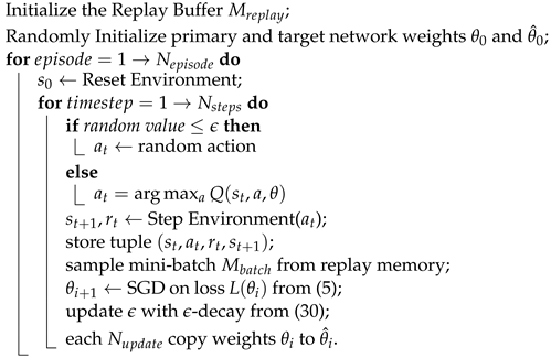
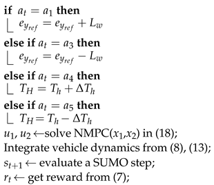
The training of the DDQN agent is summarized in Algorithms 1 and 2 as pseudo-code. At each simulation step, an action is chosen and translated into references for the NMPCs. The input signals resulting from the optimization problem solutions are then fed to the vehicle dynamics to obtain a new vehicle position to be evaluated in the highway network. The new state observations and the reward are obtained from SUMO. This procedure is repeated iteratively at each time step. The DRL agent has been trained for $N_{episode}$ = 60,000 and each episode is terminated after $N_{steps}=500$, or earlier if a collision occurs. At each sample time, the exploration constant $ϵ$ is decreased as an exponential function as:

$${ϵ}_{t+1}=(1-{ϵ}_{decay}){ϵ}_t$$

(30)

where ${ϵ}_{decay}=2.3026\times {10}^{-6}$ is the decay rate. Note thats set as the minimum exploration value is set as ${ϵ}_{end}=0.1$. The DRL agent hyper-parameters, chosen according to the state-of-art [53], are reported along with all the training parameters in

Table 3. Training and DDQN Agent Parameters.

Parameter	Value
Number of training episodes, $N_{episode}$	60,000
Number of steps per episode, $N_{steps}$	500
Sampling Time, $T_s$	0.2
Replay Memory size, $M_{replay}$	500,000
Mini-batch size, $M_{batch}$	32
Discount factor, $\gamma$	0.99
Learning rate, $\eta$	0.0005
Initial exploration constant, ${ϵ}_{start}$	1
Final exploration constant, ${ϵ}_{end}$	0.1
Exploration decay, ${ϵ}_{decay}$	2.3026 $\times {10}^{-6}$
Target Network update frequency, $N_{update}$	20,000
Input neurons, $n_{input}$	19
Number of dense layers, $n_{dense}$	2
Number of neurons for dense layers, $n_{neurons}$	128
Output neurons, $n_{output}$	5

.

Regarding the optimization procedures, due to its ability to generate highly efficient Sequence Quadratic Programming (SQP) code, we chose FORCES Pro [54] as a solver. Moreover, it can be exploited in real-time applications and presents a user-friendly MATLAB interface. Equations (8) and (13) are discretized and integrated with an explicit fourth-order Runge-Kutta algorithm. The sampling time is set as $T_s=$ 0.2 s, and both the control horizon and prediction horizon are set to $T_c=T=$ 4.0 s, for a total of twenty integration and control steps.

Algorithm1: DDQN main training loop algorithm.

Algorithm2: StepEnvironment($a_t$).

Training Results

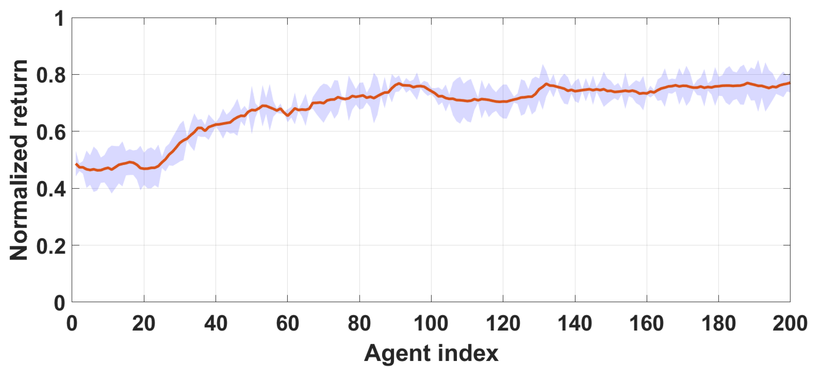
In this study, we report the results of the training phase for the DDQN agent and the overall decision-making layer. During the training phase, the agent parameters are saved and stored every 300 episodes, while in the testing phase, each saved agent’s performance is evaluated on 100 episodes of 500 maximum steps by setting the exploration factor $ϵ$ to zero. The total normalized return per episode is collected, and the mean and the variance are used as performance indexes. Figure 3 shows the result in terms of mean (red line) and variance (shaded area) for each saved agent. It can be observed how, as the training phase proceeds, the overall performance of the DRL agent increases. Despite that, due to the high variability of the road scenarios, high variance can be observed in the resulting normalized return. Moreover, even though the first agent achieves a non-zero total reward because it does not perform any lane changes, the NMPC is still capable of keeping its lane and avoiding frontal collisions. According to the reward definition in (7), we point out that a maximum reward is achieved only if the speed $v\left(t\right)$ is kept at the constant desired value $v_{des}$, without ever changing from the starting lane. Note that, these goals can be achieved only if the starting lane is always empty, and since this scenario is devoid of interest, it is therefore excluded from the training and testing phase. The last agent exhibits better performance, achieving a collision rate of around 4.0%.

Finally, we highlight that the training process is performed via an Intel^® Core${}^{\mathrm{TM}}$ i7-11900K 3.2 GHz processor, 64 GB 4.400 MHz DDR5 of RAM, GPU NVIDIA^® GeForce RTX${}^{\mathrm{TM}}$ 3080, and a Windows 11 system. The time required for the training phase, with regards to the hyper-parameters in Table 3, is approximately 20 h. It is worth noting that the training phase represents the highest computational burden required by the decision-making layer, which is, however, offline executed. Conversely, the one required to make the driving decision is very low during the deployment phase, since only the forward propagation in deep NN is involved [55].

5. Virtual Testing Simulation

Leveraging the above-mentioned co-simulation platform, the proposed control decision-making and motion planning control architectures are evaluated in non-trivial highway scenarios. For illustrative purposes, we first consider the single-lane changing scenario shown in Figure 4, where the Ego vehicle has to follow the leading one until $t=$ 100 s, when a lane-changing maneuver to the left free lane is required; afterward, the reference speed is set as $v_{ref}=$ 33 m/s. When modeling the leading vehicle in SUMO, in order to better grasp the dynamics of manually driven vehicles, we also consider the parameter called driver imperfection, which is modeled as additive noise on the acceleration command. In addition, to better show the advantages of the proposed solution, we also compare its performance with respect to the one obtained by one of the most popular state-of-the-art solutions. Specifically, the comparison analysis only involves the motion planning layer and not the decision-making one, since the performance achievable via deep learning methods is strictly correlated to the platform adopted for its design [56]. Accordingly, for the sake of fairness, we compare the NMPC with regards to the IDM solution (widely used as a benchmark for testing new control strategies [23]), both running based on the results provided by the DQN-based decision-making layer.

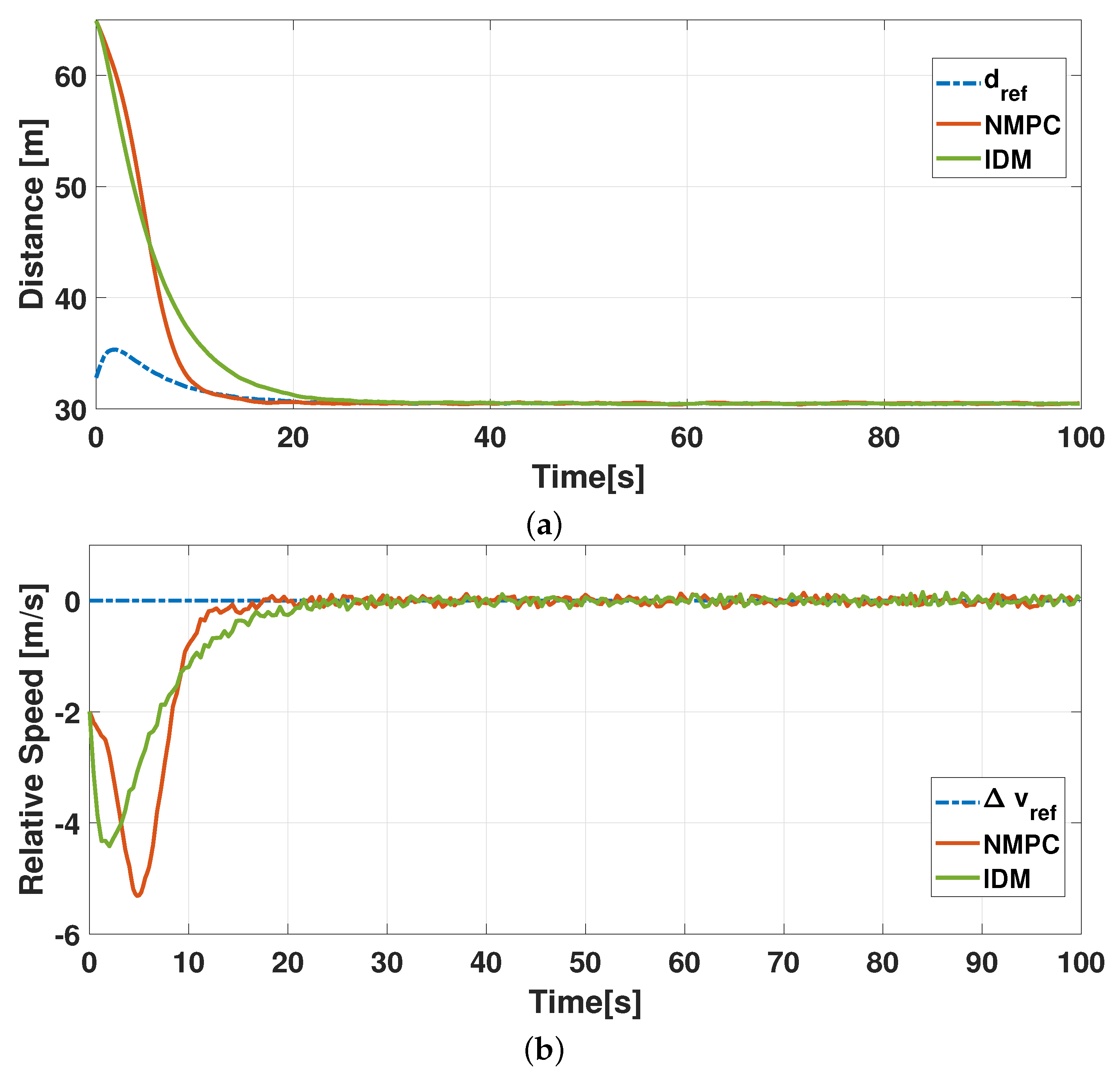
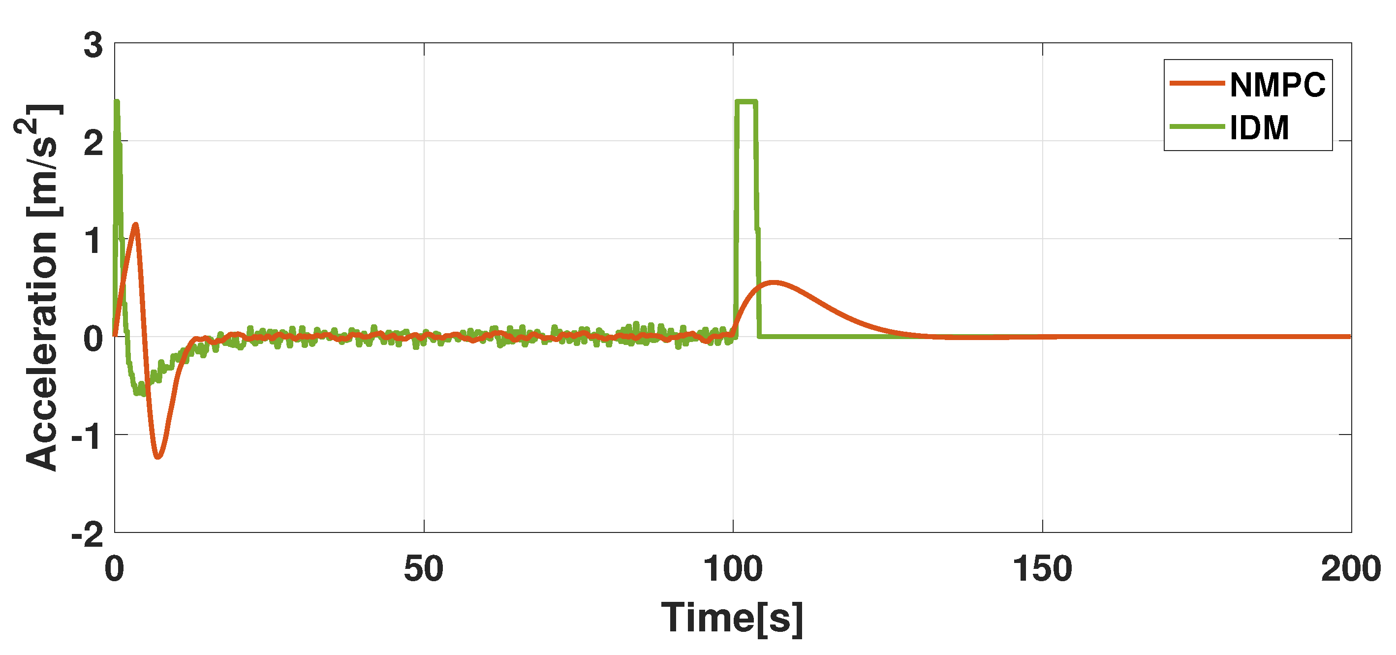
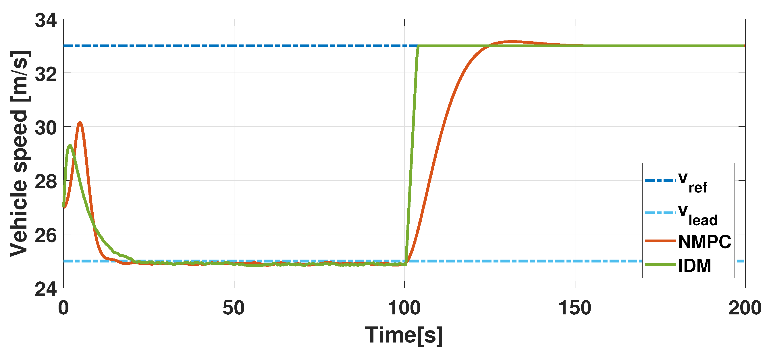
Simulation results, related to Ego vehicle longitudinal dynamics until the time instant $t=$ 100 s, are disclosed in Figure 5, where the relative distance and the relative speed of the Ego vehicle w.r.t. the leading one are depicted. Herein it can be observed how the ego vehicle reaches and maintains the desired spacing policy with regards to the preceding vehicle $d_{ref}=$ 30.6 m (see Figure 5a), while the relative speed converges towards zero (see Figure 5b). Comparison results with regards to IDM disclose the improved performances achieved by the NMPC controllers since, despite the faster convergence exhibited by these optimal techniques, the time history of the acceleration shows lower peaks, thus providing the highest driving comfort experience. This is also confirmed by Figure 6, where the acceleration trends for both NMPC and IDM are reported over the overall simulation time, i.e., $t\in [0,200]$ s. From this figure, it is possible to appreciate that, when leveraging the NMPC, lower values of the acceleration peak can be obtained. It results in a more comfortable driving experience. In fact, while the IDM reaches the saturation value of $a_{max}=$ 2.4 m/s${}^2$, the resulting acceleration computed by the NMPC case is always below the value of $a=$ 1.2 m/s${}^2$. Moreover, it is worthy to point out that the presence of noise, arising from the implementation of driver model for the leading vehicle in SUMO, clearly affects the IDM performances, while NMPC shows enhanced resilience. The vehicle speed $v\left(t\right)$ and lateral position $e_y\left(t\right)$ profiles are, instead, depicted in Figure 7 and Figure 8, respectively. Specifically, simulation results in Figure 7 confirm that the ego vehicle keeps the leading speed, namely $v_{lead}=$ 25 m/s, until the time instant of 100 s when the lane-change maneuver to the left is performed; then, its speed reaches the desired reference value of $v_{ref}=$ 33 m/s. Once more, the NMPC is able to provide a more comfortable driving experience with respect to the IDM since the desired set-point is reached with smoother behavior (see also Figure 6). Moreover, during the lane changing maneuver, the Ego vehicle’s lateral position $e_y\left(t\right)$ is equal to zero before the time instant $t=100$ s and, afterwards, it is correctly regulated to $e_{y_{ref}}=L_w=$ 3.6 m (the left lane center-line) (see Figure 8).

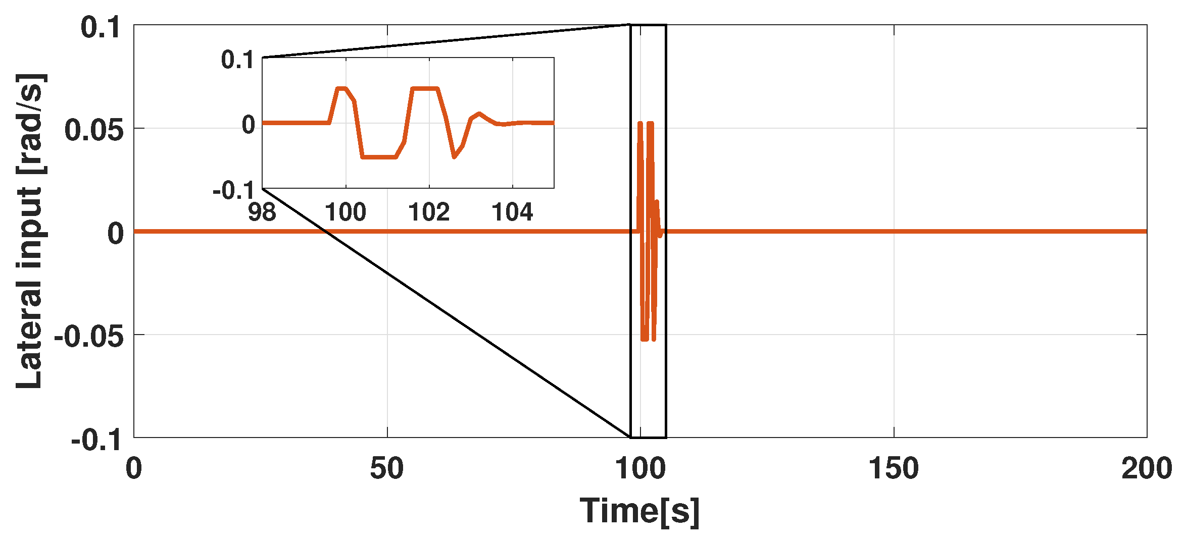
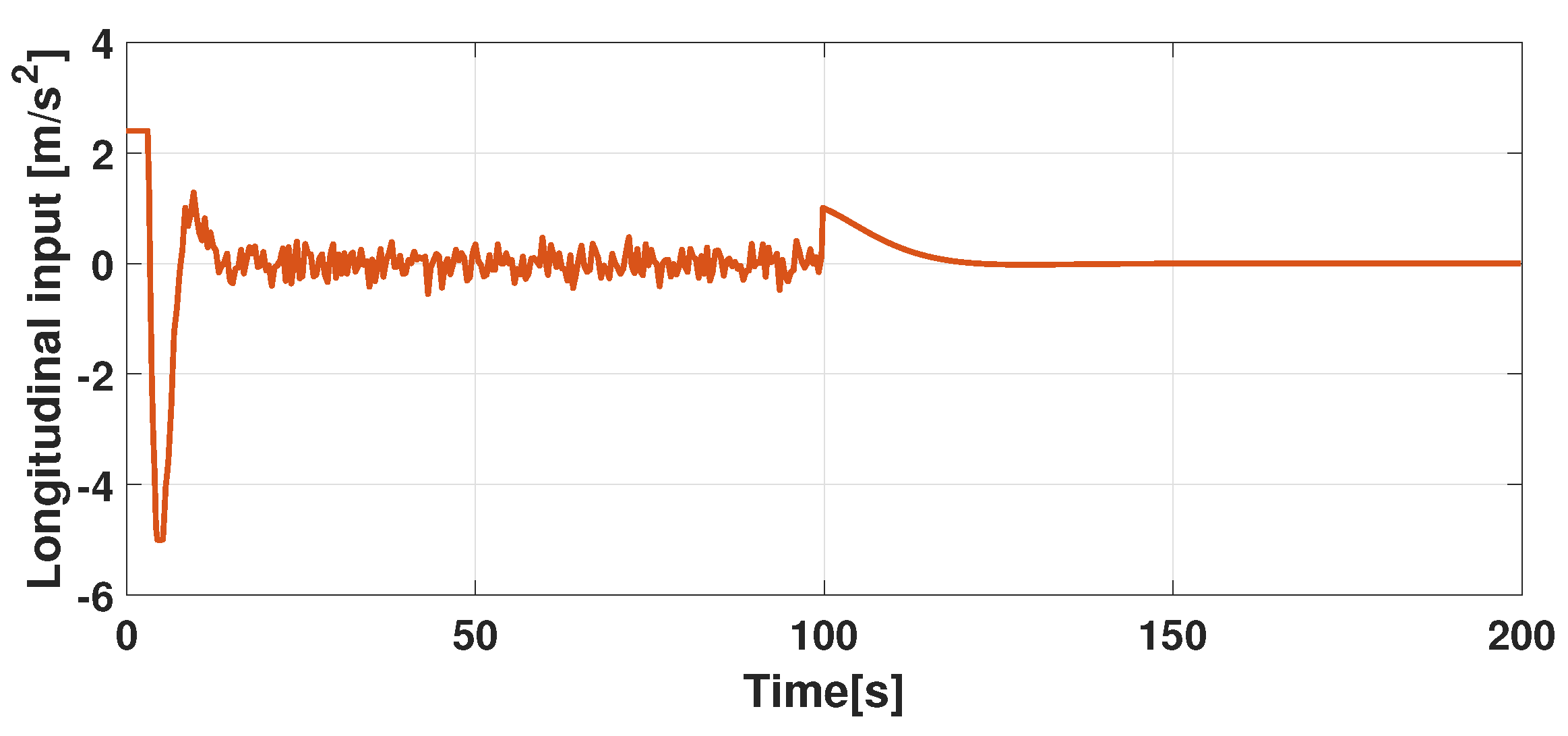
In order to provide more insights on the behaviour and performance achieved by the NMPC, Figure 9 and Figure 10 show the time history of the lateral and longitudinal control inputs, $u_1\left(t\right)$ and $u_2\left(t\right)$, respectively. Results show that, as expected, the dynamics of these input variables are always smooth and well-bounded, thus backing up the comfort results shown in the previous figures, and that the NMPC enables us to tune the right trade-off between aggressiveness and comfort in a straightforward manner; this also ensures that the input constraints are never violated. Finally, to evaluate the real-time performance of the proposed hybrid control architecture, we evaluate its computational load via the Simulink Profiler Tool [2]. By leveraging the same hardware used in the training phase, the simulation profile reports that the required total computational times are 3.75 s and 19.05 s for the DQN agent and NMPC controller, respectively, w.r.t. an overall simulation time of 200 s.

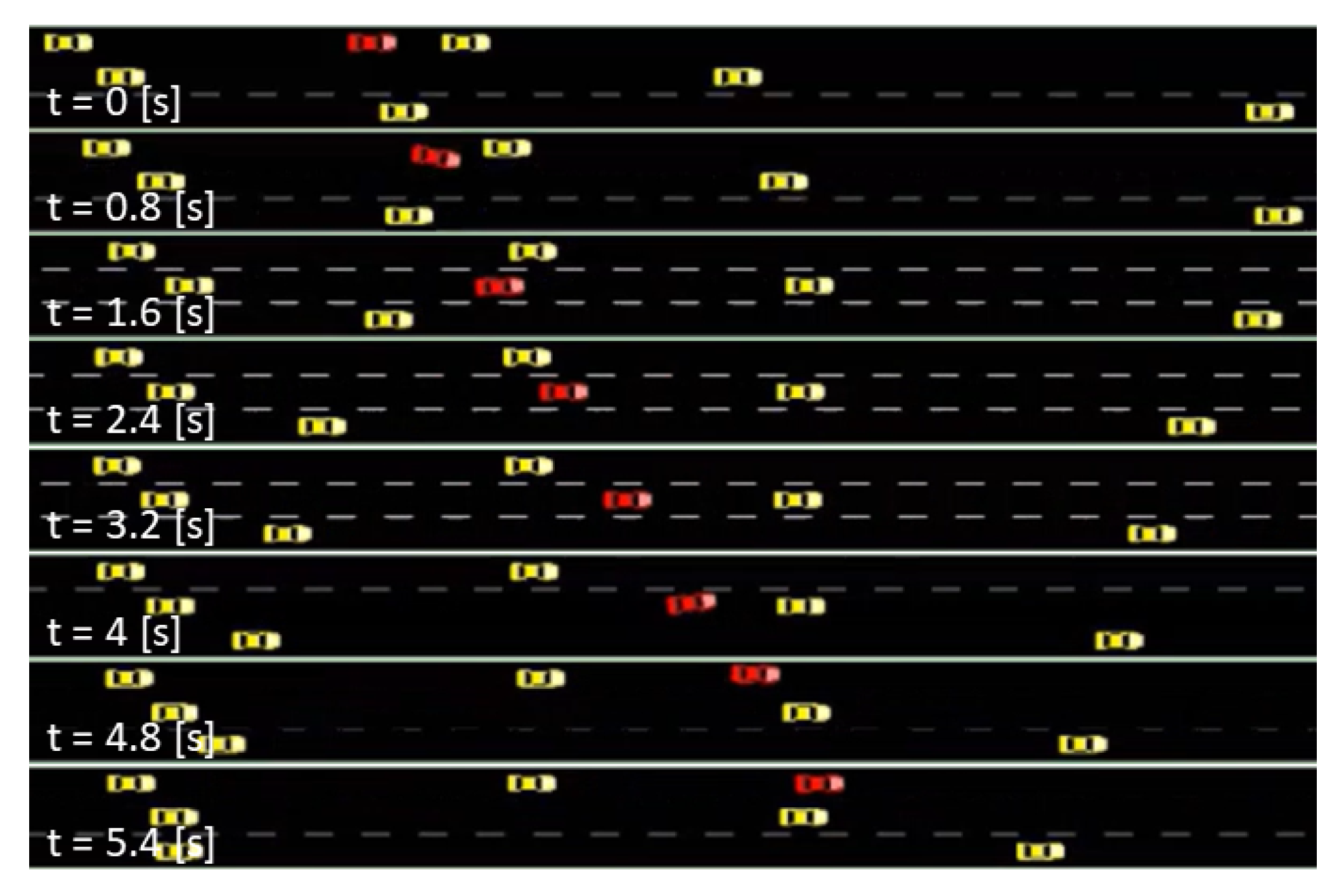
As a more exhaustive validation scenario, we consider a three-lane highway scenario characterized by heavy traffic conditions, i.e., a lane count of 1500 vehicles per hour. The vehicles along the lanes travel at different random constant speeds. However, under heavy-density traffic conditions, they vary their velocities according to the traffic flow and perform lane-changing maneuvres both on the right and on the left lane, when necessary. In this highly uncertain scenario, the proposed hybrid control architecture drives the Ego vehicle in performing safe lane-changing maneuvers to the right and left according to the encountered traffic scenario. An exemplary visualization of this appraised scenario is shown in Figure 11, where the ego vehicle performs a lane change maneuver to the right in order to gain speed. Detailed results about this complex scenario, reported at https://youtu.be/Srj7TXdrKhY (accessed on 6 March 2023), confirm the ability of the proposed hybrid architecture in safely driving the Ego vehicle under highly-varying traffic conditions, as well as its effectiveness in facing the uncertainties arising from unexpected and sudden lane changing maneuvers performed by the surrounding vehicles.

6. Conclusions

In this paper, a novel hybrid hierarchical decision-making and motion planning control architecture for Autonomous Vehicles, driving in uncertain and unknown highway environments has been addressed. The high-level decision-making, designed via the emerging Deep Reinforcement Learning theory, has allowed the AV to learn how to adapt, in real-time, its driving behavior according to the current surrounding highway environment and, hence, how to take the proper longitudinal and lateral autonomous decisions to avoid collisions and improve travel safety. The decision-making process has been carried out by exploiting a proper reward function that penalizes hazardous and non-safe maneuvers. The training of the DDQN agent has been performed by leveraging a high-fidelity co-simulation platform, and the results have confirmed the correct learning process in this highly uncertain driving scenario, whose features are difficult to capture via classical model-based approaches. These optimal driving policies represent the reference behavior for the motion planning layer, where optimal controllers based on NMPC have been responsible for the optimized driving behaviors, also enforcing constraints in the state/control of the ego vehicle. The validation of the designed architecture, carried out by also considering an high-density traffic flow, has disclosed how the vehicle, thanks to the high decision-level was able to select, according to the current highway driving situations, the proper safe maneuver (i.e., lane changing, overtaking of acceleration/braking maneuvers) to engage, while the low-level determines the optimal control commands to be imposed on the AV (explicitly considering its dynamic constraints) for ensuring a safe tracking of the selected driving mode. Summarizing, the virtual simulations in non-trivial highway traffic scenarios have confirmed the effectiveness of the proposed hybrid architecture and its advantages in combining model-based and artificial intelligence-based methods. Future work will involve the extension of the approach to different road geometries and urban environments.

References

1. Rojas-Rueda, D.; Nieuwenhuijsen, M.J.; Khreis, H.; Frumkin, H. Autonomous vehicles and public health. Annu. Rev. Public Health 2020, 41, 329–345. [Google Scholar] [CrossRef] [PubMed]
2. Caiazzo, B.; Coppola, A.; Petrillo, A.; Santini, S. Distributed nonlinear model predictive control for connected autonomous electric vehicles platoon with distance-dependent air drag formulation. Energies 2021, 14, 5122. [Google Scholar] [CrossRef]
3. Caiazzo, B.; Lui, D.G.; Petrillo, A.; Santini, S. Distributed Double-Layer Control for Coordination of Multi-Platoons approaching road restriction in the presence of IoV communication delays. IEEE Internet Things J. 2021, 9, 4090–4109. [Google Scholar] [CrossRef]
4. Coppola, A.; Lui, D.G.; Petrillo, A.; Santini, S. Eco-Driving Control Architecture for Platoons of Uncertain Heterogeneous Nonlinear Connected Autonomous Electric Vehicles. IEEE Trans. Intell. Transp. Syst. 2022, 23, 24220–24234. [Google Scholar] [CrossRef]
5. Coppola, A.; Lui, D.G.; Petrillo, A.; Santini, S. Cooperative Driving of Heterogeneous Uncertain Nonlinear Connected and Autonomous Vehicles via Distributed Switching Robust PID-like Control. Inf. Sci. 2023, 625, 277–298. [Google Scholar] [CrossRef]
6. Liu, W.; Hua, M.; Deng, Z.; Huang, Y.; Hu, C.; Song, S.; Gao, L.; Liu, C.; Xiong, L.; Xia, X. A Systematic Survey of Control Techniques and Applications: From Autonomous Vehicles to Connected and Automated Vehicles. arXiv 2023, arXiv:2303.05665. [Google Scholar]
7. Zong, W.; Zhang, C.; Wang, Z.; Zhu, J.; Chen, Q. Architecture design and implementation of an autonomous vehicle. IEEE Access 2018, 6, 21956–21970. [Google Scholar] [CrossRef]
8. Peng, J.; Zhang, S.; Zhou, Y.; Li, Z. An Integrated Model for Autonomous Speed and Lane Change Decision-Making Based on Deep Reinforcement Learning. IEEE Trans. Intell. Transp. Syst. 2022, 23, 21848–21860. [Google Scholar] [CrossRef]
9. Urmson, C.; Anhalt, J.; Bagnell, D.; Baker, C.; Bittner, R.; Clark, M.; Dolan, J.; Duggins, D.; Galatali, T.; Geyer, C.; et al. Autonomous driving in urban environments: Boss and the urban challenge. J. Field Robot. 2008, 25, 425–466. [Google Scholar] [CrossRef]
10. Kyprianou, G.; Doitsidis, L.; Chatzichristofis, S. Towards the Achievement of Path Planning with Multi-robot Systems in Dynamic Environments. J. Intell. Robot. Syst. 2022, 104, 1–18. [Google Scholar]
11. Di Vaio, M.; Fiengo, G.; Petrillo, A.; Salvi, A.; Santini, S.; Tufo, M. Cooperative shock waves mitigation in mixed traffic flow environment. IEEE Trans. Intell. Transp. Syst. 2019, 20, 4339–4353. [Google Scholar] [CrossRef]
12. Zhang, S.; Wu, Y.; Ogai, H.; Inujima, H.; Tateno, S. Tactical decision-making for autonomous driving using dueling double deep Q network with double attention. IEEE Access 2021, 9, 151983–151992. [Google Scholar] [CrossRef]
13. Baierle, I.C.; Sellitto, M.A.; Frozza, R.; Schaefer, J.L.; Habekost, A.F. An artificial intelligence and knowledge-based system to support the decision-making process in sales. S. Afr. J. Ind. Eng. 2019, 30, 17–25. [Google Scholar] [CrossRef]
14. Sardjono, W.; Lusia, E.; Utomo, H.; Sukardi, S.; Rahmasari, A.; Regent Montororing, Y.D. Competitive Advantage Model Through Knowledge Management Systems Implementation to Optimize Business Sustainability. In Proceedings of the 2021 The 9th International Conference on Information Technology: IoT and Smart City, Guangzhou, China, 22–25 November 2021; pp. 154–160. [Google Scholar]
15. Yu, J.B.; Yu, Y.; Wang, L.N.; Yuan, Z.; Ji, X. The knowledge modeling system of ready-mixed concrete enterprise and artificial intelligence with ANN-GA for manufacturing production. J. Intell. Manuf. 2016, 27, 905–914. [Google Scholar] [CrossRef]
16. Li, G.; Yang, Y.; Li, S.; Qu, X.; Lyu, N.; Li, S.E. Decision making of autonomous vehicles in lane change scenarios: Deep reinforcement learning approaches with risk awareness. Transp. Res. Part Emerg. Technol. 2021, 134, 103452. [Google Scholar] [CrossRef]
17. Lu, Y.; Xu, X.; Zhang, X.; Qian, L.; Zhou, X. Hierarchical reinforcement learning for autonomous decision making and motion planning of intelligent vehicles. IEEE Access 2020, 8, 209776–209789. [Google Scholar] [CrossRef]
18. Liao, J.; Liu, T.; Tang, X.; Mu, X.; Huang, B.; Cao, D. Decision-Making Strategy on Highway for Autonomous Vehicles Using Deep Reinforcement Learning. IEEE Access 2020, 8, 177804–177814. [Google Scholar] [CrossRef]
19. Nageshrao, S.; Tseng, H.E.; Filev, D. Autonomous highway driving using deep reinforcement learning. In Proceedings of the 2019 IEEE International Conference on Systems, Man and Cybernetics (SMC), Bari, Italy, 6–9 October 2019; pp. 2326–2331. [Google Scholar]
20. Baheri, A.; Nageshrao, S.; Tseng, H.E.; Kolmanovsky, I.; Girard, A.; Filev, D. Deep reinforcement learning with enhanced safety for autonomous highway driving. In Proceedings of the 2020 IEEE Intelligent Vehicles Symposium (IV), Anchorage, Alaska, USA, 4–7 June 2023; pp. 1550–1555. [Google Scholar]
21. Bifulco, G.N.; Coppola, A.; Petrillo, A.; Santini, S. Decentralized cooperative crossing at unsignalized intersections via vehicle-to-vehicle communication in mixed traffic flows. J. Intell. Transp. Syst. 2022. [Google Scholar] [CrossRef]
22. Albeaik, S.; Bayen, A.; Chiri, M.T.; Gong, X.; Hayat, A.; Kardous, N.; Keimer, A.; McQuade, S.T.; Piccoli, B.; You, Y. Limitations and improvements of the intelligent driver model (IDM). SIAM J. Appl. Dyn. Syst. 2022, 21, 1862–1892. [Google Scholar] [CrossRef]
23. Albaba, B.M.; Yildiz, Y. Driver modeling through deep reinforcement learning and behavioral game theory. IEEE Trans. Control Syst. Technol. 2021, 30, 885–892. [Google Scholar] [CrossRef]
24. Erke, S.; Bin, D.; Yiming, N.; Qi, Z.; Liang, X.; Dawei, Z. An improved A-Star based path planning algorithm for autonomous land vehicles. Int. J. Adv. Robot. Syst. 2020, 17, 1729881420962263. [Google Scholar] [CrossRef]
25. Szczepanski, R.; Tarczewski, T.; Erwinski, K. Energy efficient local path planning algorithm based on predictive artificial potential field. IEEE Access 2022, 10, 39729–39742. [Google Scholar] [CrossRef]
26. Spanogiannopoulos, S.; Zweiri, Y.; Seneviratne, L. Sampling-based non-holonomic path generation for self-driving cars. J. Intell. Robot. Syst. 2022, 104, 1–17. [Google Scholar]
27. Lee, K.; Kum, D. Collision avoidance/mitigation system: Motion planning of autonomous vehicle via predictive occupancy map. IEEE Access 2019, 7, 52846–52857. [Google Scholar] [CrossRef]
28. Wang, H.; Huang, Y.; Khajepour, A.; Zhang, Y.; Rasekhipour, Y.; Cao, D. Crash mitigation in motion planning for autonomous vehicles. IEEE Trans. Intell. Transp. Syst. 2019, 20, 3313–3323. [Google Scholar] [CrossRef]
29. Li, G.; Yang, Y.; Zhang, T.; Qu, X.; Cao, D.; Cheng, B.; Li, K. Risk assessment based collision avoidance decision-making for autonomous vehicles in multi-scenarios. Transp. Res. Part Emerg. Technol. 2021, 122, 102820. [Google Scholar] [CrossRef]
30. Xu, X.; Zuo, L.; Li, X.; Qian, L.; Ren, J.; Sun, Z. A reinforcement learning approach to autonomous decision making of intelligent vehicles on highways. IEEE Trans. Syst. Man, Cybern. Syst. 2018, 50, 3884–3897. [Google Scholar] [CrossRef]
31. Celemin, C.; Ruiz-del Solar, J. An interactive framework for learning continuous actions policies based on corrective feedback. J. Intell. Robot. Syst. 2019, 95, 77–97. [Google Scholar] [CrossRef]
32. Matsuo, Y.; LeCun, Y.; Sahani, M.; Precup, D.; Silver, D.; Sugiyama, M.; Uchibe, E.; Morimoto, J. Deep learning, reinforcement learning, and world models. Neural Netw. 2022, 152, 267–275. [Google Scholar] [CrossRef]
33. Candeli, A.; De Tommasi, G.; Lui, D.G.; Mele, A.; Santini, S.; Tartaglione, G. A Deep Deterministic Policy Gradient Learning Approach to Missile Autopilot Design. IEEE Access 2022, 10, 19685–19696. [Google Scholar] [CrossRef]
34. Basile, G.; Lui, D.G.; Petrillo, A.; Santini, S. Deep Deterministic Policy Gradient-based Virtual Coupling Control For High-Speed Train Convoys. In Proceedings of the 2022 IEEE International Conference on Networking, Sensing and Control (ICNSC), Shanghai, China, 15–18 December 2022; pp. 1–6. [Google Scholar]
35. Gu, S.; Lillicrap, T.; Sutskever, I.; Levine, S. Continuous deep q-learning with model-based acceleration. In Proceedings of the International Conference on Machine Learning, New York, NY, USA, 19–24 June 2016; pp. 2829–2838. [Google Scholar]
36. Rodriguez-Ramos, A.; Sampedro, C.; Bavle, H.; De La Puente, P.; Campoy, P. A deep reinforcement learning strategy for UAV autonomous landing on a moving platform. J. Intell. Robot. Syst. 2019, 93, 351–366. [Google Scholar] [CrossRef]
37. Wang, P.; Chan, C.Y.; de La Fortelle, A. A reinforcement learning based approach for automated lane change maneuvers. In Proceedings of the 2018 IEEE Intelligent Vehicles Symposium (IV), Suzhou, China, 26–30 June 2018; pp. 1379–1384. [Google Scholar]
38. Moghadam, M.; Elkaim, G.H. A hierarchical architecture for sequential decision-making in autonomous driving using deep reinforcement learning. arXiv 2019, arXiv:1906.08464. [Google Scholar]
39. Lubars, J.; Gupta, H.; Chinchali, S.; Li, L.; Raja, A.; Srikant, R.; Wu, X. Combining reinforcement learning with model predictive control for on-ramp merging. In Proceedings of the 2021 IEEE International Intelligent Transportation Systems Conference (ITSC), Indianapolis, IN, USA, 19–22 September 2021; pp. 942–947. [Google Scholar]
40. Zanon, M.; Gros, S. Safe reinforcement learning using robust MPC. IEEE Trans. Autom. Control 2020, 66, 3638–3652. [Google Scholar] [CrossRef]
41. Zheng, Y.; Ding, W.; Ran, B.; Qu, X.; Zhang, Y. Coordinated decisions of discretionary lane change between connected and automated vehicles on freeways: A game theory-based lane change strategy. IET Intell. Transp. Syst. 2020, 14, 1864–1870. [Google Scholar] [CrossRef]
42. Yavas, U.; Kumbasar, T.; Ure, N.K. A new approach for tactical decision making in lane changing: Sample efficient deep Q learning with a safety feedback reward. In Proceedings of the 2020 IEEE Intelligent Vehicles Symposium (IV), Las Vegas, NV, USA, 19 October–13 November 2020; pp. 1156–1161. [Google Scholar]
43. Sheng, Z.; Liu, L.; Xue, S.; Zhao, D.; Jiang, M.; Li, D. A Cooperation-Aware Lane Change Method for Autonomous Vehicles. arXiv 2022, arXiv:2201.10746. [Google Scholar]
44. Watkins, C.J.; Dayan, P. Q-learning. Mach. Learn. 1992, 8, 279–292. [Google Scholar] [CrossRef]
45. Rajamani, R. Vehicle Dynamics and Control; Springer Science & Business Media: Berlin/Heidelberg, Germany, 2011. [Google Scholar]
46. Polack, P.; Altché, F.; Novel, B.; de La Fortelle, A. The kinematic bicycle model: A consistent model for planning feasible trajectories for autonomous vehicles? In Proceedings of the 2017 IEEE Intelligent Vehicles Symposium (IV), Los Angeles, CA, USA, 11–14 June 2017; pp. 812–818. [Google Scholar] [CrossRef]
47. Liu, W.; Xia, X.; Xiong, L.; Lu, Y.; Gao, L.; Yu, Z. Automated vehicle sideslip angle estimation considering signal measurement characteristic. IEEE Sens. J. 2021, 21, 21675–21687. [Google Scholar] [CrossRef]
48. Xia, X.; Hashemi, E.; Xiong, L.; Khajepour, A. Autonomous Vehicle Kinematics and Dynamics Synthesis for Sideslip Angle Estimation Based on Consensus Kalman Filter. IEEE Trans. Control Syst. Technol. 2022, 31, 179–192. [Google Scholar] [CrossRef]
49. Xiong, L.; Xia, X.; Lu, Y.; Liu, W.; Gao, L.; Song, S.; Yu, Z. IMU-based automated vehicle body sideslip angle and attitude estimation aided by GNSS using parallel adaptive Kalman filters. IEEE Trans. Veh. Technol. 2020, 69, 10668–10680. [Google Scholar] [CrossRef]
50. Liu, W.; Xiong, L.; Xia, X.; Lu, Y.; Gao, L.; Song, S. Vision-aided intelligent vehicle sideslip angle estimation based on a dynamic model. IET Intell. Transp. Syst. 2020, 14, 1183–1189. [Google Scholar] [CrossRef]
51. Borrelli, F.; Falcone, P.; Keviczky, T.; Asgari, J.; Hrovat, D. MPC-based approach to active steering for autonomous vehicle systems. Int. J. Veh. Auton. Syst. 2005, 3, 265–291. [Google Scholar] [CrossRef]
52. Teng, S.; Deng, P.; Li, Y.; Li, B.; Hu, X.; Xuanyuan, Z.; Chen, L.; Ai, Y.; Li, L.; Wang, F.Y. Path Planning for Autonomous Driving: The State of the Art and Perspectives. arXiv 2023, arXiv:2303.09824. [Google Scholar]
53. Hoel, C.J.; Wolff, K.; Laine, L. Automated speed and lane change decision making using deep reinforcement learning. In Proceedings of the 2018 21st International Conference on Intelligent Transportation Systems (ITSC), Maui, HI, USA, 4–7 November 2018; pp. 2148–2155. [Google Scholar]
54. Domahidi, A.; Jerez, J.; FORCES Professional. Embotech AG, 2014–2019. Available online: https://embotech.com/FORCES-Pro (accessed on 6 March 2023).
55. Lei, L.; Liu, T.; Zheng, K.; Hanzo, L. Deep reinforcement learning aided platoon control relying on V2X information. IEEE Trans. Veh. Technol. 2022, 71, 5811–5826. [Google Scholar] [CrossRef]
56. Gao, C.; Yan, J.; Zhou, S.; Varshney, P.K.; Liu, H. Long short-term memory-based deep recurrent neural networks for target tracking. Inf. Sci. 2019, 502, 279–296. [Google Scholar] [CrossRef]
Figure 1. Autonomous Highway Driving problem. The Ego vehicle, i.e., the red one, has to autonomously take a safe driving decision, e.g., lane keeping or changing, for traveling in a three-lane highway scenario in the presence of other surrounding vehicles, i.e., the grey ones.
Energies 16 03490 g001
Figure 2. Hybrid Hierarchical decision-making and motion planning control architecture. The proposed solution driving the motion of the Ego-vehicles runs on the MATLAB Platform, while the interactions between the ego vehicle and the other road entities are emulated by exploiting SUMO.
Energies 16 03490 g002
Figure 3. Training results of the DQN agent. Trend of the normalized reward over the evaluated agent index. The red line is the mean while the shaded blue area is the variance over 100 episodes per agents.
Energies 16 03490 g003
Figure 4. Visualization of the single lane changing scenario around t = 100 s.
Energies 16 03490 g004
Figure 5. Single lane changing scenario. Performance of the proposed solution until the time instant t = 100 [ s ] and comparison analysis w.r.t. IDM solution. Time-history of: (a) relative distance d ( t ) between the Ego vehicle and the leading one; (b) relative speed Δ v ( t ) between the ego and leading vehicles.
Energies 16 03490 g005
Figure 6. Single lane changing scenario. Performance of the proposed solution and comparison analysis w.r.t. IDM solution. Time-history of the ego vehicle acceleration a ( t ) .
Energies 16 03490 g006
Figure 7. Single lane changing scenario. Performance of the proposed solution and comparison analysis w.r.t. IDM solution. Time-history of the longitudinal Ego vehicle speed v ( t ) .
Energies 16 03490 g007
Figure 8. Single lane changing scenario. Performance of the proposed solution and comparison analysis w.r.t. IDM solution. Time-history of the Ego vehicle lateral position e y ( t ) .
Energies 16 03490 g008
Figure 9. Single lane changing scenario. Performance of the proposed solution and comparison analysis w.r.t. IDM solution. Time-history of the ego vehicle lateral input u 1 ( t ) .
Energies 16 03490 g009
Figure 10. Single lane change scenario. Performance of the proposed solution. Time-history of the ego vehicle longitudinal input u 2 ( t ) .
Energies 16 03490 g010
Figure 11. Sequence of extracted frames from an exemplary scenario. The ego vehicle (in red) changes lane to the right so to overtake the front vehicle and gain speed. The time initiation is appropriate to avoid a collision with rear vehicles.
Energies 16 03490 g011