Abstract
The in-vessel Loss-of-Coolant Accident (LOCA) is one of the design basis accidents in the design of the EU DEMO tokamak fusion reactor. System-level codes are typically employed to analyse the evolution of these transients. However, being based on a lumped approach, they are unable to quantify localised quantities of interest, such as local pressure peaks on the vacuum vessel walls, to which the failure criteria are linked. To calculate local quantities, the 3D nature of the phenomenon needs to be considered. In this work, a 3D transient model of the in-vessel LOCA from a water-cooled blanket is developed. The model is implemented in the commercial CFD software STAR-CCM+. It simulates the propagation of the water jet in the vessel from the beginning of the accident, thus accounting for the phase change of the water, i.e., from the pressurised liquid phase to the vapour phase inside the vessel, being the latter at a much lower pressure than in the blanket coolant pipes. Due to the large pressure ratio (>1000), shocks are expected; therefore, an Adaptive Mesh Refinement (AMR) algorithm is employed. The physical models (in particular, the multiphase model) are benchmarked to a 2D reference problem before being applied to the 3D EU DEMO-relevant problem. The simulation results show that the pressure peaks in front of the vessel walls are not dangerous as they are below the design limit. The entire evolution of the water jet is followed up to the opening of the burst disks, in order to compare the average pressure evolution with that computed with system-level codes. A comparison with the in-vessel LOCA from a helium-cooled blanket is also carried out, showing that the accident evolution in the water case is less violent than in the helium case.
1. Introduction
The design of safety systems is a key part of the conceptual design phase of the EU DEMO tokamak fusion reactor [1,2,3], including the Vacuum Vessel Pressure Suppression System (VVPSS) [4,5], which will be responsible for the mitigation of accidents such as an in-vessel Loss-of-Coolant Accident (LOCA). One of the possible initiating events of this type of accident is a break in the First Wall (FW), cooled by a high-pressure coolant, which, when released inside the vacuum vessel (VV), would increase its pressure above the operating limit of 2 bar [6].
A system-level, 0D/1D approach is usually employed for this type of analysis, following experience from fission power plants, adopting tools such as, e.g., RELAP [7,8], MELCOR [9,10], CONSEN [11,12], or GETTHEM [13,14]; however, as opposed to fission reactors, where the failure criterion can be identified as global parameters (e.g., core uncovery), for the VV failure, the criterion is local, being linked to the pressure on a specific surface (i.e., the gyrotron diamond windows). Therefore, the validity of a global approach is questionable and needs to be checked carefully [15]. This check can be carried out only by means of 3D analyses with detailed tools such as Computational Fluid Dynamics (CFD).
In this work, a 3D CFD transient model is developed, to simulate the evolution of the transient when the released coolant is pressurised water; the model has similar features with respect to that presented in [15] for the case of a helium coolant, with, however, some important differences due to the two-phase flow, developed when the high-pressure water is released in the low-pressure environment of the VV.
The paper is organised as follows: in Section 2, the assumed scenario and geometry are described, including the relevant simplifications introduced; in Section 3, the simulation setup is presented, including the boundary and initial conditions, adopted models and solvers, and mesh; the results are presented in Section 4 and compared, in Section 5, to the analysis carried out in [15], and the conclusions and future activities are reported in Section 6.
2. Scenario and Geometry Description
The scenario taken into account is a LOCA inside the VV of the EU DEMO fusion reactor. The accident originates after the occurrence of an unprotected plasma transient event, which causes the breakage of a portion of the FW, exposing its coolant channels and causing the release of the coolant. As water is considered as a coolant, the conditions relevant to the Water-Cooled Lithium-Lead Breeding Blanket (WCLL-BB) concept [16] are considered, which foresees the use of water in thermodynamic conditions equivalent to that of a pressurised water reactor (i.e., 155 bar, 295–328 °C).
The cooling water is then rapidly released inside the plasma chamber—see Figure 1—in the form of a two-phase flashing jet. To mitigate the accident’s consequences, the VV is equipped with one or more burst disks (BD), which separate the VV from the VVPSS. When the pressure on their surface reaches 1.5 bar, the BDs will open automatically, allowing the communication between the two environments. The analysed transient begins with the occurrence of the break (at = 0 s) and ends when the volume-averaged pressure reaches 1.5 bar.

Figure 1.
The EU DEMO tokamak [17].
Due to the complexity of the geometry, different simplifications are introduced in order to reduce the computational burden. First of all, the fluid domain is approximated as the plasma chamber, thus neglecting the flow through the gaps between the different BB segments (2 cm), since it is expected not to impact the result of the current analysis. Then, in order to further reduce the computational domain, the divertor region is not considered. This allows one to exploit both an up-down and a left-right symmetry. Nevertheless, the overall volume simulated is kept equal to a fourth of the original one (∼750 m), thus considering also the volume that would be occupied by the diverter.
The inlet section area, consistently with the scenario taken into account, involves the failure of a 1 m portion of the BB, which, according to the actual configuration of the WCLL, would cause the breakage of 262 cooling channels with the consequent discharge of water. For computational reasons, the adopted inlet flow area is evaluated as twice the sum of all 262 channel sections (to account for the double-ended rupture), for a total area of ∼0.0308 m. Since a symmetric domain is used, the inlet region is imposed equal to a circular area with the same cross-section, according to
where D is the diameter of the inlet region.
3. Simulation Setup
In this section, the setup adopted for the CFD model is described. The software used for the simulation is STAR-CCM+ v.2021.2 [18].
3.1. Boundary and Initial Conditions
3.1.1. Boundary Conditions
The boundary conditions selected are reported in Figure 2: the “stagnation inlet” is the boundary condition used by the software to impose total pressure and temperature values, as well as the void fraction (for multiphase problems), at an inlet [18].
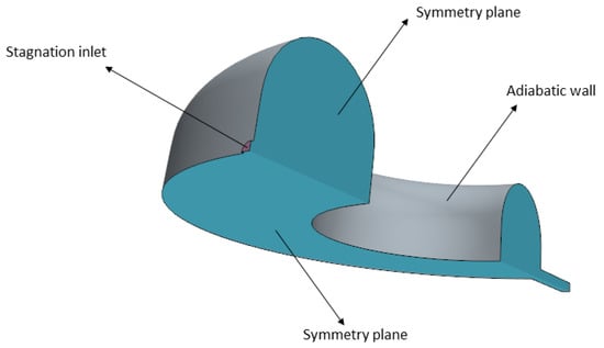
Figure 2.
Computational domain and boundary conditions [15].
This type of boundary condition requires both the static pressure and the total pressure to be specified at the inlet. In particular, the total pressure can be retrieved by the following equation:
where is the ratio of specific heats of the gas, and is the Mach number (ratio between the fluid speed at the boundary and the speed of sound in the medium); as is an output of the simulation, it is computed at each solver iteration on the inlet surface and substituted in Equation (2). Additionally, the total temperature is prescribed, according to
where is the static temperature (311.5 °C), and is computed at each iteration as discussed above.
The time span of interest in this simulation is of a few seconds, while the time needed for the Primary Heat Transfer System (PHTS) to depressurise is in the order of tens of seconds, with the exception of the very first instants when the PHTS rapidly moves from the design pressure to the saturation pressure [13,14]. However, as explained in Section 3.1.2 below, the transient immediately after the break is beyond the scope of this work as it cannot be modelled with a CFD tool; therefore, a constant inlet static pressure is assumed, and it is conservatively set equal to the design value (155 bar), giving an initial pressure ratio of 1550.
3.1.2. Initial Conditions
The vacuum chamber, for computational reasons, is considered filled with water vapour at a static pressure of 0.1 bar and with a temperature of 45.8 °C. The value of the static pressure is chosen so that the continuum assumption could be verified, i.e., in order to have a low Knudsen number (∼1 ), where is defined as follows:
with:
- : molecular mean free path;
- L: characteristic length (in this case, the distance between the inlet and the wall in front of it);
- : Boltzmann constant;
- T: temperature of the system;
- : particle diameter;
- p: pressure of the system.
As discussed in [15], this assumption could be considered equivalent to an evaluation of the transient after the initial instants, when the continuum hypothesis begins to hold.
Concerning the temperature condition, the actual value during such a phenomenon is not known. According to different 0D analyses of in-vessel LOCAs found in the literature, the initial VV temperatures may range from 290 K to 600 K (see, e.g., [9,13,19]). Nevertheless, its evolution is almost independent of the initial condition; see, e.g., [20].
3.2. Model and Solvers
3.2.1. Model
The problem under analysis requires a multiphase approach, in order to account for the phase change due to the flashing of the water from liquid to vapour. A first choice must be made among the different models available in the software to solve the equation of state and the phase interaction. In this case, the Volume of Fluid (VOF) model is selected. The suitability of this approach in modelling the phase change under analysis has been checked and benchmarked against literature results, as described in Appendix A. Furthermore, it allows the activation of a compressibility enhancement option that improves the model’s ability to solve highly compressible flows () [18]. In order to capture the flashing phenomenon close to the inlet, the Homogeneous Relaxation Model (HRM) has also been selected among the optional models available in the software to solve the phase interaction. Due to the nature of flash boiling (i.e., phase change in thermal non-equilibrium conditions), the HRM is particularly suitable for the case under examination; see [21] for a detailed comparison with other simpler models, as it is based on a finite rate equation for the rate of change of the vapour mass fraction.
Concerning the set of Navier–Stokes equations, the choice is dictated by the multiphase model selected, which, in this case, allows only the use of the segregated approach (enabled with the “segregated flow” and “segregated fluid temperature” models).
The local Reynolds number, computed according to equation
where is the fluid density, v is the average speed, and is the fluid dynamic viscosity, is >4 inside the jet region during the whole transient. This means that the flow regime is fully turbulent and, based on [18], the realisable two-layer turbulence model has been chosen for the analysis.
3.2.2. Solvers
The complexity of the problem at hand requires also the solver settings to be properly tuned. A list of the adopted solvers is reported below.
- Implicit Unsteady.
- Time step adaptivity based on Courant number:Due to the strong difference between upstream and downstream conditions, the start-up of the transient is the most critical time interval; therefore, a very small time step, such as 1 × 10⁻¹⁰ s, must be used during this period. However, such a small time step is not needed throughout the whole simulation. This model allows one to automatically define the most suitable time step during the transient, basing the tuning on the Courant number , where v is the local speed, is the time step, and is the local grid size. In particular, if both the mean and maximum in the domain are below 0.5 and 5, respectively, the time step is increased by a factor of 1.1; otherwise, it is halved. After the start-up phase, the average time step is ∼2 μs before the impact of the reflected wave (see Section 4.1 below), and ∼4 μs after.
- Segregated flow and segregated energy:For both these solvers, the discretisation scheme is left with the default second-order upwind. However, the adopted cycle employed in the algebraic multi-grid solver is an F-type cycle, which, in supersonic conditions, performs better than the default one (V-type). In addition, it represents a good compromise between the W-type and the V-type from the computational point of view [18].
3.3. Mesh Adaptivity Strategy
Due to the nature of the phenomenon, i.e., the propagation of shock fronts, an adaptive mesh is needed to optimise the mesh generation in order to follow such fronts, following an adaption strategy analogous to that employed in [15]. The first parameter that needs to be selected is the type of volume mesher. Among the different options available in STAR-CCM+, the tetrahedral mesher is chosen, mainly for stability reasons. Indeed, it is well known that the polyhedral mesh, which is generated starting from a tetrahedral one, has been optimised in order to require approximately five times less cells with respect to the tetrahedral. Nevertheless, it turns out that, for such a problem with very strong gradients, the coupling between the polyhedral mesh and the built-in Adaptive Mesh Refinement (AMR) model has some stability issues. Regarding the AMR settings, the software allows us to chose different refinement criteria. The one selected for the problem at hand is a “User-Defined Mesh Adaption”, which allows the user to prescribe a customised field function or a table, which will then drive the mesh adaption. In particular, the adopted function is the Mach number variation according to
where is the cell size.
Another important parameter that helps in creating a better mesh is “limit cell size”. It limits the size that can be reached by a given cell during the adaption process, down to a minimum value imposed by the user, which in this case is 0.01 m.
The resulting refinement algorithm is the following:
- The user selects two values of the AMR function that define a range (in this case, ).
- The solver behaviour is then specified by choosing between three different actions: “Refine”, “Keep” or “Coarsen”.
- For each cell, the function is evaluated, and the action is chosen according to the local value:
In addition, two static mesh refinements are applied: a very fine sphere near the inlet region, since it is the most critical one and thus requires the highest level of accuracy, and a less fine sphere covering the region inside the Mach disk during the start-up. The adapted mesh at = 7 ms and = 17 ms is presented in Figure 3. The two static refinement spheres can be immediately noticed, as well as the two dynamic refinement bands generated by the AMR solver, which follow the different fronts.
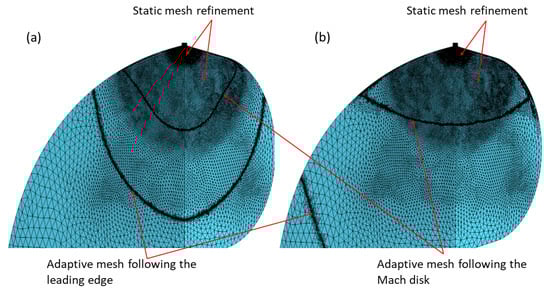
Figure 3.
Adaptive mesh after 7.0 ms (a) and 17.0 ms (b) of simulation.
4. Results
In this section, the main results of the 3D simulation are presented.
4.1. Flow Field
The jet start-up phase is shown in Figure 4. During the very first instants of expansion, the jet presents an almost planar front (see Figure 4a). This phase is quite short: after 0.5 ms of spreading, the jet begins to assume a spherical shape; see Figure 4b. The distinction between the first shock front (the leading edge) and the following one (the Mach disk) can be observed in Figure 4c, as expected in underexpanded jets [22,23]. Finally, the moment of the impact between the leading edge and the wall is shown in Figure 4f. Figure 5 shows the jet evolution after the impact on the VV inboard surface.
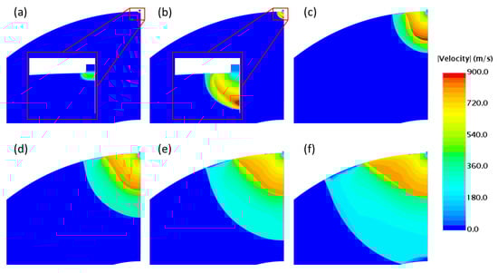
Figure 4.
Flow field evolution on the symmetry plane before the impact with the wall at (a) = 0.1 ms, (b) = 0.5 ms, (c) = 3.0 ms, (d) = 5.0 ms, (e) = 7.0 ms and (f) = 9.5 ms.
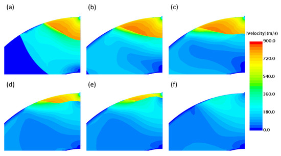
Figure 5.
Flow field evolution on the symmetry plane immediately after the impact with the wall at (a) = 11.0 ms, (b) = 17.0 ms, (c) = 25.0 ms, (d) = 40.0 ms, (e) = 45.0 ms and (f) = 55.0 ms.
The leading shock hits the wall first—see Figure 5a—causing the pressure on the wall surface to increase sharply—see Section 4.2. After the impact, a pressure wave starts to be reflected back, where it impacts on the Mach disk that is still propagating. As a consequence, the Mach disk starts to deform. In Figure 5a–c, the first spreading of the jet in the lateral direction is visible, as well as a shrinkage along the axial direction. Proceeding with the transient, the reflected wave strongly shrinks the Mach disk towards the inlet (see also Section 4.2), which completely dissipates around = 55.0 ms. This behaviour was not observed in the analysis of a He in-VV LOCA [15], and a systematic comparison of the two transients is reported below in Section 5.
The further evolution of the jet is shown in Figure 6. It can be seen that around = 170 ms, a second Mach disk starts developing (see Figure 6a–c), according to the characteristic features of an underexpanded jet [22,23]. However, due to the increase in the average pressure in the volume, the evolution of the second Mach disk is less violent than the first one and it stabilises at = 600 ms. The formation of a slipstream flowing away from the main jet can also be appreciated in Figure 6e,f, similar to that observed in [15]. From this moment on, the jet becomes almost steady; for this reason, no scalar scene after this time instant is presented, since they would not give any additional information. Moreover, according to [24], the Mach disk at = 600 ms, in steady-state conditions, should be located at 2.3 m from the pipe exit, which is very close to that shown in Figure 6f, in which the Mach disk is positioned at 2.7 m from the inlet. Note that this is a qualitative comparison only, in view of the different nature (transient vs. steady) of the phenomena.
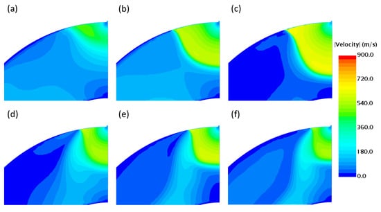
Figure 6.
Flow field evolution on the symmetry plane far after the impact with the wall at (a) = 170.0 ms, (b) = 200.0 ms, (c) = 270.0 ms, (d) = 310.0 ms, (e) = 400.0 ms and (f) = 590.0 ms.
4.2. Pressure Evolution and Phase Change
The pressure behaviour and the phase change are analysed during the transient, as the shock wave travels throughout the torus. The main objective is to monitor significant points; thus, the region near the inlet (point shown in Figure 7 as “Outboard”) and the one close to the front wall (point shown in Figure 7 as “Inboard”) are considered.
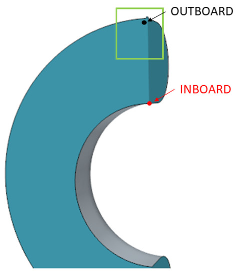
Figure 7.
Locations of the points used to monitor pressure and void fraction.
In Figure 8, the pressure evolution of the abovementioned points is presented. The first aspect that can be noticed is the peak in the “inboard” evolution, as already anticipated in Section 4.1, that causes a pressure increase from 0.1 bar to approximately 0.35 bar, which is not a concern regarding the structural integrity of the walls.
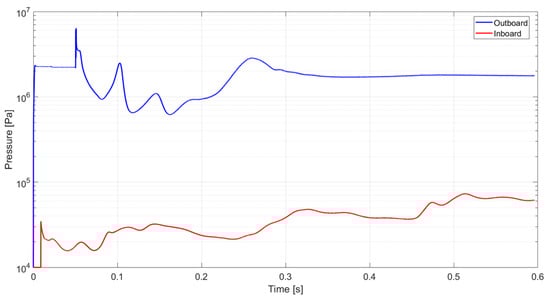
Figure 8.
Pressure evolution of “outboard” point (blue line) and “inboard” point (red line).
Proceeding with the transient, the region near the inlet is instead more relevant, as the reflected wave travels backwards. In Figure 9, it can be observed how the shock front, which corresponds to the local pressure peak, starts moving backwards after the impact (which occurs at 9.5 ms). Indeed, the peak shifts from ∼2.35 m to ∼2.5 m before the impact, while it moves from ∼2.0 m back to the pipe inlet afterwards (here, z is the coordinate along the jet axis).
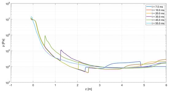
Figure 9.
Pressure profile along the symmetry axis at different time instants.
In order to provide a better understanding, the scalar map of the volume fraction of water shown in Figure 10 is reported only for the area highlighted in green in Figure 7.
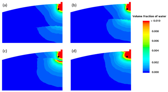
Figure 10.
Fraction of water with “outboard” point (black dot) superimposed on it, at (a) = 35.0 ms, (b) = 40.0 ms, (c) = 45.0 ms and (d) = 50.0 ms.
According to Figure 10, when the reflected wave reaches the inlet region, it starts compressing the Mach disk, causing a rapid increase of ∼44 bar in the “outboard” point (see Figure 8), as well as a significant increment in the liquid phase, as reported in Figure 11. Continuing to compress, the wave reaches the wall, where it causes the pressure to increase rapidly from ∼6 bar to ∼63 bar; a dedicated mechanical assessment should be performed in order to evaluate the effect of this fast pressure transient on the structure, which is, however, beyond the scope of this work.

Figure 11.
Volume fraction of water in correspondence with “outboard” point.
It is worth noticing that the pressure peak caused by the reflected wave is coherent with that expected in a water hammer event [25]. In particular, the pressure increase can be computed with the Joukowski equation, which is applicable also in the case of a two-phase mixture [26]:
where is the pressure variation across the discontinuity, K is equal to 0.5 in the event that the interaction of the wave is with a fluid, is the fluid density, c is the speed of sound and is the velocity variation across the discontinuity. Applying this formula on each of the discontinuities shown in Figure 9, agreement within 30% is found. This hints that the pressure peaks induced by the reflected pressure wave are physically consistent and that the phenomenon can be interpreted as a water hammer. Indeed, the inlet mass flow rate is strongly reduced as the first reflected wave reaches the inlet; see Figure 12.
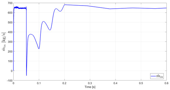
Figure 12.
Inlet mass flow rate evolution.
Successive pressure peaks are observed—see Figure 8—but, due to dissipation, these peaks are progressively lower than the first one and they gradually disappear.
It is worth highlighting that the reflected pressure wave—especially the first one—induces condensation at the wave front, as shown in Figure 10. This is a major difference with respect to single-phase jets and reflected waves—see, e.g., the helium jet analysed in [15]—since the condensation increases the observed pressure peak, because the transition from vapour to liquid strongly increases the density and, in turn, its compression leads to much higher pressure peaks than in a gas. This phenomenon shares some similarities with the so-called Condensation-Induced Water Hammer (CIWH) [27,28]. Although the CIWH is a concern if a single-phase liquid starts flowing in a saturated vapour section of a pipe, e.g., in nuclear fission reactors, some features of this phenomenon are also present in the case at hand. Indeed, the reflected pressure wave front is at high pressure, with a high fraction of liquid, and it comes into contact with a low-pressure, vapour volume. The latter condenses, thus reducing its volume and accelerating the liquid front further towards the inlet. Moreover, as observed in [27], the first pressure peak is the strongest, while the subsequent ones are progressively smaller, as also observed in the case at hand. However, the pressure peaks present in case of internal flows, as analysed in [27,28], are much larger than those observed in this work because, here, the flow is not strictly confined by a pipe. Nevertheless, the presence of the inboard wall acts as the closure of a valve in an internal flow, thus leading to a type of water hammer, with condensation on the wave front.
After the train of reflected pressure waves is dissipated, the flow at the inlet is restored, albeit leading to a less strong jet than the initial one, due to the increase in the average pressure in the volume, which in turn decreases the pressure ratio. Indeed, the pressure in “outboard” is lower than before the first pressure peak, and the same is true for the velocity at this point. This less strong jet is expected not to cause a reflected pressure wave as with the first one, and this is confirmed by the fact that the jet settles to a shape that is typical of steady underexpanded jets; see Figure 6.
Finally, the pressure of the wall located on the opposite side of the torus is considered, in order to asses when the burst disks will open (see Figure 13). The resulting analysis shows that the wave dissipates a lot of its energy while moving throughout the torus, causing then a relatively weak impact with the wall at = 68.0 ms. In particular, the pressure of the disks rises from 0.10 bar to 0.50 bar and then oscillates around the volume-averaged pressure for the rest of the transient. The latter is not affected by the pressure spikes induced by the waves and keeps rising very slowly for ∼2 s, when it reaches 1.5 bar, causing the opening of the BDs, thus concluding the time span simulated in this work. It is worth highlighting that the prediction of the pressurisation obtained with a system-level code (represented by the blue line in Figure 13) is conservative, since the computed pressure evolution is always above the one computed by CFD.
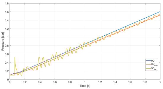
Figure 13.
Comparison of the evolution of the average pressure in the VV between 3D CFD model (red line) and 0D system-level code (blue line). The evolution of the the average pressure on the BD surface, as computed by CFD, is also reported (yellow line).
4.3. Temperature Field
The temperature field at different time instants is presented in Figure 14. Close to the inlet, the temperature remains almost constant; outside the inlet region, it rapidly decreases, reaching its minimum value in correspondence with the location where the fluid has the maximum velocity. Beyond this point, the temperature rapidly rises in the region characterised by the compression (shock front), and then decreases towards the wall.
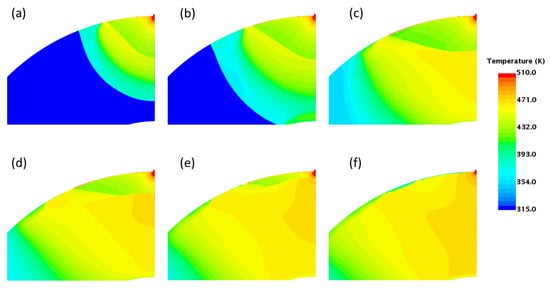
Figure 14.
Temperature distribution at (a) = 7.0 ms, (b) = 10.0 ms, (c) = 20.0 ms, (d) = 35.0 ms, (e) = 45.0 ms and (f) = 55.0 ms.
It is worth highlighting that the effects of the reflected wave, caused by the impact with the inboard wall, can be observed also in the temperature field evolution. In Figure 15, it is clear that (as discussed for the pressure), the shock front, i.e., where the “discontinuity” in the temperature profile can be observed, first moves towards the inboard wall (profiles at = 7.0 ms and = 10.0 ms) and then, after the impact, it is reflected back towards the inlet (profiles at = 20.0 ms and = 35.0 ms). The progressive (global) increase in temperature with time can also be noticed in both figures.
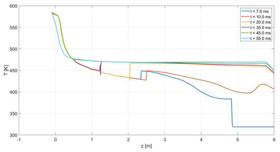
Figure 15.
Temperature profile along the symmetry axis at different time instants.
5. Comparison with the Helium-Cooled BB Case
The WCLL is one of the two alternative BB concepts considered within the EU DEMO project [6,29], the other one being a helium-cooled concept (the Helium-Cooled Pebble Bed, HCPB) [30]. While the present work focuses on an in-vessel LOCA caused by a failure in a water-cooled BB, an analogous case for a helium-cooled BB has been published in [15]. In the current status of the HCPB design, the helium coolant enters at a nominal pressure of 8 MPa and with a nominal temperature range of 300–520 °C.
The main difference between the helium jet and the water jet is that the helium does not undergo a phase change; thus, it is not characterised by the flashing mechanism. On the contrary, it behaves as a highly under-expanded single-phase jet. Being a single-phase gas, the helium expands inside the vessel at hypersonic velocity, impacting on the opposite wall in less than 2.5 ms. This means that the leading shock is still very strong when it reaches the wall (i.e., it has a greater amount of energy), causing a more violent impact with the inboard surface. This is also due to the fact that the helium jet develops mainly along the axial direction, so it dissipates less energy. On the contrary, for the water case, the vapour enters the vessel at a much lower velocity due to the flashing phenomenon, allowing the flow to expand in all directions and taking around 9.5 ms to reach the opposite wall. The energetic content of the jet has a direct impact on the pressure spike experienced by the walls. Indeed, the pressure reached on the front wall after the impact with the leading edge has approximately one order of magnitude of difference between the two cases. In particular, in the helium transient, 3.5 bar is reached, while, in the water analysis, the pressure reaches 0.35 bar. Furthermore, the water jet gives rise to a strong reflected wave that deforms significantly the Mach disk while moving backwards. The condensation induced on the wave front allows the wave to completely dissipate the Mach disk and to reach the outboard wall, where it generates a pressure spike of 63 bar. On the contrary, the reflected wave generated in the helium case is not strong enough to dissipate completely the Mach disk, which is much stronger than that of water, and so it cannot reach the outboard wall.
The different expansion mechanisms of the two jets cause also the temperatures reached during the transient to be very different: for the helium setup, both very high (∼1500 K) and very low (∼30 K) temperatures are reached, while, in the case of water, the temperature is always between 290 K and 600 K.
6. Conclusions and Perspective
A model to simulate the coolant behaviour following an in-vessel Loss-of-Coolant Accident in a tokamak fusion reactor, causing a break in a water-cooled First Wall, has been developed using a CFD approach. The model represents an extension of a model previously developed for a helium-cooled FW, taking into account the additional complications deriving from the flash boiling happening when pressurised water is released inside the vacuum vessel.
The 3D model is able to resolve the different shocks forming when the high-pressure water is suddenly exposed to the low-pressure VV environment, also thanks to the Adaptive Mesh Refinement algorithm, which progressively refines and coarsens the mesh to follow the front propagation. Such a model allows an evaluation of local pressure peaks on the walls, enabling a detailed mechanical assessment of its integrity, according to the (local) failure criteria set for the VV.
The results highlight that the pressure peak on the wall in front of the break is much weaker than in the case of a single-phase coolant release, but the wave reflection, combined with the condensation effects, causes a steep pressure increase on the wall close to the rupture itself. Similarly, the evolution of the pressure on the opposite side of the chamber, where the safety burst disks are assumed to be located, is much smoother than in the case of a helium-cooled FW, following in broad terms the evolution of the average pressure in the chamber. A comparison with a 0D model confirms that, as far as the pressure on the BD and the timing for their opening are concerned, a 0D analysis is sufficient to have a good estimate. The same may not hold true if the aim is to assess the failure of the containment, which is based on local criteria.
In perspective, some of the model’s simplifying assumptions are planned to be addressed, particularly concerning the geometry, as well as the initial part of the transient, which cannot be simulated with a CFD model.
Author Contributions
Conceptualisation, A.F. and A.Z.; methodology, M.S., A.F. and A.Z.; software, M.S.; validation, M.S. and A.Z.; resources, A.F. and A.Z.; data curation, M.S.; writing—original draft preparation, M.S.; writing—review and editing, A.F. and A.Z.; visualisation, M.S.; supervision, A.F. and A.Z.; funding acquisition, A.F. and A.Z. All authors have read and agreed to the published version of the manuscript.
Funding
This work has been carried out within the framework of the EUROfusion Consortium, funded by the European Union via the Euratom Research and Training Programme (Grant Agreement No 10105220 – EUROfusion). Views and opinions expressed are however those of the author(s) only and do not necessarily reflect those of the European Union or the European Commission. Neither the European Union nor the European Commission can be held responsible for them. The work of A. Zappatore is financially supported by a EUROfusion Researcher Grant. The APC was partially funded by Politecnico di Torino through the Open Access initiative.
Data Availability Statement
The data presented in this study are available on request from the corresponding author.
Conflicts of Interest
The authors declare no conflict of interest. The funders had no role in the design of the study; in the collection, analyses, or interpretation of data; in the writing of the manuscript; or in the decision to publish the results.
Appendix A. Model Development and Validation
The model developed in this work is validated against the results presented in [31]. This work is selected as a benchmark because of its similarity with the configuration of interest for this work: it presents a simple computational domain—see Figure A1—and uses pressurised sub-cooled water as a working fluid, which undergoes flash boiling at the exit of the pipe. Even though the selected transient is 2D, with a much smaller pressure ratio than that analysed for the EU DEMO-relevant scenario, it should allow us to test all the relevant models needed for the more complex 3D case.

Figure A1.
Computational domain and boundary conditions of the simple 2D case.
Figure A1.
Computational domain and boundary conditions of the simple 2D case.

Appendix A.1. Setup
The boundary conditions are listed below, with reference to Figure A1.
- Inlet: stagnation inlet with fixed supersonic pressure, total pressure and total temperature.
- Outlet: pressure outlet with fixed pressure and temperature.
- Bottom boundary: symmetry plane.
- Walls: no slip condition.
The initial conditions are reported in Table A1.

Table A1.
Initial conditions of the 2D transient simulation.
Table A1.
Initial conditions of the 2D transient simulation.
| pin [MPa] | Tin [K] | |
|---|---|---|
| Water | 5.0 | 519.1 |
| Vapour | 0.1 | 372.8 |
Appendix A.2. Model
The list of the adopted models is as follows:
- (a)
- 2D
- (b)
- Implicit unsteady
- (c)
- Turbulent (realisable two-layer)
- (d)
- Multiphase
- (e)
- Volume of Fluid (VOF)
- (f)
- Segregated flow
- (g)
- Segregated multiphase temperature
Regarding the mesh settings, a tetrahedric static mesh is used since the built-in AMR solver can be applied only on 3D problems.
Appendix A.3. Results
The simulation results are compared against the solutions proposed by Minato et al. in [31]. The evolution of the two-phase flow is analysed throughout the transient, reporting the graphical results for three time instants: 1, 10 and 40 ms, respectively. The paper does not provide numerical data, so the comparison is performed graphically, in a qualitative manner.
In Figure A2, a comparison of the void fraction distributions is shown. The fluid starts flashing at the pipe exit, generating an interface between the water and the two-phase mixture that travels towards the vessel walls. As the interface keeps travelling, a vapour annulus starts forming in correspondence with the inlet section at 10 ms. Then, at 40 ms, the interface reaches the pipe inlet, generating a conical liquid core.

Figure A2.
Void fraction comparison. Minato et al. [31] (left), this work (right).
Figure A2.
Void fraction comparison. Minato et al. [31] (left), this work (right).

Figure A3 presents the pressure field comparison. The numerical solution shows good agreement with the results published in [31]. In particular, the pressure distribution has the same structure already seen for the void fraction, with a high-pressure core and a lower-pressure annulus. In addition, the solution shows a classic flashing jet behaviour, where the volume expansion caused by the rapid evaporation of the liquid prevents the over-depressurisation of the two-phase mixture inside the pipe.
The velocity fields for the two phases are reported in Figure A4 and Figure A5. The gas velocity field at 1 ms shows the initial flashing of the vapour followed by the expansion of the flow structure. In the water velocity field, instead, one can observe a progressive acceleration from 10 ms to 40 ms. The model performs quite well, giving satisfactory agreement with the results reported in [31].

Figure A3.
Pressure comparison. Minato et al. [31] (left), this work (right).
Figure A3.
Pressure comparison. Minato et al. [31] (left), this work (right).


Figure A4.
Water velocity profile comparison. Minato et al. [31] (left), this work (right).
Figure A4.
Water velocity profile comparison. Minato et al. [31] (left), this work (right).


Figure A5.
Vapour velocity profile comparison. Minato et al. [31] (left), this work (right).
Figure A5.
Vapour velocity profile comparison. Minato et al. [31] (left), this work (right).

Given that all the results have a good level of agreement with the ones of the reference case, the adopted models can be considered reliable and they can be applied to the 3D transient case.
References
- Donné, A.J.H.; Morris, W.; Litaudon, X.; Hidalgo, C.; McDonald, D.; Zohm, H.; Diegele, E.; Möslang, A.; Nordlund, K.; Federici, G.; et al. European Reasearch Roadmap to the Realisation of Fusion Energy; EUROfusion Consortium: Garching, Germany, 2018; ISBN 978-3-00-061152-0. [Google Scholar]
- Federici, G.; Baylard, C.; Beaumont, A.; Holden, J. The plan forward for EU DEMO. Fusion Eng. Des. 2021, 173, 112960. [Google Scholar] [CrossRef]
- Federici, G.; Holden, J.; Baylard, C.; Beaumont, A. The EU DEMO staged design approach in the Pre-Concept Design Phase. Fusion Eng. Des. 2021, 173, 112959. [Google Scholar] [CrossRef]
- Caruso, G.; Ciattaglia, S.; Colling, B.; Di Pace, L.; Dongiovanni, D.L.; D’Onorio, M.; Garcia, M.; Jin, X.Z.; Johnston, J.; Leichtle, D.; et al. DEMO—The main achievements of the Pre–Concept phase of the safety and environmental work package and the development of the GSSR. Fusion Eng. Des. 2022, 176, 113025. [Google Scholar] [CrossRef]
- Froio, A.; Moscato, I. Effect of different system parameters on the design of the EU DEMO Vacuum Vessel Pressure Suppression System. Fusion Eng. Des. 2023, 190, 113543. [Google Scholar] [CrossRef]
- Spagnuolo, G.A.; Arredondo, R.; Boccaccini, L.V.; Chiovaro, P.; Ciattaglia, S.; Cismondi, F.; Coleman, M.; Cristescu, I.; D’Amico, S.; Day, C.; et al. Integrated design of breeding blanket and ancillary systems related to the use of helium or water as a coolant and impact on the overall plant design. Fusion Eng. Des. 2021, 173, 112933. [Google Scholar] [CrossRef]
- Ahn, M.Y.; Cho, S.; Kim, D.H.; Lee, E.S.; Kim, H.S.; Suh, J.S.; Yun, S.; Cho, N.Z. Preliminary safety analysis of Korea Helium Cooled Solid Breeder Test Blanket Module. Fusion Eng. Des. 2008, 83, 1753–1758. [Google Scholar] [CrossRef]
- D’Onorio, M.; D’Amico, S.; Froio, A.; Porfiri, M.T.; Spagnuolo, G.A.; Caruso, G. Benchmark analysis of in-vacuum vessel LOCA scenarios for code-to-code comparison. Fusion Eng. Des. 2021, 173, 112938. [Google Scholar] [CrossRef]
- Nakamura, M.; Tobita, K.; Someya, Y.; Utoh, H.; Sakamoto, Y.; Gulden, W. Thermohydraulic responses of a water-cooled tokamak fusion DEMO to loss-of-coolant accidents. Nucl. Fusion 2015, 55, 123008. [Google Scholar] [CrossRef]
- D’Onorio, M.; Giannetti, F.; Porfiri, M.T.; Caruso, G. Preliminary safety analysis of an in-vessel LOCA for the EU-DEMO WCLL blanket concept. Fusion Eng. Des. 2020, 155, 111560. [Google Scholar] [CrossRef]
- Porfiri, M.; Meloni, P. Post-test calculations with ISAS-ITER system for ICE experiments. In Proceedings of the 19th IEEE/IPSS Symposium on Fusion Engineering, 19th SOFE (Cat. No.02CH37231), Atlantic City, NJ, USA, 25 January 2002; pp. 48–51. [Google Scholar] [CrossRef]
- Caruso, G.; Bartels, H.; Iseli, M.; Meyder, R.; Nordlinder, S.; Pasler, V.; Porfiri, M. Simulation of cryogenic He spills as basis for planning of experimental campaign in the EVITA facility. Nucl. Fusion 2005, 46, 51. [Google Scholar] [CrossRef]
- Froio, A.; Bertinetti, A.; Ciattaglia, S.; Cismondi, F.; Savoldi, L.; Zanino, R. Modelling an in-vessel loss of coolant accident in the EU DEMO WCLL breeding blanket with the GETTHEM code. Fusion Eng. Des. 2018, 136, 1226–1230. [Google Scholar] [CrossRef]
- Froio, A.; Barucca, L.; Ciattaglia, S.; Cismondi, F.; Savoldi, L.; Zanino, R. Analysis of the effects of primary heat transfer system isolation valves in case of in-vessel loss-of-coolant accidents in the EU DEMO. Fusion Eng. Des. 2020, 159, 111926. [Google Scholar] [CrossRef]
- Zappatore, A.; Froio, A.; Spagnuolo, G.A.; Zanino, R. 3D transient CFD simulation of an in-vessel loss-of-coolant accident in the EU DEMO fusion reactor. Nucl. Fusion 2020, 60, 126001. [Google Scholar] [CrossRef]
- Arena, P.; Del Nevo, A.; Moro, F.; Noce, S.; Mozzillo, R.; Imbriani, V.; Giannetti, F.; Edemetti, F.; Froio, A.; Savoldi, L.; et al. The DEMO Water-Cooled Lead-Lithium Breeding Blanket: Design Status at the End of the Pre-Conceptual Design Phase. Appl. Sci. 2021, 11, 11592. [Google Scholar] [CrossRef]
- Gliss, C. DEMO Reference Configuration Model; EFDA_D_2MUNPL; EUROfusion Consortium: Garching, Germany, 2017. [Google Scholar]
- Siemens Digital Industries Software. Simcenter STAR-CCM+ User Guide v. 2021.2; Siemens: Munich, Germany, 2021. [Google Scholar]
- Jin, X.Z. BB LOCA analysis for the reference design of the EU DEMO HCPB blanket concept. Fusion Eng. Des. 2018, 136, 958–963. [Google Scholar] [CrossRef]
- Froio, A.; Bertinetti, A.; Savoldi, L.; Zanino, R.; Cismondi, F.; Ciattaglia, S. Benchmark of the GETTHEM Vacuum Vessel Pressure Suppression System (VVPSS) model for a helium-cooled EU DEMO blanket. In Proceedings of the 27th European Safety and Reliability Conference on Safety and Reliability—Theory and Applications, Portorož, Slovenia, 18–22 June 2017; pp. 59–66. [Google Scholar] [CrossRef]
- De Lorenzo, M.; Lafon, P.; Di Matteo, M.; Pelanti, M.; Seynhaeve, J.M.; Bartosiewicz, Y. Homogeneous two-phase flow models and accurate steam-water table look-up method for fast transient simulations. Int. J. Multiph. Flow 2017, 95, 199–219. [Google Scholar] [CrossRef]
- Shapiro, A.H. The Dynamics and Thermodynamics of Compressible Fluid Flow; Wiley: New York, NY, USA, 1953; Volume 1. [Google Scholar]
- Anderson, J.D. Modern Compressible Flow with Historical Perspective, 3rd ed.; McGraw-Hill: New York, NY, USA, 2003. [Google Scholar]
- Franquet, E.; Perrier, V.; Gibout, S.; Bruel, P. Free underexpanded jets in a quiescent medium: A review. Prog. Aerosp. Sci. 2015, 77, 25–53. [Google Scholar] [CrossRef]
- Ghidaoui, M.S.; Zhao, M.; McInnis, D.A.; Axworthy, D.H. A Review of Water Hammer Theory and Practice. Appl. Mech. Rev. 2005, 58, 49–76. [Google Scholar] [CrossRef]
- Griffith, P. Screening Reactor Steam/Water Piping Systems for Water Hammer; Technical Report; OSTI: Washington, DC, USA, 1997. [CrossRef]
- Barna, I.F.; Imre, A.R.; Baranyai, G.; Ézsöl, G. Experimental and theoretical study of steam condensation induced water hammer phenomena. Nucl. Eng. Des. 2010, 240, 146–150. [Google Scholar] [CrossRef]
- Datta, P.; Chakravarty, A.; Ghosh, K.; Mukhopadhyay, A.; Sen, S.; Dutta, A.; Goyal, P.; Thangamani, I. Modeling and analysis of condensation induced water hammer. Numer. Heat Transf. Part A Appl. 2018, 74, 975–1000. [Google Scholar] [CrossRef]
- Boccaccini, L.; Arbeiter, F.; Arena, P.; Aubert, J.; Bühler, L.; Cristescu, I.; Nevo, A.D.; Eboli, M.; Forest, L.; Harrington, C.; et al. Status of maturation of critical technologies and systems design: Breeding blanket. Fusion Eng. Des. 2022, 179, 113116. [Google Scholar] [CrossRef]
- Hernández, F.A.; Pereslavtsev, P.; Zhou, G.; Kang, Q.; D’Amico, S.; Neuberger, H.; Boccaccini, L.V.; Kiss, B.; Nádasi, G.; Maqueda, L.; et al. Consolidated design of the HCPB Breeding Blanket for the pre-Conceptual Design Phase of the EU DEMO and harmonization with the ITER HCPB TBM program. Fusion Eng. Des. 2020, 157, 111614. [Google Scholar] [CrossRef]
- Minato, A.; Takamori, K.; Suzuki, A. Numerical Study of Two-Dimensional Structure in Critical Steam-Water Two-Phase Flow. J. Nucl. Sci. Technol. 1995, 32, 464–475. [Google Scholar] [CrossRef]


Disclaimer/Publisher’s Note: The statements, opinions and data contained in all publications are solely those of the individual author(s) and contributor(s) and not of MDPI and/or the editor(s). MDPI and/or the editor(s) disclaim responsibility for any injury to people or property resulting from any ideas, methods, instructions or products referred to in the content. |
© 2023 by the authors. Licensee MDPI, Basel, Switzerland. This article is an open access article distributed under the terms and conditions of the Creative Commons Attribution (CC BY) license (https://creativecommons.org/licenses/by/4.0/).