Abstract
Accurately predicting well productivity is crucial for optimizing gas production and maximizing recovery from tight gas reservoirs. Machine learning (ML) techniques have been applied to build predictive models for the well productivity, but their high complexity and low interpretability can hinder their practical application. This study proposes using interpretable ML solutions, SHapley Additive exPlanations (SHAP) and Local Interpretable Model-agnostic Explanations (LIME), to provide explicit explanations of the ML prediction model. The study uses data from the Eastern Sulige tight gas field in the Ordos Basin, China, containing various geological and engineering factors. The results show that the gradient boosting decision tree model exhibits superior predictive performance compared to other ML models. The global interpretation using SHAP provides insights into the overall impact of these factors, while the local interpretation using SHAP and LIME offers individualized explanations of well productivity predictions. These results can facilitate improvements in well operations and field development planning, providing a better understanding of the underlying physical processes and supporting more informed and effective decision-making. Ultimately, this study demonstrates the potential of interpretable ML solutions to address the challenges of forecasting well productivity in tight gas reservoirs and enable more efficient and sustainable gas production.
1. Introduction
China’s reserves of onshore tight gas are substantial, with an estimated more than 20 trillion m3 of proven reserves as of 2021 [1,2]. The applications of hydraulic fracturing technology have facilitated the extraction of the natural gas, and accounted for approximately 24.4% of China’s total natural gas production in 2020, which amounted to 47 billion m3 [3]. The Ordos Basin in western China has experienced significant growth in the tight gas production over the past decade, with several giant gas fields having more than 4 trillion m3 reserves. Notably, the Sulige stands out as the largest tight gas-producing field in China, with proven natural gas reserves of more than 600 billion m3 [4,5].
Accurate well productivity forecasting (WPF) is crucial for the effective evaluation and development of the tight gas fields as the productivity is closely linked to optimizing hydraulic fracturing design, well spacing, and investment decision-making. However, due to the complex pore structure and intricate transport mechanisms of natural gas in the tight formations, flow mechanisms remain insufficiently understood. Therefore, the WPF has been a significant subject of research for the tight gas reservoirs. Several predictive methods have been proposed and can be classified according to the degree of reliance on physical information and the necessary data for modeling [6]. The mechanistic method, which leverages the underlying physics, builds rigorous mathematical models that describe the complex physical phenomena during natural gas extraction from the tight formations [7,8,9,10]. The model parameters are built upon the physical concepts. Consequently, the mechanistic models offer plausible explanations for the physical phenomena and have strong generalization ability due to their strict adherence to the first principle [11].
Analytical and reservoir simulation methods are two examples of mechanistic modeling techniques used in the WPF. Most analytical methods rely on idealized assumption such as homogeneous reservoirs, single-phase flow, and simple fracture geometries, to derive analytical equations for the well productivity [12,13,14]. However, these simplifications may lead to significant predictive errors, particularly in heterogeneous reservoirs with complex fracture networks and multi-phase flow. For the scenario, reservoir simulation method can achieve reasonable results by simulating the flow processes of oil, gas, and water phases through the tight matrix and fracture networks. Even so, accurately characterizing underlying flow mechanisms in nanoscale and micro-scale pores presents challenges to the simulation method. For example, traditional Darcy’s law may be insufficient in these cases. In addition, the effectiveness of the reservoir simulation relies upon correct reservoir characterization and time-consuming history matching results [15,16,17]. The simulations usually require the utilization of fine-scale grids and iterative solutions of the partial differential equations of multiphase flow, which lead to computationally expensive and time-consuming. Thus, the reservoir simulation method cannot meet the time-efficient demand of tight gas field development. In summary, the problems have limited the application and promotion of the mechanistic models in the real gas fields.
The advancement of artificial intelligence (AI) technology, coupled with the increasing availability of data resulting from rapid gas field development, has shown significant potential in the development of machine learning (ML) models for the WPF [18,19]. Such models are particularly effective in addressing the complex problems, particularly when the current seepage theory is not mature enough to accurately model the gas flow behavior. The data-driven approach enables the capture of intricate nonlinear relationships between fractured well productivity and various contributing factors, such as formation properties, drilling and completion procedures, and fracturing treatments. Compared with the mechanistic models, the ML algorithms require only historical data instead of detailed physical information, making them easier to develop and apply. Various supervised learning algorithms, such as support vector machines (SVM), decision trees (DT), artificial neural networks (ANN), and ensemble learning such as random forest (RF) and gradient boosting decision tree (GBDT), have been investigated for the WPF as shown in Table 1.

Table 1.
Machine learning algorithms to predict well productivity.
The predictive performances of the developed models exhibit a high level of accuracy, as evidenced by the coefficient of determination (R2) on the testing data sets in Table 1. In addition to high prediction performance, a significant advantage of the data-driven approach is its speed of prediction. Once the predictive models are successfully built, the predictions can be made within a matter of seconds. This allows for timely decision-making in the tight gas field development where many wells need to be drilled and then stimulated.
Although the applications of ML algorithms have demonstrated considerable potential for enhancing the efficiency and reliability of the WPF, the lack of interpretability in these “black box” models has hindered petroleum engineers from understanding the rationale behind the model prediction. In addition to knowing the productivity of the fractured wells from the models, it is also crucial for the engineers to know how the primary parameters impact the well productivity to improve hydraulic fracturing design and well spacing. Further, it is also essential to investigate the degree of influence of each feature on an individual well productivity prediction to identify potential errors or biases. Unfortunately, previous ML applications offer little insight into the rationale behind the prediction outcomes at both global and local levels. It is, therefore, necessary to improve model interpretability to enhance the applicability of the ML techniques in the WPF.
Recent studies have focused on interpretability to comprehend how ML models learn from data, the learned patterns, and how they generate specific predictions [26,27]. In this research, we utilized three supervised ML algorithms to predict the well productivity in the Eastern Sulige gas field. Furthermore, the study employed Shapley additive explanations (SHAP) and local interpretable model-agnostic explanations (LIME) techniques to reveal the important features and provide an underlying rationale for the prediction results at the global and local levels. These approaches are described in Section 3.
2. Data Preparation
The study utilized data obtained from the hydraulically fractured vertical wells in the Eastern Sulige gas field, which is situated in the Ordos basin, China (see Figure 1).
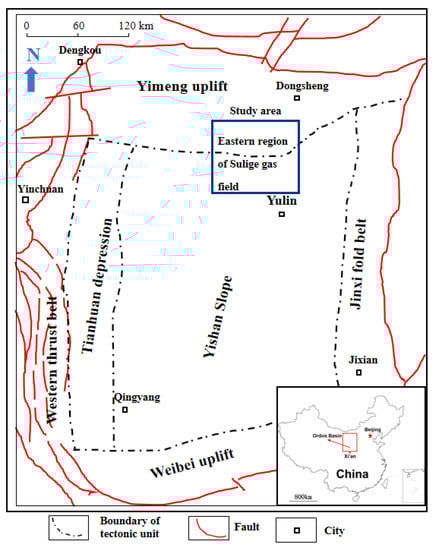
Figure 1.
The study area in the Sulige gas field.
The gas field spans an exploration area of 11,000 km2, stretching from the Ordos district in the Inner Mongolia autonomous region to the Yulin district of Shaanxi province, China. The primary producing zone in the study area is the He8 Member of the lower Shihezi formation, which consists of multiple and thin gas-bearing layers, with thicknesses ranging from 20 m to 60 m. The lithology of the formation is sandstone of the fluvial-delta facies, with strong heterogeneity. The average matrix porosity is between 4% to 12%, and the average matrix permeability ranges from 0.01 mD to 1 mD. The average depth of the gas reservoirs in the northern and southern parts of the study area varies from 2500 m to 3300 m [28]. Since 2010, more than 2000 wells have been drilled and put into production in the Shihezi Formation, with vertical wells accounting for over 80% of the total number of fractured wells [29].
The study involved the collection of production data from more than 700 fractured vertical wells operated by different departments. The productivity of these gas wells is quantified using absolute open flow potential (AOFP), a common indicator of well productivity. The well AOFP is usually determined with a one-point well test method that is widely employed in the Chinese gas field. Three types of important features that affect the AOFP were investigated including geological properties of the formation, well test constraints and fracturing treatment parameters. Each of the fractured vertical wells includes 18 input features. Table 2 summarizes the statistical properties of the response variable and the selected features.
Table 2.
Statistical properties of input and target variables used in the study.
3. Methodology
3.1. Workflow of Developing Interpretable ML Models
The workflow for developing interpretable ML models is presented in Figure 2 and involves four main steps.
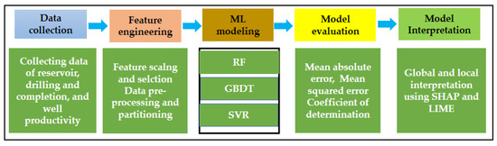
Figure 2.
Workflow for developing interpretable ML models for this study.
In Step 1, the raw data gathered from the study area is transformed into a dataset suitable for ML applications. The data types and statistical characteristics of the collected data have been shown in Table 1.
In Step 2, feature engineering is a crucial step in developing effective ML models. The model performances are largely determined by the quality and relevance of the features. Feature engineering includes data cleaning and preprocessing, feature scaling and selection. In data cleaning and preprocessing, the raw data are preprocessed for predictive modeling through the removal of inconsistent data points and the handling of missing values and outliers. The details of the data preprocessing in this investigation were discussed in a previous study [30].
In Step 3, a multitude of ML algorithms are available in the literature. Nonetheless, each algorithm possesses its own strengths and weaknesses, and may be better suited for certain problems. Hence, it is imperative to compare multiple ML models and determine the most effective one for each study. Random forest (RF), support vector regression (SVR), and gradient boosting decision tree (GBDT) were employed to address complex regression problems in WPF.
In Step 4, the evaluation of each established model is carried out to determine the most accurate model, which can then be utilized for model interpretability. Three commonly adopted statistical metrics, namely the coefficient of determination (R2), mean squared error (MSE), and mean absolute error (MAE) are selected for this purpose. The calculations of these metrics are based on the following formulas:
where n signifies the number of data points, and represent the ith observed and predicted target values, respectively, and denotes the mean value of the observed target data. The coefficient of determination ranges from 0 to 1, with higher values indicating better performance. Conversely, smaller values of MSE and MAE correspond to higher accuracy levels.
Finally, in Step 5, the chosen model from the preceding step is explained through the SHAP and LIME methods to provide insights into how the model makes predictions globally and locally, thereby facilitating a deeper understanding of the model’s prediction process. This step is crucial as it provides valuable information for optimal hydraulic fracturing design to maximize gas recovery.
3.2. Predictive Model Building
We developed black-box models for evaluating the productivity of fractured wells by employing three powerful machine learning algorithms, namely Support Vector Regression (SVR), Random Forest (RF), and Gradient Boosting Decision Tree (GBDT). The following subsections provide a brief theoretical background of these algorithms.
3.2.1. Random Forest
Random forest (RF) is an ensemble method that is composed of multiple decision trees, which are constructed using both bootstrapped samples from a training set and feature bagging [31]. The approach of using an ensemble of decision trees in the RF algorithm allows it to improve the predictive performance of a single decision tree. Furthermore, the RF model has the advantage of preventing overfitting and reducing variance by aggregating the output of multiple decision trees. For regression problems, the output of a RF model is the average of individual decision tree outputs. To train the RF model, several tuning parameters must be specified, including the number of decision trees to grow in the RF (N_estimators), the number of randomly defined predictor variables at each node when searching for the best split (Max_features), and the minimum number of observations required to split an internal node (min_samples_split) [32]. In this study, the RF predictive model was developed using the Scikit-Learn package in Python [32].
Random Forest is well-suited for handling high-dimensional data since it employs a technique that randomly selects subsets of features for each split, reducing the risk of overfitting. Furthermore, it can efficiently handle large datasets with a high number of input features and can produce results in a reasonable amount of time. Additionally, the model can handle both continuous and categorical features and can identify the most important features for prediction.
3.2.2. Gradient Boosting Decision Tree
Gradient boosting decision tree (GBDT) is an also ensemble learning algorithm that belongs to the family of boosting algorithms by combining multiple decision trees sequentially [33]. GBDT works by iteratively adding decision trees to the ensemble, where each subsequent tree is built to correct the errors made by the previous trees. The algorithm starts with a simple decision tree, and then the subsequent trees are added and trained on the residuals of the previous trees. The residuals are the differences between the true values and the predicted values of the previous trees.
The prediction of the ensemble of decision trees can be written as:
where F(x) is the predicted value for a given input x, M is the total number of decision trees in the ensemble, and fm(x) is the prediction of the mth decision tree.
A loss function measures the difference between the predicted values and the true values, and can be written as:
where N is the total number of training samples, yi is the true label of the ith training sample, F(xi) is the predicted value for the ith training sample, and r(yi, F(xi)) is the loss function for the ith training sample. This training process continues until a predefined stopping criterion is met, such as the maximum number of trees to be created. Most tuning hyperparameters used for RF are applied for GBDT as well.
GBDT is a widely recognized machine learning algorithm for its high predictive accuracy, particularly due to its capacity to model complex non-linear relationships between variables. This algorithm also has the ability to handle missing data efficiently and can process different types of data, including numerical and categorical variables. This versatility makes GBDT a useful tool for various applications. Additionally, GBDT automatically performs feature selection by assigning higher importance to the most relevant features, which can improve the overall accuracy of the model. In contrast, random forest, gives equal importance to all features, which can result in lower accuracy when dealing with datasets containing irrelevant features.
3.2.3. Support Vector Regression
Support Vector Regression (SVR) is a regression method based on support vector machines that construct two separating hyperplanes on either side of a regression function. Given a set of training data where xi is a multivariate set of M observations with corresponding response values yi, SVR constructs a nonlinear function f(x) that can be expressed as follows [34,35]:
Subject to:
where C is the box constraint that controls the penalty imposed on observations that lie outside the epsilon margin (ε) and helps to prevent overfitting (regularization). and are the slack variables that provide the lowest and highest range training errors, respectively. In this study, the radial basis function (RBF) kernel was used to construct the SVR model, which can be expressed as follows:
where γ is a parameter that sets the spread of the kernel.
SVR is a suitable method for high-dimensional datasets where the number of features significantly exceeds the number of samples. This is because SVR considers only the support vectors, which are the samples closest to the decision boundary, and disregards the remaining samples. Additionally, SVR can handle non-linear data by utilizing a non-linear kernel function, allowing it to capture complex patterns in the data. Another advantage of SVR is its ability to handle outliers, as it is relatively insensitive to data points that do not lie near the decision boundary. However, SVR may not perform well when dealing with datasets that have many samples, as the computational cost can become prohibitive in solving a quadratic optimization problem.
3.3. Model Interpretability
Model interpretability refers to the degree to which the predictions of a ML model can be understood by a human [25]. In recent years, various interpretable ML techniques have been proposed. These techniques can be classified into different groups based on application stage, interpretability scope, and model dependency as illustrated in Figure 3 [36,37].
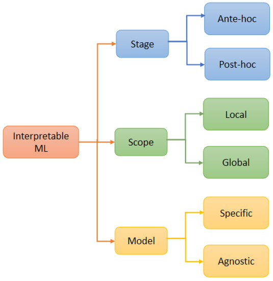
Figure 3.
Classification of interpretable ML methods (modified from [36,37]).
3.3.1. Scope
Interpretability scope refers to the range of black-box ML model output that needs to be interpreted, which can be at a global or local level. At the global level, interpretation is made based on a full view of the model structures and parameters, providing a holistic understanding by estimating the global effects of input features on model predictions. This requires both the black-box model and the entire training data. In the context of WPF, global interpretability is essential for explaining which features are most significant in controlling well productivity. On the other hand, local interpretability focuses on a single prediction or a group of predictions to investigate how the predictions are made. Both the black-box model and the prediction values are needed. Local interpretation is crucial to trust the predictions. For example, local interpretability can help explain how the input features contribute to the well productivity.
Some techniques can provide both local and global interpretation, such as Shapley additive explanations (SHAP), while local interpretable model-agnostic explanations (LIME) obtain local interpretation for individual predictions by building local surrogate models. The details of these methods are described in the next subsection.
3.3.2. Dependency
Model dependency pertains to the extent to which an interpretable technique can be utilized on any ML model or specific models. Certain interpretation techniques consider ML models as black-box models and are thereby applicable to any model, thus qualifying as model-agnostic techniques. Conversely, other techniques are model-specific, as they can only be employed for the interpretation of certain ML models. Model-agnostic techniques require solely the input and output of the ML model, disregarding its inner structures, thus enabling their application to any ML model. In contrast, model-specific techniques can investigate the specific characteristics or architecture of the ML model, providing detailed interpretability that may not be attainable with model-agnostic methods.
3.3.3. Stage
Interpretable ML techniques can also be categorized into ante-hoc and post-hoc methods based on when they are employed in the model building process. Ante-hoc interpretable techniques involve using algorithms with high transparency during the training process, resulting in a model that is inherently interpretable. For example, linear regression is an ante-hoc model since the coefficients of the linear model can be interpreted as the extent of influence of individual features on the prediction [25]. However, this approach may result in models that are overly simplistic and have inadequate prediction accuracy. In contrast, post-hoc interpretable ML techniques are applied to established models after the training process.
3.4. Shapley Additive Explanations (SHAP)
SHAP is a post-hoc interpretive tool that was introduced by Lundberg and Lee in 2017 [38]. This technique is designed to facilitate the interpretation of the output generated by any ML model. SHAP is based on the concept of Shapley value and has a strong foundation in cooperative game theory. The computation of the Shapley value for each feature is based on a conditional expectation function, which allows for the representation of the feature’s marginal contribution. By calculating the Shapley value for each input feature, SHAP provides an interpretation of the model’s predicted values as the sum of the Shapley values, as given by Equation (9):
where, f(x*) is ML predicted value, 0 is average prediction for the training dataset, and is the Shapley value for a feature j.
The SHAP technique allows for both global and local explanations of ML models. Global explanations summarize the impact of each feature across the entire dataset, while local explanations identify the impact of each feature for a specific instance or subset of instances. In this study, we employed the SHAP Python package, which is compatible with tree-based models from the scikit-learn machine learning library. The package includes visualization tools such as summary plots and dependence plots, which aid in improving the interpretability of the ML models.
Local Interpretable Model-Agnostic Explanations (LIME)
LIME was introduced by Ribeiro et al. in 2016 as a model-agnostic approach to obtaining local interpretations for individual predictions [39]. Given an instance x and a black-box model f, LIME generates an interpretable model g(x) that approximates prediction f(x) in a local neighborhood of x. The local neighborhood is defined by a kernel function, which assigns weights to instances based on their similarity to the instance x, and is expressed as:
where D corresponds to a chosen distance metric, z is a perturbed instance in the local neighborhood of x, and σ is the kernel’s width.
The weights are used to sample instances from the training set, and the interpretable model g(x) is then fit to the sampled instances by optimizing the following objective R(x):
where G denotes the different families of interpretable models, L is a loss function, measuring the reliability of the surrogate model g(x) to the prediction f(x) locally, and Ω denotes the complexity of the interpretable model. LIME can be used with any black-box model and has been shown to provide accurate and intuitive local explanations for a variety of ML applications.
4. Results and Discussion
After performing data preprocessing, a total of 757 horizontal wells were carefully selected to develop interpretable ML models. In this study, three machine learning methods, namely Support Vector Machine (SVM), Gradient Boosting Decision Tree (GBDT), and Random Forest (RF), were chosen for model training.
4.1. Feature Selection with RFECV
Feature selection plays a crucial role in identifying the most relevant subset of features for well productivity forecasting while reducing the dimensionality of the input space. To obtain the optimal number of features for well productivity prediction, Recursive Feature Elimination with Cross-Validation (RFECV) was applied to the entire dataset. Figure 4 demonstrates the prediction performance of the model with respect to the number of features used in training the model, utilizing five-fold cross-validation. The results show that the prediction scores decrease when the number of features is less than eight. However, increasing the number of features beyond eight does not result in any significant improvement in the prediction scores. Therefore, eight features were selected as input variables, including bottom-hole pressure, matrix permeability, slurry fluid volume injected per well, perforation thickness, tubing pressure, casing pressure, well true vertical depth, and proppant fluid ratio per well. Furthermore, three parameters from the one-point well test, namely bottom-hole pressure, tubing pressure, and casing pressure, were selected as the AOFP was determined by the following empirical model [40].
where qg is the gas production rate in the one-point well test; pR is the reservoir pressure, pwf is the bottom-hole pressure.
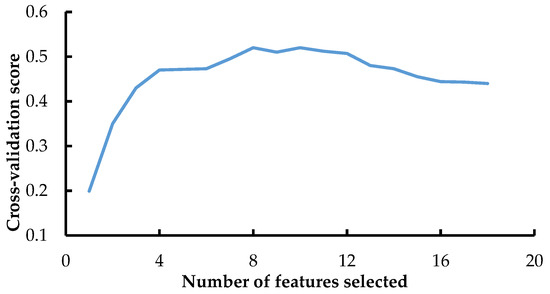
Figure 4.
Results of feature screening by RFE with 5-fold CV.
The matrix permeability and perforation thickness were two most important geological properties of the tight formation. Moreover, the volumes of slurry fluid and proppant injected per well is two of the most important fracturing treatment parameters in predicting the well AOFP.
4.2. Hyperparameter Tuning for ML Models
ML models involve many hyperparameters, but only a few crucial parameters are necessary to be tuned to achieve optimal performance. In this study, a grid search technique with five-fold cross-validation was employed to find the optimal tuning hyperparameters based on the root mean square error (RMSE) value for each ML method. The hyperparameters used in developing the three predictive ML models were presented in Table 3.
Table 3.
The hyperparameters for tuning the ML models.
4.3. Performance of Each ML Model
Table 4 presents the results of the three statistical indicators of the model prediction in both the training and test datasets, which include MAE (Mean Absolute Error), MSE (Mean Squared Error), and coefficient of determination (R2). It was observed that the GBDT model outperformed the other two methods on both the training and test sets. As a result, the GBDT algorithm was selected to construct the prediction model. Figure 5 illustrates the prediction fitting results of the GBDT model. Further interpretability analysis will be conducted on the GBDT model in the subsequent subsection.
Table 4.
Statistical results of evaluation indicators for the three models.
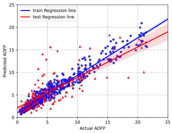
Figure 5.
Comparison of predicted and actual AOFP for the GBDT model.
4.4. GBDT Model Interpretations
4.4.1. Global Interpretation with SHAP
Figure 6a shows global feature importance according to the average of the absolute SHAP values for each input variable. A larger mean SHAP value corresponds to a greater influence on the well AOFP. It can be clearly observed from Figure 6a that variable FP (flowing bottom-hole pressure) is the most significant variable, followed by variables PERM (matrix permeability) and SFV (slurry fluid volume).
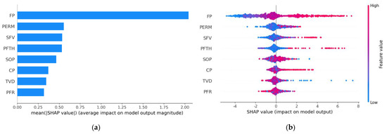
Figure 6.
Global interpretation of the GBDT model: (a) SHAP global feature importance plot; (b) SHAP summary plot for the well AOFP.
Figure 6b shows the SHAP summary plot, where each point is a Shapely value for each feature and individual data point. The vertical color bar demonstrates low to high transition from blue to red. The plot allows us to analyze the feature’s importance together with its magnitude and effect direction. Figure 6b shows that the variable FP has a positive impact on the well AOFP. As the value of FP increases, the SHAP value increases, increasing well productivity. By contrast, an increase in TVD (well true vertical depth) will decrease the value of well AOFP.
Figure 7 provides a more detailed understanding of the impact of input variables on the AOFP and the correlation between them. The analysis of SHAP values reveals that perforation thickness (PFTH) and slurry fluid volume (SFV) has a positive correlation with the AOFP, as indicated by the increasing SHAP values with increasing SFV as shown in Figure 7a. Additionally, the plot suggests that for thicker gas zones, it is necessary to increase the usage of slurry fluid. The analysis of SHAP values for matrix permeability demonstrates that for formation with matrix permeability less than 2 mD, increasing the amount of proppant during hydraulic fracturing is essential as demonstrated in Figure 7b. These insights into the impact of input variables on the well AOFP provide valuable guidance for optimizing hydraulic fracturing design and maximizing gas recovery in tight gas reservoirs.
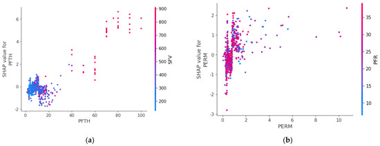
Figure 7.
Feature dependence plots: (a) Perforation thickness (PFTH) vs. Slurry fluid volume (SFV); (b) Matrix permeability (PERM)vs. Proppant fluid ratio (PFR).
4.4.2. Local Interpretation with SHAP and LIME
To illustrate the interpretability of the GBDT model using SHAP and LIME methods, one fractured vertical well from the test dataset, Sudong 59-11E, was provided. The arrows in Figure 8a show the influence of each factor on the prediction, with blue and red indicating whether the factor reduced or increased the prediction, respectively. The length of the bar indicates the extent of the related increases and declines, and the base value is the average of the predictions of the database, which is 5.891 (104 m3/d). The figure shows that the value of perforation thickness (PFTH) in this sample would increase the predicted productivity by 4.807 (104 m3/d) relative to the baseline value, while the value of casing pressure in this sample would decrease the predicted value by 0.8458 (104 m3/d) relative to the baseline value. By combining the base value and the SHAP values for all the features, the final prediction of 16.93 (104 m3/d) was obtained, which is very close to the real value of 15.51 (104 m3/d). These results demonstrate the potential of SHAP in providing detailed insights into the effects of different features on the well productivity and quantitatively analyzing their contributions.
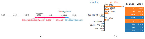
Figure 8.
Local interpretation of well Sudong 59-11E: (a) with SHAP; (b) with LIME.
In Figure 8b, the LIME local interpretation technique is employed to summarize the factors contributing to the AOFP prediction of well Sudong 59-11E. The orange-colored factors indicate a positive contribution to productivity prediction, while the blue-colored factors indicate a negative contribution. The table on the right of the figure provides a rank of the contribution of each feature to the prediction along with the feature’s actual value. The results show that bottom-hole pressure, slurry fluid volume, perforation thickness, and casing pressure all positively contribute to the productivity prediction, which is consistent with the SHAP local interpretation. On the other hand, matrix permeability, true vertical depth, proppant fluid ratio, and tubing pressure all have a negative impact on the AOFP prediction. The use of LIME and SHAP together provides a more detailed and comprehensive understanding of the model’s decision-making process, which can aid in improving the model’s performance and building trust among petroleum engineers.
4.5. Reflections and Implications
The case study provided valuable insights into the use of machine learning techniques in the oil and gas industry. First, the interpretability of predictive models is crucial for model transparency and accountability in the petroleum industry. Furthermore, the utilization of multiple interpretability techniques, such as SHAP and LIME, can provide complementary insights and improve the overall reliability of the model. Finally, the importance of domain knowledge and expert input in the feature engineering process cannot be overstated, as this can significantly enhance the model’s accuracy and interpretability. These findings have important implications for the development and deployment of machine learning models in the petroleum industry and can inform best practices for future projects.
The study provides practical insights for petroleum engineers involved in the field development and optimization of tight gas production. By using ML models and interpreting the feature importance, the key reservoir parameters and completion strategies can be identified that impact well productivity. This can help them make more informed decisions about the well completion and stimulation practices, leading to more efficient and effective tight gas field development.
The study has the potential to contribute to the sustainable development of tight gas reservoirs. By improving the understanding of the factors that influence well productivity, The development and production of these resources can be optimized while minimizing their environmental impact. This can help to ensure the long-term viability of tight gas reservoirs as a source of energy for society.
5. Conclusions
This study provides a comprehensive methodology for evaluating the well productivity prediction models for tight gas reservoirs using an interpretable machine learning approach. The complex non-linear relationship between the input features and the absolute open flow potential (AOFP) was investigated by interpretable ML modeling. The performance of various ML models is assessed based on the MSE, MAE, and R2. The GBDT model, which exhibited the best prediction efficacy among all trained models, was selected for further analysis.
The SHAP-based model interpretability technique was employed to provide a clear interpretation of the predicted results in terms of the relative importance of different input features. Based on the SHAP values, it was identified that bottom-hole pressure, matrix permeability, and slurry fluid volume have the most significant impact on the well productivity. This evaluation of the relative importance of different features and their influence on well productivity is expected to help petroleum engineers optimize field operations.
In addition, the assessment of feature contribution to the productivity prediction of a single fractured well by SHAP and LIME provided a detailed understanding of the model’s decision-making process. The local interpretation techniques were valuable for identifying potential errors, biases, or areas for improvement in the model, which is essential for building trust among engineers, and will potentially facilitate the development of better physics-based predictive models for undrilled wells.
Overall, this study highlights the potential of the ML techniques in predicting well productivity in tight gas reservoirs. The integration of the ML with the interpretation methods can provide a comprehensive understanding of the model’s performance and decision-making process, leading to the effective development of the tight gas field.
Author Contributions
Conceptualization, X.M. and J.Z.; methodology, X.M.; validation, M.H. and Z.L.; formal analysis, X.M.; investigation, X.M. and J.Z.; data curation, X.M.; writing—original draft preparation, X.M.; writing—review and editing, X.M. and J.Z.; visualization, M.H. and Z.L.; funding acquisition, X.M. All authors have read and agreed to the published version of the manuscript.
Funding
This research was funded by the National Natural Science Foundation of China (Grant Nos. 51974253, 51934005, 52004219), the Natural Science Basic Research Program of Shaanxi (Grant Nos. 2017JM5109 and 2020JQ-781), the Scientific Research Program Funded by Education Department of Shaanxi Province (Grant Nos. 18JS085 and 20JS117), and the Graduate Student Innovation and Practical Ability Training Program of Xi’an Shiyou University (Grant No. YCS21211021).
Data Availability Statement
Data is unavailable due to commercial restraints.
Conflicts of Interest
The authors declare no conflict of interest.
References
- Li, G.; Lei, Z.; Dong, W.; Wang, H.; Zheng, X.; Tan, J. Progress, challenges and prospects of unconventional oil and gas development of CNPC. China Pet. Explor. 2022, 27, 1–11. [Google Scholar]
- Zou, C.; Zhu, R.; Dong, D.; Wu, S. Scientific and technological progress, development strategy and policy suggestion regarding shale oil and gas. Acta Pet. Sin. 2022, 43, 1675–1686. [Google Scholar]
- Jia, A.; Wei, Y.; Guo, Z.; Wang, G.; Meng, D.; Huang, S. Development status and prospect of tight sandstone gas in China. Nat. Gas Ind. B 2022, 9, 467–476. [Google Scholar] [CrossRef]
- Li, G.; Zhu, R. Progress, challenges and key issues of unconventional oil and gas development of CNPC. China Pet. Explor. 2020, 25, 1–13. [Google Scholar]
- Zou, C.; Pan, S.; Jing, Z.; Gao, J.; Yang, Z.; Wu, S.; Zhao, Q. Shale oil and gas revolution and its impact. Acta Petrolei Sinica 2020, 41, 1–12. [Google Scholar]
- Ma, X.; Zhou, D.; Cai, W.; Li, X.; He, M. An interpretable machine learning approach to prediction horizontal well productivity. J. SW Pet. Univ. 2022, 44, 81–90. [Google Scholar]
- Xu, S.; Feng, Q.; Wang, S.; Javadpour, F.; Li, Y. Optimization of multistage fractured horizontal well in tight oil based on embedded discrete fracture model. Comput. Chem. Eng. 2018, 117, 291–308. [Google Scholar] [CrossRef]
- Moinfar, A.; Narr, W.; Hui, M.; Mallison, B.T.; Lee, S.H. Comparison of Discrete-Fracture and Dual-Permeability Models for Multiphase Flow in Naturally Fractured Reservoirs; SPE Reservoir Simulation Symposium: The Woodlands, TX, USA, 2011. [Google Scholar] [CrossRef]
- Moinfar, A.; Varavei, A.; Sepehrnoori, K. Development of an efficient embedded discrete fracture model for 3D compositional reservoir simulation in fractured reservoirs. SPE J. 2014, 19, 289–303. [Google Scholar] [CrossRef]
- Yang, Z.; Chen, Q.; Li, X.; Fang, B.; Liu, Z. A new method for calculating the productivity of the staged multi-bunch fractured horizontal well in tight gas reservoirs. Pet. Geol. Oilfield Dev. Daqing 2019, 38, 147–154. [Google Scholar] [CrossRef]
- Chen, C.; He, W.; Zhou, H.; Zhu, M. A comparative study among machine learning and numerical models for simulating groundwater dynamics in the Heihe River Basin, northwestern China. Sci. Rep. 2020, 10, 3904. [Google Scholar] [CrossRef]
- Sun, F.; Hang, S.; Chen, L.; Li, X. Coupled model for seepage and wellbore flow of fractured horizontal wells in low-permeability gas reservoirs. J. SW Pet. Inst. 2005, 27, 32–37. [Google Scholar]
- Clarkson, C.R.; Qanbari, F. A semianalytical forecasting method for unconventional gas and light oil wells: A hybrid approach for addressing the limitations of existing empirical and analytical Methods. SPE Res. Eval. Eng. 2015, 18, 94–110. [Google Scholar] [CrossRef]
- Li, G.; Guo, B.; Li, J.; Wang, M. A mathematical model for predicting long-term productivity of modern multifractured shale-gas/oil wells. SPE Drill Compl. 2019, 34, 114–127. [Google Scholar] [CrossRef]
- Jiang, J.; Rami, M.Y. Hybrid coupled discrete-fracture/matrix and multicontinuum models for unconventional reservoir simulation. SPE J. 2016, 21, 1009–1027. [Google Scholar] [CrossRef]
- Zhang, M.; Ayala, L.F. The dual-reciprocity boundary element method solution for gas recovery from unconventional reservoirs with discrete fracture networks. SPE J. 2020, 25, 2898–2914. [Google Scholar] [CrossRef]
- Wantawin, M.; Yu, W.; Sepehrnoori, K. An iterative workflow for history matching by use of design of experiment, response-surface methodology, and Markov chain Monte Carlo algorithm applied to tight oil reservoirs. SPE Reserv. Eval. Eng. 2017, 20, 613–626. [Google Scholar] [CrossRef]
- Xue, L.; Liu, Y.; Xiong, Y.; Liu, Y.; Cui, X.; Lei, G. A data-driven shale gas production forecasting method based on the multi-objective random forest regression. J. Pet. Sci. Eng. 2021, 196, 107801. [Google Scholar] [CrossRef]
- Dong, Y.; Qiu, L.; Lu, C.; Song, L.; Ding, Z.; Yu, Y.; Chen, G. A data-driven model for predicting initial productivity of offshore directional well based on the physical constrained eXtreme gradient boosting (XGBoost) trees. J. Pet. Sci. Eng. 2022, 211, 110176. [Google Scholar] [CrossRef]
- Wang, S.; Chen, S. Insights to fracture stimulation design in unconventional reservoirs based on machine learning modeling. J. Pet. Sci. Eng. 2019, 174, 682–695. [Google Scholar] [CrossRef]
- Wang, L.; Yao, Y.; Wang, K.; Adenutsi, C.D.; Zhao, G.; Lai, F. Hybrid application of unsupervised and supervised learning in forecasting absolute open flow potential for shale gas reservoirs. Energy 2022, 243, 122747. [Google Scholar] [CrossRef]
- Morozov, A.D.; Popkov, D.O.; Duplyakov, V.M.; Mutalova, R.F.; Osiptsov, A.A.; Vainshtein, A.L.; Burnaev, E.V.; Shel, E.V.; Paderin, G.V. Data-driven model for hydraulic fracturing design optimization: Focus on building digital database and production forecast. J. Pet. Sci. Eng. 2020, 194, 107504. [Google Scholar] [CrossRef]
- Porras, L.; Hawkes, C.; Arshad, I. Evaluation and optimization of completion design using machine learning in an unconventional light oil play. In Proceedings of the 8th Unconventional Resources Technology Conference, Virtual, 20–22 July 2020. [Google Scholar] [CrossRef]
- Rahmanifard, H.; Alimohamadi, H.; Gates, I. Well Performance Prediction in Montney Formation Using Machine Learning Approaches. In Proceedings of the SPE/AAPG/SEG Unconventional Resources Technology Conference, Virtual, 20–22 July 2020. [Google Scholar] [CrossRef]
- Luo, G.; Tian, Y.; Bychina, M.; Ehlig-Economides, C. Production-strategy insights using machine learning: Application for Bakken Shale. SPE Res. Eval. Eng. 2019, 22, 800–816. [Google Scholar] [CrossRef]
- Molnar, C. Interpretable Machine Learning. Available online: https://christophm.github.io/interpretable-ml-book/ (accessed on 11 February 2022).
- Murdoch, W.J.; Singh, C.; Kumbier, K.; Abbasi-Asl, R.; Yu, B. Interpretable machine learning: Definitions, methods, and applications. Proc. Natl. Acad. Sci. USA 2019, 116, 22071–22080. [Google Scholar] [CrossRef] [PubMed]
- Wang, M.; Tang, H.; Zhao, F.; Liu, S.; Yang, Y.; Zhang, L.; Liao, J.; Lu, H. Controlling factor analysis and prediction of the quality of tight sandstone reservoirs: A case study of the He8 Member in the eastern Sulige Gas Field, Ordos Basin, China. J. Nat. Gas Sci. Eng. 2017, 46, 680–698. [Google Scholar] [CrossRef]
- Wang, J.; Zhang, C.; Li, J. Tight sandstone gas reservoirs in the Sulige gas field: Development understandings and stable-production proposals. Nat. Gas Ind. 2021, 41, 100–110. [Google Scholar]
- Ma, X.; Fan, Y. Productivity prediction model for vertical fractured well based on machine learning. Math. Pract. Theory 2021, 51, 186–196. [Google Scholar]
- Breiman, L. Random forests. Mach. Learn. 2001, 45, 5–32. [Google Scholar] [CrossRef]
- Pedregosa, F.; Weiss, R.; Brucher, M. Scikit-learn: Machine learning in Python. J. Mach. Learn. Res. 2011, 12, 2825–2830. [Google Scholar]
- Friedman, J.H. Greedy function approximation: A gradient boosting machine. Ann. Stat. 2001, 29, 1189–1232. [Google Scholar] [CrossRef]
- Scholkopf, B.; Smola, A.J. Learning with Kernels: Support Vector Machines, Regularization, Optimization, and Beyond; MIT Press: Cambridge, MA, USA, 2002. [Google Scholar]
- Vapnik, V.N. The Nature of Statistical Learning Theory; Springer: New York, NY, USA, 2013. [Google Scholar]
- Chen, Z.; Xiao, F.; Guo, F.; Yan, J. Interpretable machine learning for building energy management: A state-of-the-art review. Adv. Appl. Energy 2023, 9, 100123. [Google Scholar] [CrossRef]
- Kamath, U.; Liu, J. Explainable Artificial Intelligence: An Introduction to Interpretable Machine Learning; Springer International Publishing: Cham, Switzerland, 2021. [Google Scholar] [CrossRef]
- Lundberg, S.M.; Lee, S.I. A unified approach to interpreting model predictions. In Proceedings of the 31st International Conference on Neural Information Processing Systems, Long Beach, CA, USA, 4–9 December 2017; pp. 4768–4777. [Google Scholar]
- Ribeiro, M.; Singh, S.; Guestrin, C. “Why Should I Trust You?”: Explaining the predictions of any classifier. In Proceedings of the 22nd ACM SIGKDD International Conference on Knowledge Discovery and Data Mining, San Francisco, CA, USA, 13–17 August 2016; pp. 1135–1144. [Google Scholar]
- Feng, X.; Zhong, F.; Wang, H.; Xiong, Y.; Zeng, L. Modified single point method to evaluate productivity of gas wells with big production for Feixianguan Group gas reservoies in northeast Sichuan. Nat. Gas Ind. 2005, 25, 107–109. [Google Scholar]


Disclaimer/Publisher’s Note: The statements, opinions and data contained in all publications are solely those of the individual author(s) and contributor(s) and not of MDPI and/or the editor(s). MDPI and/or the editor(s) disclaim responsibility for any injury to people or property resulting from any ideas, methods, instructions or products referred to in the content. |
© 2023 by the authors. Licensee MDPI, Basel, Switzerland. This article is an open access article distributed under the terms and conditions of the Creative Commons Attribution (CC BY) license (https://creativecommons.org/licenses/by/4.0/).