
Energy Performance Comparison of a Chiller Plant Using the Conventional Staging and the Co-Design Approach in the Early Design Phase of Hotel Buildings
 ,
,
Abstract
:1. Introduction
2. Materials and Methods
2.1. Methodology
- Calculation of the cooling load demand of the building.
- Implementation of accurate energy models of the HVAC systems for simulation purposes.
- Implementation of chiller plant sequencing algorithm and energy performance evaluation.
2.2. Cooling Load Demand of Building
- Consideration in the simulation of activity levels in public areas and the activity patterns of hotels near the case study, which have in common the type of hotel, total capacity, and type of tourism.
- Consideration of the variation in the occupancy levels in each thermal zone with the aid of the historical occupancy levels in similar hotels.
- Establishment of energy efficiency measures in the thermal zones related to the rooms’ areas according to the suggestions of Yang et al. [6].
- Establishment of the concept of a partially loaded room for thermal zones belonging to the rooms. This measure included comfort conditions in unoccupied rooms, considering a set point of 25 °C, which ensured high indoor air quality levels in tropical-climate hotels.
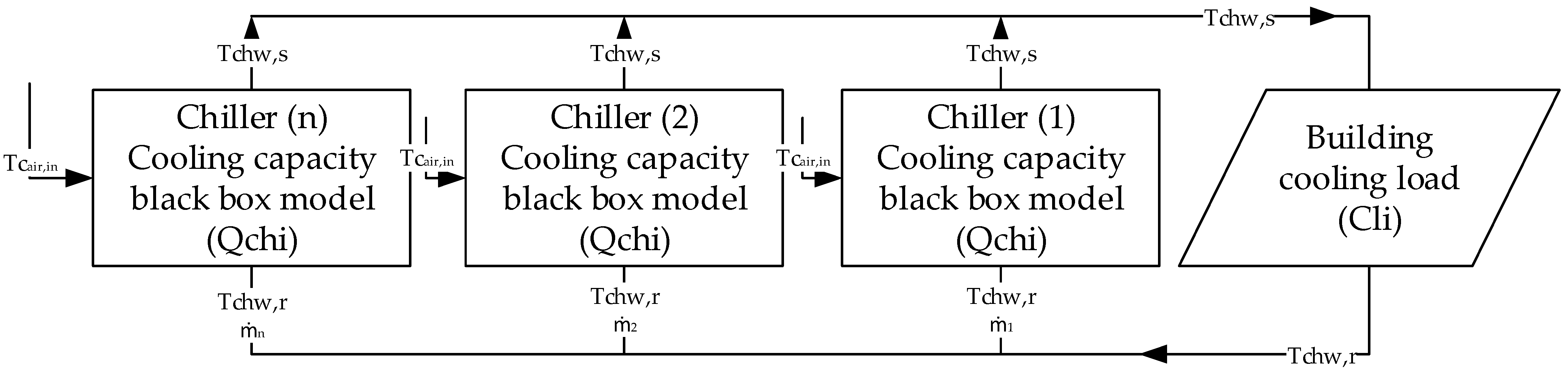
2.3. Implementation of Accurate Simulation Models of Air-Cooled Chiller Unit
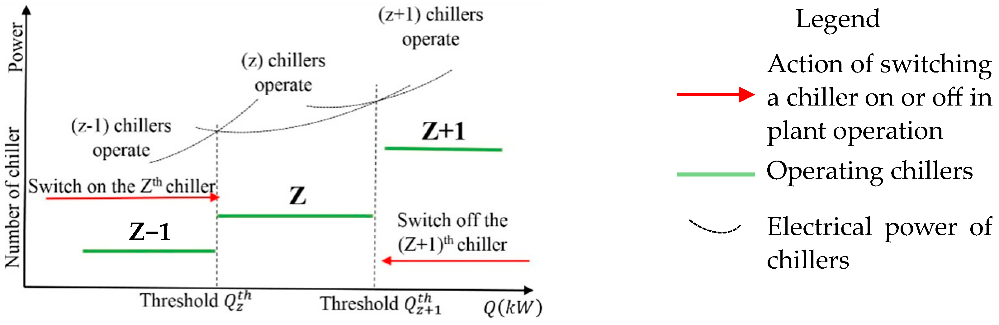
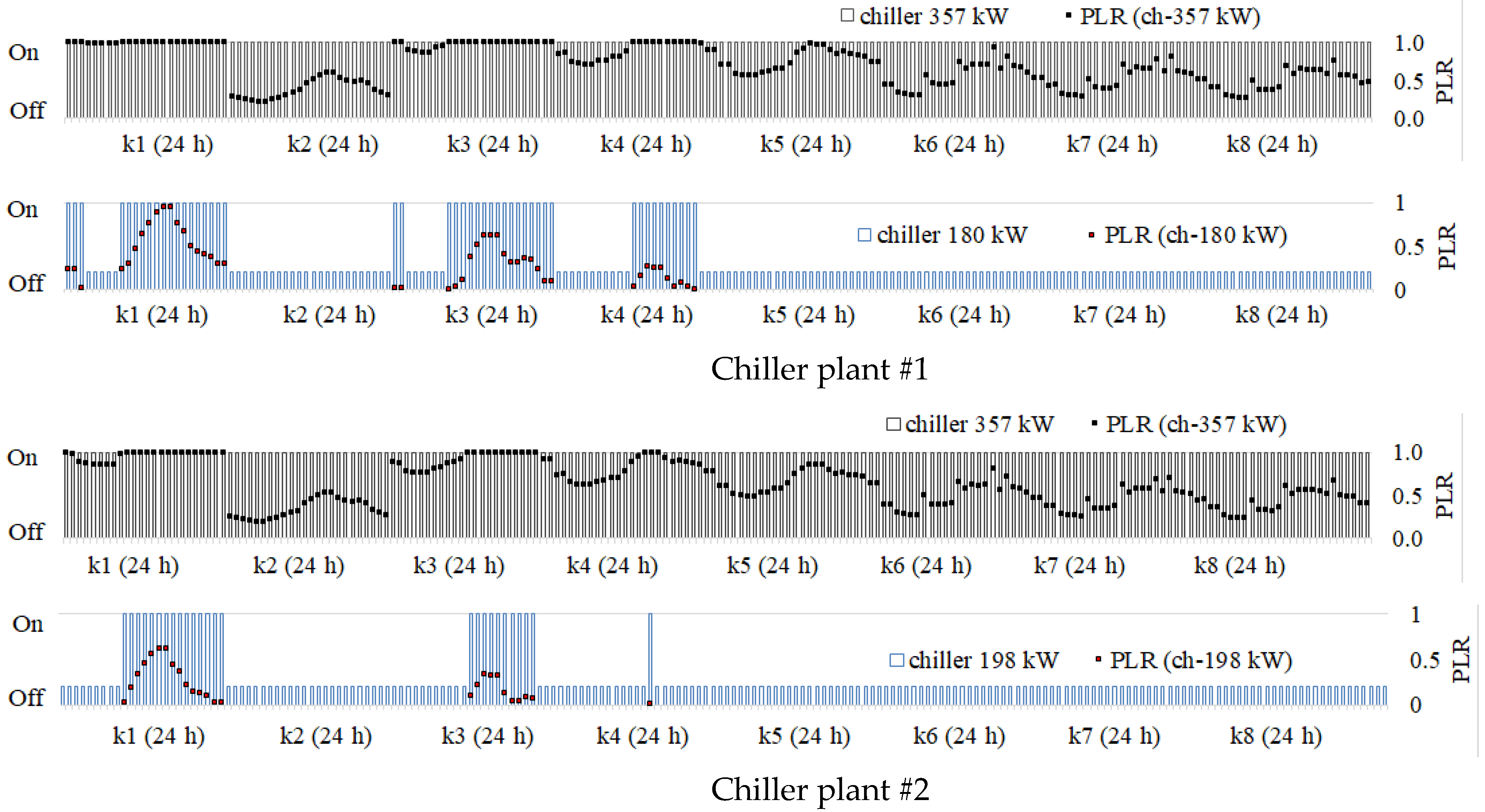
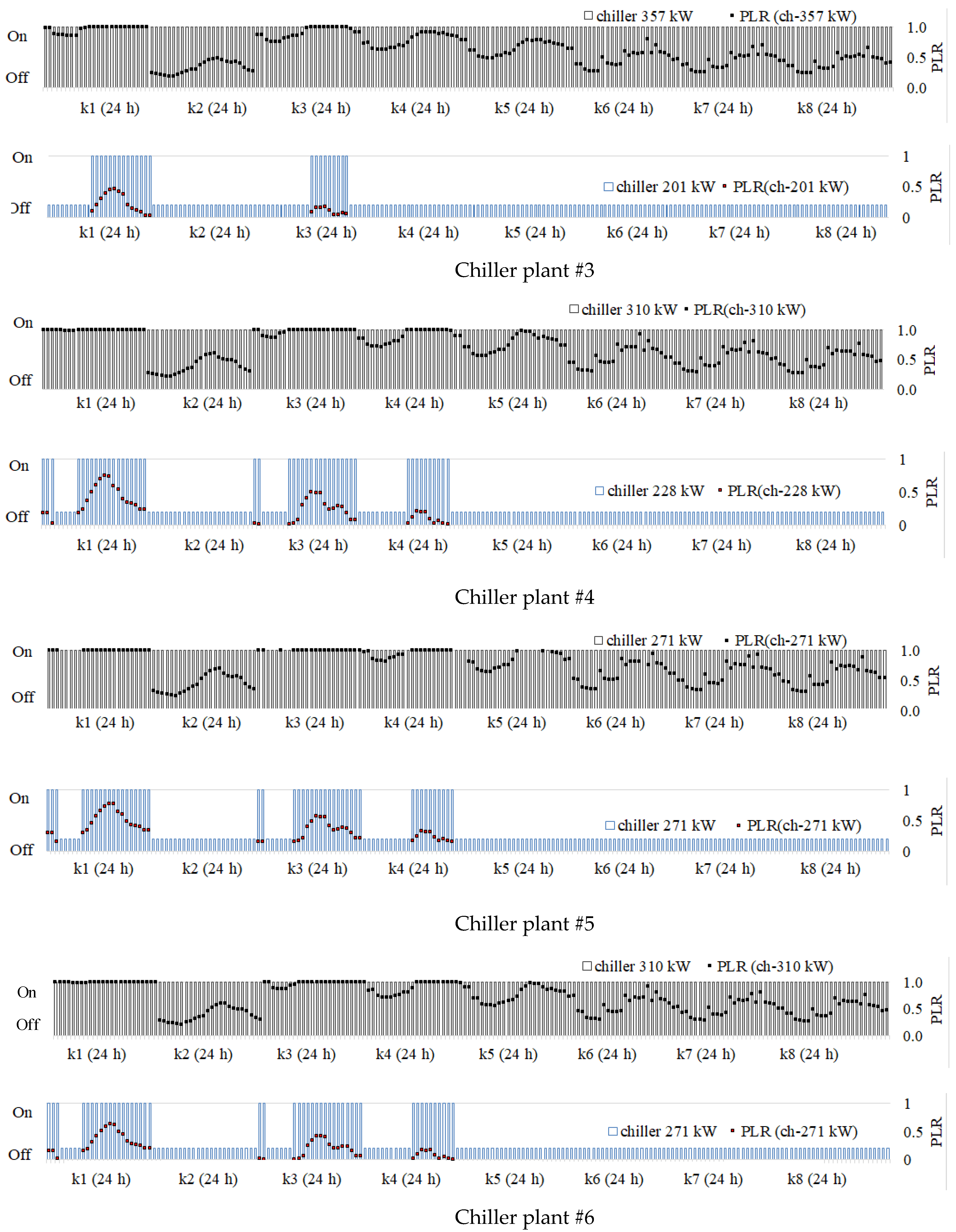
2.3.1. Approach Using the Traditional Principle of Chiller On/Off Staging
- Step 1: If cooling load CLi ≤ Qch1, then chiller 1 satisfied the system load (with Qch1 > Qch2);
- Step 2: If Cli > Qch1, then chiller 1 provided the full cooling load and the remaining thermal demand was provided by chiller 2;
- Step 3: If Cli ≥ Qch1 + Qch2 +…Qchn+, then chillers Ch1, Ch2,…, Chn were turned on (in which Qch1 > Qch2> … > Qchn).
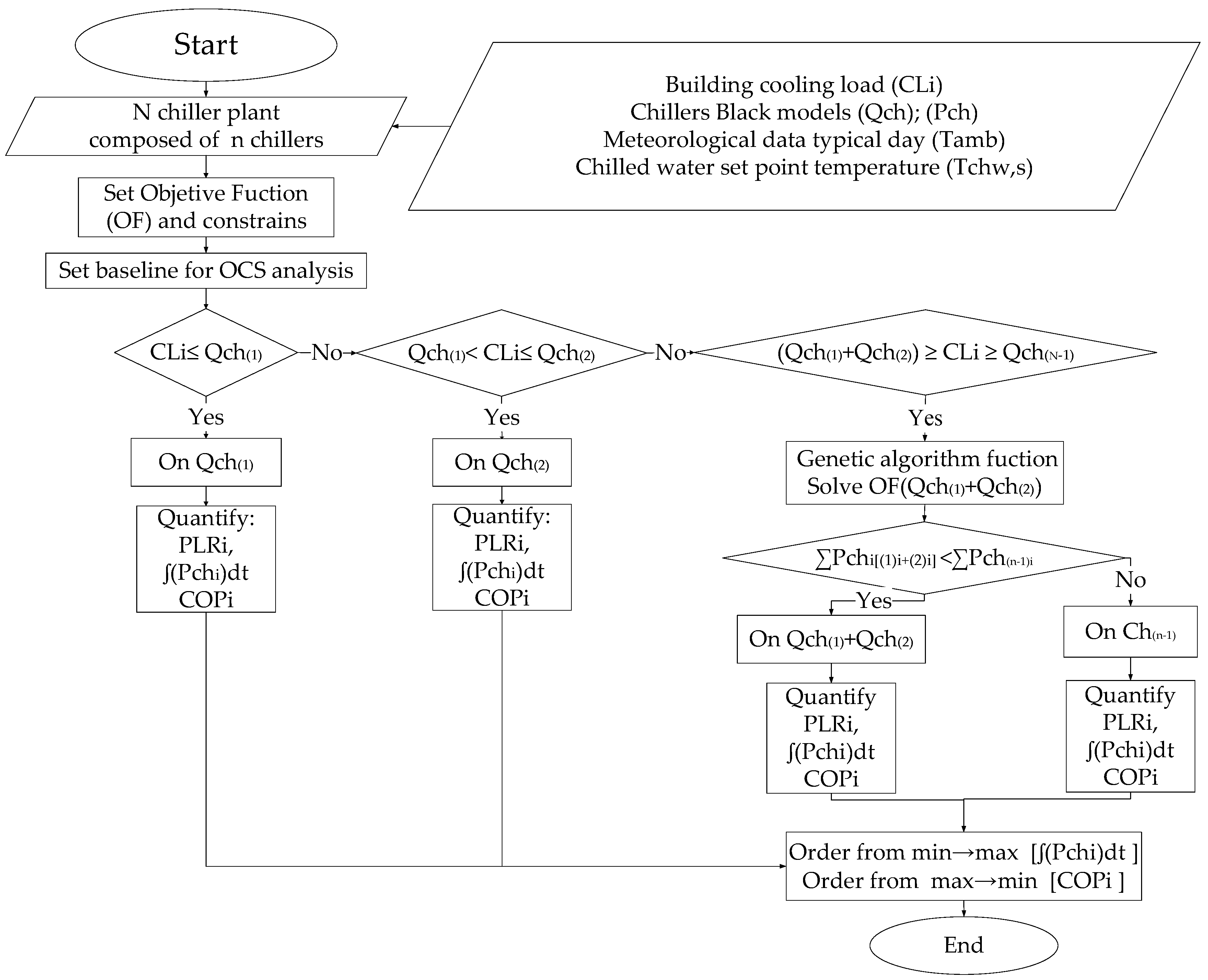
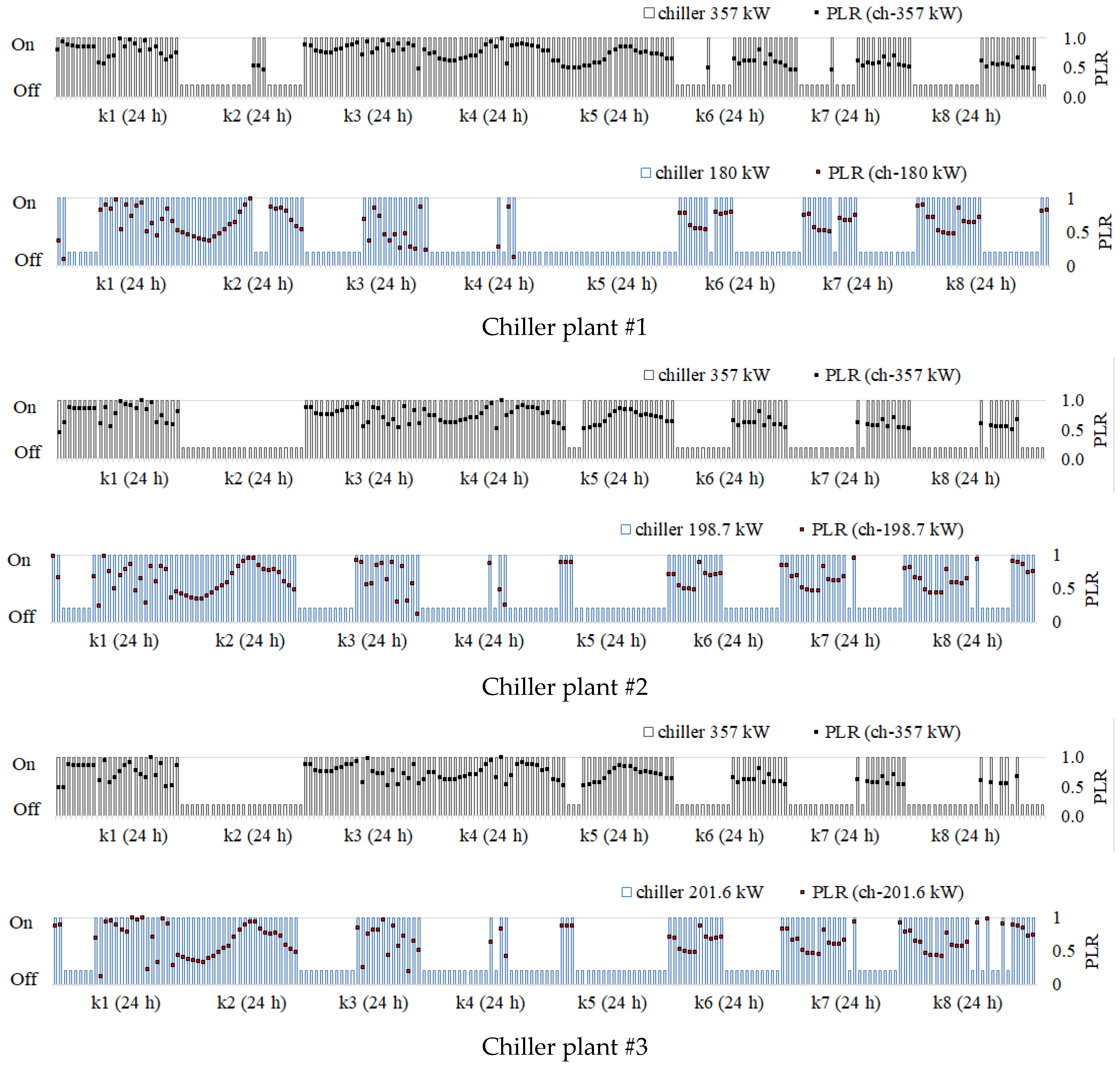
2.3.2. Optimal Chiller Loading and Optimal Chiller Sequence Staging Approach: Co-Design of Chiller Plant Approach
- Step 1: If CLi ≤ Qch1,i, then chiller 1 satisfied the system load;
- Step 2: If Qch1,i < CLi ≤ Qch2,i, then chiller 2 met system load;
- Step 3: If (Qch1,i + Qch2,i) ≤ CLi ≤ Qchn−1,i, the OF of chillers 1 and 2 was optimized and derived from the optimal load problem, and the results were quantified. The results were compared with the electrical power consumption of the chiller (n − 1). If (Pch1,i + Pch2,i) < Pchn−1, chillers 1 and 2 were turned on. If not, chiller n − 1 turned on;
- Step 4: If CLi≥ Qch1,i + Qch2,i +… Qchn,i, then chillers 1, 2,…, n were turned on. OF was optimized for chillers 1,2,…, n.
3. Case Study
- (1)
- The concept of a “partially loaded” room (unoccupied rooms which were kept at 26 °C by an air conditioner) was applied [32].
- (2)
- Different occupancy rates between 10%, 50%, 75%, and 100% for the hotel in the rooms and public areas were considered.
- (3)
- The load diversity through occupancy strategies was eliminated using the lowest-thermal-demand rooms for occupancy rates of 75% and 50%.
4. Results and Discussion
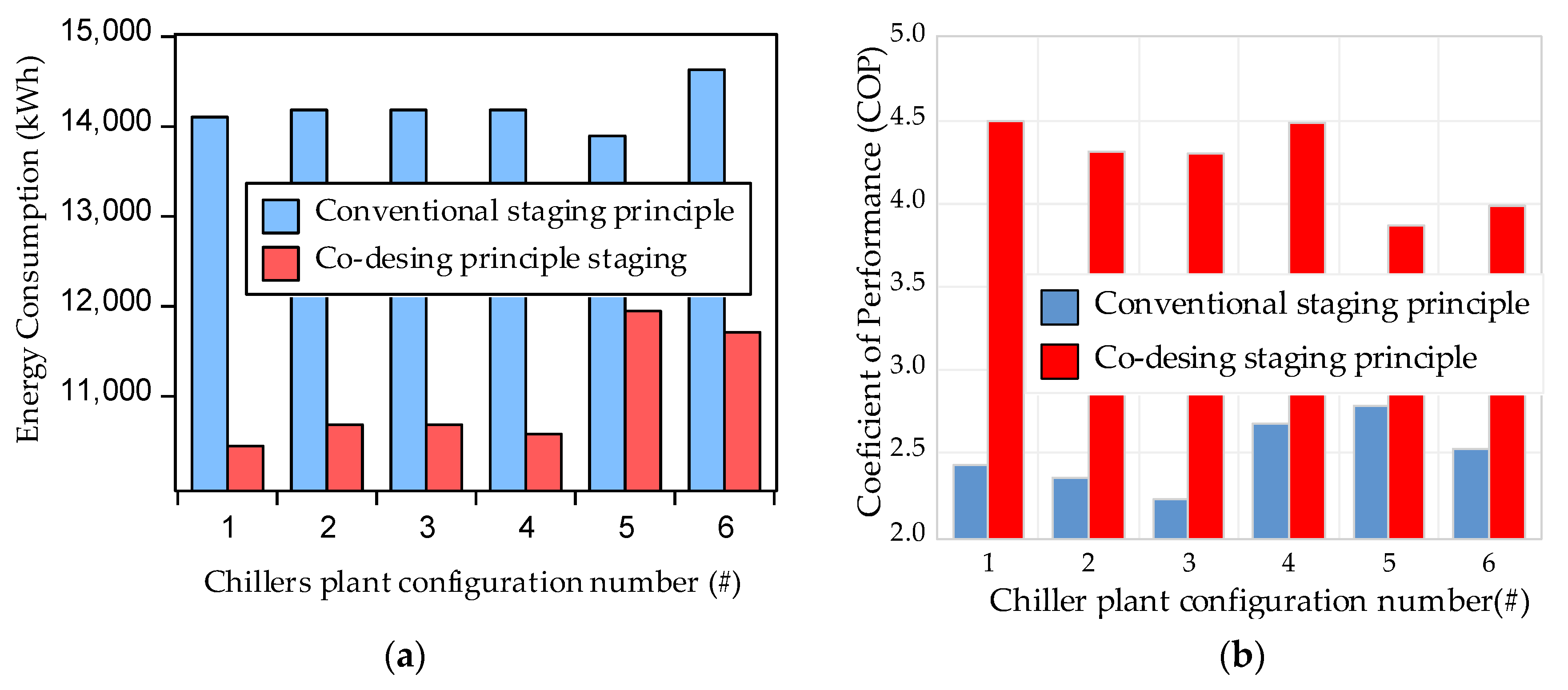
- The application of the traditional load-based sequencing methodology suggested the adoption of chiller plant configuration #5, which showed an energy consumption of 13,882.52 kWh and an average COP of 2.78.
- The implementation of the proposed optimization approaches suggested that the best option would be the adoption of chiller plant configuration #1 (asymmetric configuration, chiller cooling capacity distribution of 33/67%, safety factor of 10.2%), which showed an energy consumption of 10,446.25 kWh and an average COP of 4.44.
5. Conclusions
Author Contributions
Funding
Data Availability Statement
Conflicts of Interest
Nomenclatures
| Annex 1: Nomenclature | |
| a0, a1, a2 | Correlation coefficients of the black box model of electrical power |
| BLR | Building load ratio |
| CI | Specific consumption index |
| CLi | Building cooling load for each interval of time i (kW) |
| Comb | Combinations of chiller plant |
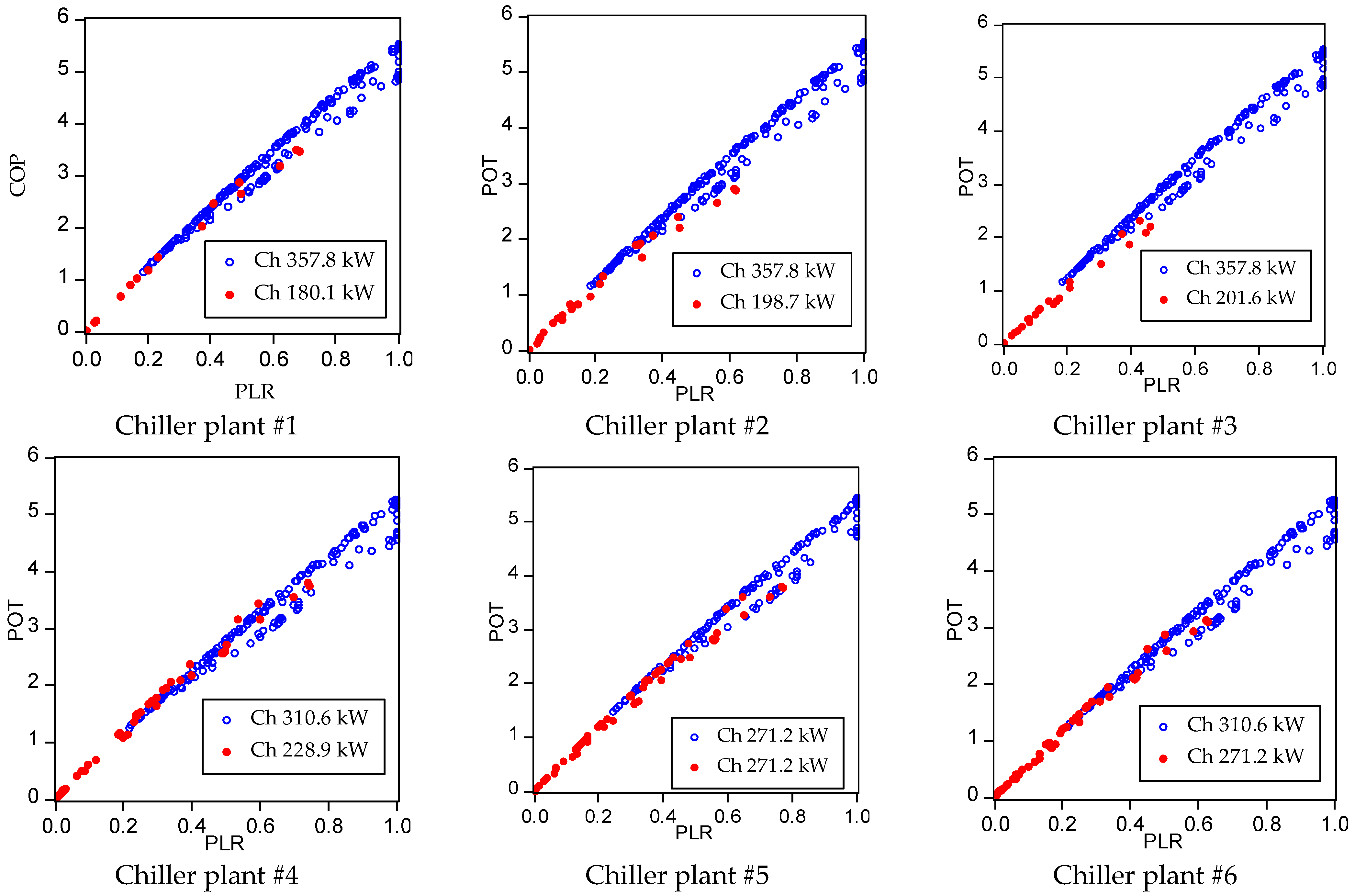
| COP | Coefficient of performance |
| cp | Specific heat at constant pressure of water at 7 °C (kJ/(Kg·K)) |
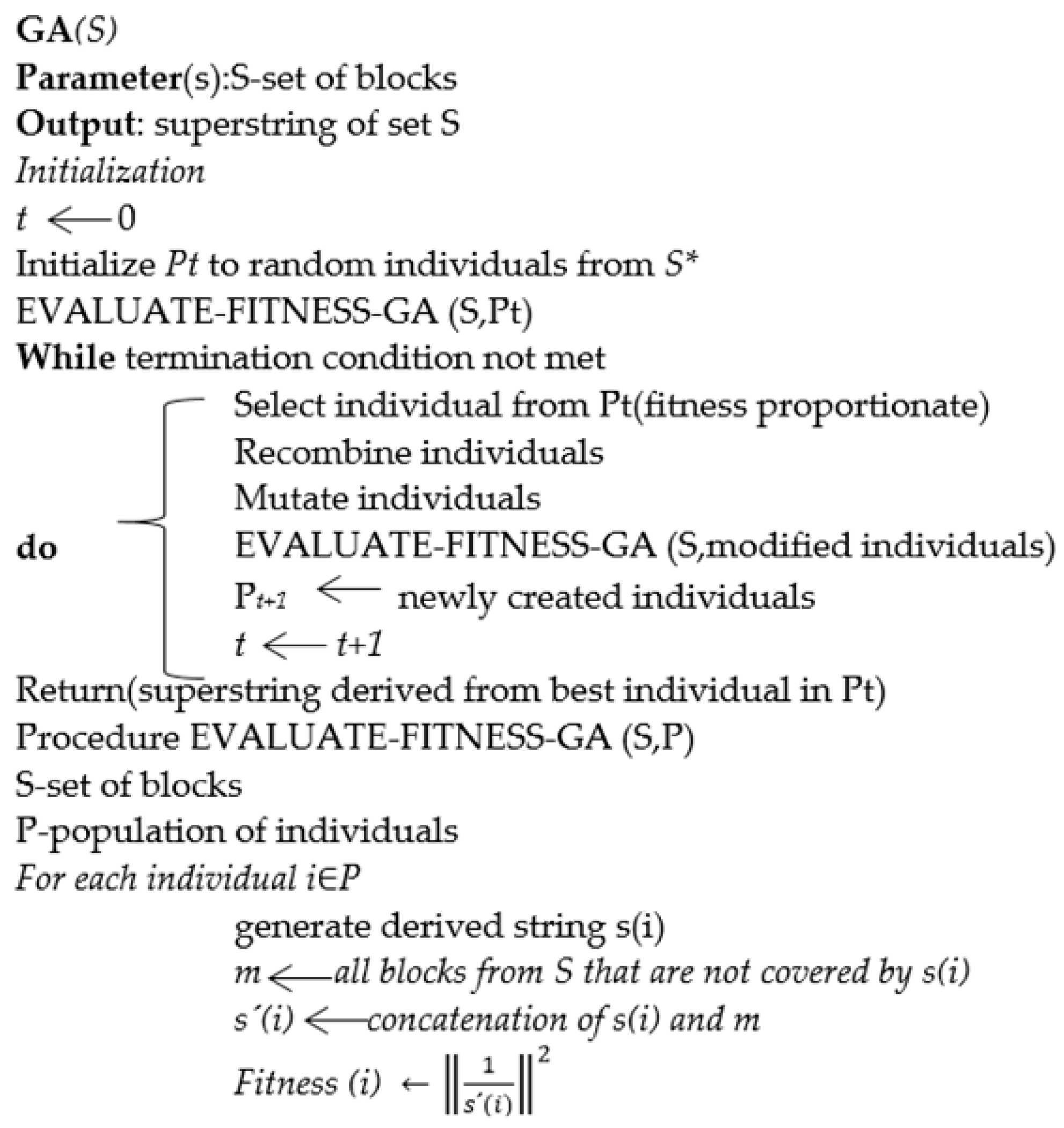
| GA | Genetic algorithm |
| Hdo | Occupied room indicator |
| ki | Simulation scenario |
| ṁ | Chilled-water mass flow (Kg/s) |
| nch | Total of chiller selected in each chiller plant |
| OCL | Optimal chiller loading |
| OCS | Optimal chiller sequencing |
| Pch | Power consumption of chiller (kW) |
| PLR | Partial load ratio |
| Qch | Cooling load for the chiller (kW) |
| Qcl | Total cooling load (kW) |
| Qchstd | Cooling capacity of the chiller at standard conditions according to manufacturer (kW) |
| Qcho | Cooling capacity of the reference chiller (kW) |
| Sj off | Stage off threshold |
| Sj on | Stage on threshold |
| Tc air,in | Condenser air inlet temperature (°C) |
| Tc hw,s | Chiller water supply temperature (°C) |
| Tc hw,r | Chiller water return temperature (°C) |
| x0, x1, x2 | Correlation coefficients of the black box model of nominal cooling capacity |
| Subscripts | |
| ch | Chiller water |
| i | ith |
| max | Maximum |
| min | Minimum |
| c | Condenser |
| in | Inlet |
| s | Supply |
| r | Return |
References
- Fang, X.; Jin, X.; Du, Z.; Wang, Y.; Shi, W. Evaluation of the design of chilled water system based on the optimal operation performance of equipments. Appl. Therm. Eng. 2017, 113, 435–448. [Google Scholar] [CrossRef]
- ASHRAE. ASHRAE Fundamentals Handbook; ASHRAE: Peachtree Corners, GA, USA, 2017; ISBN 10: 1939200598. [Google Scholar]
- Díaz Torres, Y.; Álvarez Guerra Plasencia, A.; Viego Felipe, P.; Crespo Sanchez, G.; Diaz Gonzalez, M. Chiller plant design. Review of the aspects that involve its efficient design. Ing. Energética 2020, 41, e1711. [Google Scholar]
- Taylor, S. Fundamentals of Design and Control of Central Chilled-Water Plans (I-P); Atlanta ASHRAE: Peachtree Corners, GA, USA, 2017; ISBN 978-1-939200-67-9. [Google Scholar]
- Cheng, Q.; Wang, S.; Yan, C. Sequential Monte Carlo simulation for robust optimal design of cooling water system with quantified uncertainty and reliability. Energy 2016, 118, 489–501. [Google Scholar] [CrossRef]
- Yan, C.; Cheng, Q.; Cai, H. Life-Cycle optimization of a chiller plant with quantified analysis of uncertainty and reliability in commercial buildings. Appl. Sci. 2019, 9, 1548. [Google Scholar] [CrossRef]
- Huang, P.; Huang, G.; Augenbroe, G.; Li, S. Optimal configuration of multiple-chiller plants under cooling load uncertainty for different climate effects and building types. Energy Build. 2018, 158, 684–697. [Google Scholar] [CrossRef]
- Li, H.; Wang, S.; Xiao, F. Probabilistic optimal design and on-site adaptive commissioning of building air-conditioning systems concerning uncertainties. Energy Procedia 2019, 158, 2725–2730. [Google Scholar] [CrossRef]
- Sun, Y.; Wang, S.; Huang, G. Chiller sequencing control with enhanced robustness for energy efficient operation. Energy Build. 2009, 41, 1246–1255. [Google Scholar] [CrossRef]
- Gang, W.; Wang, S.; Xiao, F.; Gao, D.-c. Robust optimal design cooling systems considering cooling load uncertainty and equipment reliability. Appl. Energy 2015, 159, 265–275. [Google Scholar] [CrossRef]
- Gang, W.; Wang, S.; Yan, C.; Xiao, F. Robust optimal design of building cooling systems concerning uncertainties using mini-max regret theory. Sci. Technol. Built Environ. 2015, 21, 789–799. [Google Scholar] [CrossRef]
- Cheng, Q.; Yan, C.; Wang, S. Robust Optimal Design of Chiller Plants Based on Cooling Load Distribution. Energy Procedia 2015, 75, 1354–1359. [Google Scholar] [CrossRef]
- Niu, J.; Tian, Z.; Lu, Y.; Zhao, H.; Lan, B. A robust optimization model for designing the building cooling source under cooling load uncertainty. Appl. Energy 2019, 241, 390–403. [Google Scholar] [CrossRef]
- Chen, Y.; Yang, C.; Pan, X.; Yan, D. Desing and operation optimization of multi-chiller plants based on energy performance simulation. Energy Build. 2020, 222, 110100. [Google Scholar] [CrossRef]
- Bhattacharya, A.; Vasisht, S.; Adetola, V.; Huang, S.; Sharma, H.; Vrabie, D. Control co-design of commercial building chiller plant using Bayesian optimization. Energy Build. 2021, 246, 111077. [Google Scholar] [CrossRef]
- Garcia-Sanz, M. Control co-design: An engineering game changer. Adv. Control. Appl. Eng. Ind. Syst. 2019, 1, e18. [Google Scholar] [CrossRef]
- Rampazzo, M. A static moving boundary modelling approach for simulation of indirect evaporative free cooling systems. Appl. Energy 2019, 250, 1719–1728. [Google Scholar]
- Masburah, R.; Sinha, S.; Lochan, R.; Dey, S.; Zhu, Q. Co-Designing Intelligent Control of Building HVAC and Microgrids. DSD 2021: Euromicro Conference on Digital System Design. 2021. Available online: https://ieeexplore.ieee.org/document/9556332 (accessed on 20 December 2021).
- Díaz-Torres, Y.; Calvo, R.; Herrera, H.; Gomez, S.; Guerra, M.; Silva, J. Procedure to obtain the optimal distribution cooling capacity of an air-condensed chiller plant for a hotel facility conceptual design. Energy Rep. 2021, 7, 622–637. [Google Scholar] [CrossRef]
- Díaz Torres, Y.R.; Hernandez, H.; Torres, M.; Alvarez-Guerra, M.; Gullo, P.; Silva, I. Statistical- mathematical procedure to determine the cooling distribution of a chiller plant. Energy Rep. 2022, 8, 512–526. [Google Scholar] [CrossRef]
- Thangavelu, S.R.; Myat, A.; Khambadkone, A. Energy optimization methodology of multi-chiller plant in commercial buildings. Energy 2017, 123, 64–76. [Google Scholar] [CrossRef]
- Díaz-Torres, Y.; Valdivia-Noda, Y.; Monteagudo-Yanes, J.P.; Miranda-Torres, Y. Application of building energy simulation in the validation of operational strategies of HVAC systems on a tropical hotel. Ing. Mecánica 2017, 20, 31–38. [Google Scholar]
- TRNSYS 16; Solar Energy Laboratory, University of Wisconsin-Madison: Madison, WI, USA, 2006; Volume 5, Mathematical Reference.
- ASHRAE 55; Thermal Environmental Conditions for Human Occupancy. ASHRAE: Washington, DC, USA, 2010.
- Díaz-Torres, Y.; Santana-Justiz, M.; Francisco-Pedro, G.J.; Daniel-Álvarez, L.; Miranda-Torres, Y.; Guerra-Plascencia, M.Á. Methodology for the preparation and selection of black box mathematical models for the energy simulation of screw type chillers. Ing. Mecánica 2020, 23, e612. [Google Scholar]
- White, H. A heteroskedasticity-consistent covariance matrix estimator and a direct test for heteroskedasticity. Econometrica 1980, 48, 817–838. [Google Scholar] [CrossRef]
- Breusch, T.S.; Pagan, A. The Review of Economic Studies. In Econometrics Issue; Oxford University Press: Oxford, UK, 1980; Volume 47, pp. 239–253. [Google Scholar]
- Jarque, C.M.; Bera, A.K. A test for normality of observations and regression residuals. Int. Stat. Rev. 1987, 55, 163–172. [Google Scholar] [CrossRef]
- Catrini, P.; Piacentino, A.; Cardona, F.; Ciulla, G. Exergoeconomic analysis as support in decision-making for the design and operation of multiple chiller in air conditioning applications. Energy Convers. Manag. 2020, 220, 113051. [Google Scholar] [CrossRef]
- Teimourzadeh, H.; Jabari, F.; Mohammadi-Ivatloo, B. An augmented group search optimization algorithm for optimal cooling-load dispatch in multi-chiller plants. Comput. Electr. Eng. 2020, 85, 106434. [Google Scholar] [CrossRef]
- Ho, W.T.; Yu, F.W. Improved model and optimization for the energy performance of chiller syste with diverse component staging. Energy 2021, 217, 119376. [Google Scholar] [CrossRef]
- Chang, Y.-C.; Lin, F.-A.; Lin, C.H. Optimal Chillers sequencing by branch and bound method for saving energy. Energy Convers. Manag. 2005, 46, 2158–2172. [Google Scholar] [CrossRef]
- Witkoswski, K.; Haering, P.; Seidelt, S.; Pini, N. Role of thermal technologies for enhancing flexibility in multi-energy systems through sector coupling: Technical suitability and expected developments. IET Energy Syst. Integr. 2020, 2, 69–79. [Google Scholar] [CrossRef]
- Acerbi, A.; Rampazzo, M.; De Nicolao, G. Na exact algorithm for the optimal chiller loading problem and its application to the OptimalChiller Sequencing Problem. Energies 2020, 13, 6372. [Google Scholar] [CrossRef]
- Satué, M.; Arahal, M.; Acedo, L.; Ortega, M. Economic versus energetic model predictive control of a cold production plant with thermal energy storage. Appl. Therm. Eng. 2022, 210, 118309. [Google Scholar] [CrossRef]
- Qiu, S.; Zhang, W.; Li, J.; Chen, J.; Li, Z.; Li, Z. A chiller operation strategy based on multiple-objetive optimization. Energy Procedia 2018, 152, 318–323. [Google Scholar] [CrossRef]
- Zheng, Z.; Li, J.; Duan, P. Optimal chiller loading by improved artificial fish swarm algorithm for energy saving. Math. Comput. Simul. 2019, 155, 227–243. [Google Scholar] [CrossRef]
- Norma Cubana NC 217: 2002; Climatización. Especificaciones de Diseños. Temperaturas en Locales Climatizados. Norma Cubana: Havana, Cuba, 2002.
- Guerra, M.A.; Cabello, J.; Sousa, V.; Sagastume, A.; Monteagudo, Y.; Lapido, M.; Lara, B. Forescasting and control of the electricity consumption in hotels. In Proceedings of the IX International Conference for Renewable Energy, Energy Saving and Energy Education (CIER 2017); Centro de Estudio de Tecnologias Energeticas Renovables CETER: Havana, Cuba, 2017; p. 1CD-ROM. [Google Scholar]
- Valdivia, Y.; Álvarez Guerra, M.; Gómez, J.; Luc, H.; Vandecasteele, C. Sanitary hot water production from heat recovery in hotel buildings in Cuba. Ing. Energética 2019, 40, 234–244. [Google Scholar]
- E-View 12 Student Version. Available online: https://www.eviews.com/home.html (accessed on 14 February 2023).
- METEONORM, 2020. Global Meteorological Database for Engineers, Planners and Education. Available online: www.meteonorm.com/pages/en/meteonorm.php (accessed on 10 July 2022).
- MATLAB Simulink. 2018. Available online: https://www.mathworks.com/help/simulink/release-notes-R2018a.html (accessed on 14 February 2023).
- Norma Cubana NC 220-3:2009; Edificaciones-Requisitos de diseño para la eficiencia energética-Parte 3: Sistemas y Equipamiento de Calefacción, Ventilación y Aire Acondicionado. Oficina Nacional de Normalización (NC): Havana, Cuba, 2009.


| Type of Thermal Zone | Functional Areas | Thermal Zone ID | Type of Thermal Zone | Functional Areas | Thermal Zone ID |
|---|---|---|---|---|---|
| Top floor (East) | Rooms | 1 | Restaurant | Public areas | 9 |
| Top floor (West) | 2 | Cabaret | 10 | ||
| Top floor (Intermediate rooms) | 3 | Shops | 11 | ||
| Low levels (Intermediate rooms) | 4 | Double office | Service areas | 12 | |
| Low levels (Intermediate rooms–east–west corner) | 5 | North office | 13 | ||
| Cabins (West corner) | 6 | South office | 14 | ||
| Cabins (East corner) | 7 | Intermediate office | 15 | ||
| Cabins (Intermediate rooms) | 8 |
| Wall Type | Nomenclature | Thermal Conductivity (W·m−2·K−1) | Overall Transmittance (W·m−2·K−1) | Material (Thickness (m)) |
|---|---|---|---|---|
| Outwall | O | 2.05954 | 11.40879 | Concrete block (0.15); Cement+clay (0.02); Cement+clay (0.01) |
| Inwall | I | 2.09029 | 11.67302 | Brick (0.15); Cement+clay (0.01); Cement+clay (0.01) |
| Ground | G | 3.40909 | 29.18919 | Concrete (0.24); Ceramics (0.01); Cement+clay (0.01) |
| Roof | R | 3.25960 | 26.31854 | Concrete (0.24); Rasilla (0.02) |
| Window | W | 5.8 | 5400 | Single crystal (0.008) |
| Thermal Zone ID | Number of Rooms | Dimensions (m3) | Wall Type | Heat Gains |
|---|---|---|---|---|
| 1 | 3 | 108 | W(1); O (1); I (2); R(1); | Electronic appliances: 1643 W Lighting: 13 W·m−2 People: Max 3 guests (sensible/latent: 65/55 W) |
| 2 | 3 | 108 | W(1); O (1); I (2); R(1); | |
| 3 | 9 | 108 | W(1); I (4); | |
| 4 | 18 | 108 | W(1); I (3); G (1) | |
| 5 | 12 | 108 | W(1); O (1); I (2); G(1); | |
| 6 | 3 | 111.38 | W(1); O (1); I (1); R(1); G(1); | |
| 7 | 3 | 111.38 | W(1); O (1); I (1); R(1); G(1); | |
| 8 | 36 | 111.38 | W(1); I (2); R(1); G(1); |
| Thermal Zone ID | Number of Rooms | Dimensions (m3) | Wall Type | Heat Gains |
|---|---|---|---|---|
| 9 | 1 | 951.34 | W(2); O (2); R(1); G(1); | Electronic appliances: 21,080 W Lighting: 16 W·m−2 Max 58 guests (sensible/latent: 65/55 W) Max 9 employees (sensible/latent: 75/55 W) |
| 10 | 1 | 1463 | O (2); R(1); G(1) | Electronic appliances: 7317.61 W Lighting: 10 W·m−2 Max 500 guests (sensible/latent: 90/160 W) Max 9 employees (sensible/latent: 65/55 W) |
| 11 | 2 | 111.38 | W(2); O (2); R(1); G(1); | Electronic appliances: 700 W Lighting: 13 W·m−2 Max 12 guests (sensible/latent: 65/55 W) Max 3 employees (sensible/latent: 75/55 W) |
| 12 | 3 | 47.73 | W(1); O (1); I(1); R(1); G(1); | Electronic appliances: 413 W Lighting: 13 W·m−2 Max 2 employees (sensible/latent: 63/52 W) |
| 13 | 1 | 23.4 | W(1); O (1); I(1); R(1); G(1); | |
| 14 | 1 | 23.4 | W(1); O (1); I(1); R(1); G(1); | |
| 15 | 4 | 23.4 | W(1); R(1); G(1); I(2); |
| Chiller Plant Configuration | * (kW) | * (kW) | Chiller Cooling Capacity Distribution (%) | Total Cooling Capacity (kW) | Safety Factor |
|---|---|---|---|---|---|
| 1 | 180.1 | 357.8 | 33/67 | 537.92 | 10.2 |
| 2 | 198.7 | 357.8 | 36/64 | 556.59 | 14.1 |
| 3 | 201.6 | 357.8 | 36/64 | 559.82 | 14.7 |
| 4 | 228.9 | 310.6 | 42/58 | 539.53 | 10.6 |
| 5 | 271.2 | 271.2 | 50/50 | 542.46 | 11.7 |
| 6 | 271.2 | 310.6 | 47/53 | 581.85 | 19.2 |
| Diagnostic Test | t Student | White | Breusch–Godfrey | Jarque–Bera |
|---|---|---|---|---|
| Stadígraph | −7.822 × 10⁻¹⁴ | 10.947 | 29,046 | 4.152 |
| p-value | 0.990 | 0.952 | 4.929 × 10⁻⁷ | 0.125 |
| Chiller Cooling Capacity at STD | ṁ (kg·s−1) | Cooling Capacity Model | Electrical Power Model | ||||||||||
|---|---|---|---|---|---|---|---|---|---|---|---|---|---|
| Regression Coefficients | Fitting Measurements of the Models | Regression Coefficients | Fitting Measurements of the Models | ||||||||||
| x0 | x1 | x2 | R2 | MAE | AIC | a0 | a1 | a2 | R2 | MAE | AIC | ||
| 180.1 | 8.67 | 203.1 | −2.30 | 7.21 | 99.6 | 1.08 | 0.32 | 19.55 | 0.84 | 0.24 | 99.0 | 0.60 | 0.40 |
| 198.7 | 9.56 | 221.0 | −2.42 | 7.91 | 99.7 | 0.97 | 0.28 | 22.93 | 0.92 | 0.33 | 98.8 | 0.74 | 0.40 |
| 201.6 | 9.72 | 226.0 | −2.51 | 8.07 | 99.7 | 1.04 | 0.29 | 22.69 | 0.93 | 0.37 | 98.9 | 0.71 | 0.39 |
| 228.9 | 11 | 257.0 | −2.87 | 9.12 | 99.8 | 0.93 | 0.27 | 24.57 | 1.18 | 0.26 | 98.8 | 0.96 | 0.40 |
| 271.2 | 13 | 302.7 | −3.37 | 10.9 | 99.6 | 1.64 | 0.32 | 30.15 | 1.29 | 0.37 | 99.0 | 0.93 | 0.40 |
| 310.6 | 14.9 | 345.3 | −3.80 | 12.4 | 99.7 | 1.51 | 0.27 | 34.96 | 1.39 | 0.53 | 98.8 | 1.10 | 0.41 |
| 357.8 | 17.2 | 403.5 | −4.55 | 14.2 | 99.6 | 2.15 | 0.32 | 39.07 | 1.68 | 0.47 | 99.1 | 1.18 | 0.40 |
| Time (h) | Cooling Load Demand Values Cli (kW) | |||||||
|---|---|---|---|---|---|---|---|---|
| k1 | k2 | k3 | k4 | k5 | k6 | k7 | k8 | |
| 01:00 | 387.74 | 96.04 | 345.74 | 289.30 | 241.30 | 154.79 | 146.45 | 142.45 |
| 02:00 | 387.38 | 90.41 | 345.50 | 293.56 | 240.44 | 154.19 | 150.38 | 141.26 |
| 03:00 | 347.84 | 84.47 | 308.20 | 255.96 | 203.32 | 117.04 | 112.93 | 104.29 |
| 04:00 | 342.10 | 79.59 | 300.86 | 248.02 | 195.66 | 109.07 | 104.52 | 96.36 |
| 05:00 | 340.69 | 76.32 | 299.47 | 245.88 | 194.00 | 107.80 | 102.50 | 94.82 |
| 06:00 | 339.16 | 73.67 | 299.01 | 245.12 | 193.56 | 105.96 | 100.58 | 93.42 |
| 07:00 | 338.36 | 85.59 | 321.25 | 259.69 | 208.61 | 196.54 | 180.10 | 170.42 |
| 08:00 | 337.45 | 94.15 | 324.88 | 261.63 | 211.11 | 156.40 | 137.89 | 128.37 |
| 09:00 | 383.76 | 105.42 | 339.18 | 273.98 | 223.42 | 150.03 | 132.46 | 125.50 |
| 10:00 | 388.71 | 115.99 | 337.89 | 270.96 | 220.60 | 148.47 | 129.14 | 122.38 |
| 11:00 | 415.22 | 120.71 | 347.08 | 290.72 | 239.84 | 150.19 | 141.46 | 134.18 |
| 12:00 | 436.97 | 147.52 | 388.49 | 325.39 | 274.35 | 239.18 | 227.26 | 223.02 |
| 13:00 | 456.91 | 166.02 | 410.54 | 344.90 | 293.54 | 207.44 | 193.01 | 188.45 |
| 14:00 | 473.62 | 179.50 | 427.18 | 361.45 | 309.25 | 223.27 | 208.75 | 203.35 |
| 15:00 | 483.59 | 187.89 | 425.09 | 357.58 | 304.90 | 220.91 | 204.77 | 199.09 |
| 16:00 | 488.26 | 192.69 | 429.24 | 362.48 | 309.00 | 225.00 | 209.61 | 203.13 |
| 17:00 | 487.54 | 182.40 | 417.64 | 362.43 | 307.99 | 315.73 | 264.88 | 214.84 |
| 18:00 | 476.32 | 171.97 | 402.85 | 349.18 | 293.42 | 224.23 | 215.08 | 200.12 |
| 19:00 | 439.19 | 165.65 | 402.86 | 356.05 | 299.13 | 278.36 | 276.51 | 260.79 |
| 20:00 | 424.56 | 168.73 | 410.88 | 345.47 | 288.27 | 232.83 | 212.25 | 196.05 |
| 21:00 | 418.87 | 158.23 | 406.21 | 340.41 | 283.37 | 227.59 | 206.81 | 190.97 |
| 22:00 | 411.23 | 129.84 | 384.29 | 333.80 | 277.40 | 206.63 | 200.85 | 185.45 |
| 23:00 | 399.14 | 115.54 | 358.72 | 306.89 | 251.49 | 181.54 | 174.26 | 159.66 |
| 00:00 | 401.53 | 105.80 | 360.86 | 309.27 | 254.51 | 183.68 | 176.64 | 162.68 |
| Chiller Plant Configuration | Energy Consumption (kWh) | Average COP |
|---|---|---|
| 1 | 14,088.54 | 2.43 |
| 2 | 14,187.96 | 2.35 |
| 3 | 14,162.84 | 2.22 |
| 4 | 14,186.33 | 2.68 |
| 5 | 13,882.52 | 2.78 |
| 6 | 14,619.42 | 2.53 |
| Population size | 150.00 |
| Selection operator | uniform stochastic |
| Reproduction: elitism | 2.00 |
| Crossover factor | 0.80 |
| Mutation uniform | 0.01 |
| Crossover heuristic | 1.50 |
| Chiller Plant Configuration | Energy Consumption (kWh) | Average COP |
|---|---|---|
| Chiller plant #1 | 10,446.251 | 4.491 |
| Chiller plant #2 | 10,681.532 | 4.312 |
| Chiller plant #3 | 10,696.964 | 4.304 |
| Chiller plant #4 | 10,596.201 | 4.481 |
| Chiller plant #5 | 11,953.838 | 3.872 |
| Chiller plant #6 | 11,707.874 | 3.991 |
| Chiller Plant Configuration | Test 1 | Test 2 | Test 3 | RSD (%) |
|---|---|---|---|---|
| 1 | 10,446.25 | 10,446.29 | 10,446.25 | 0.02 |
| 2 | 10,681.53 | 10,681.51 | 10,681.55 | 0.02 |
| 3 | 10,696.96 | 10,696.82 | 10,696.90 | 0.07 |
| 4 | 10,596.20 | 10,595.67 | 10,594.91 | 0.61 |
| 5 | 11,953.83 | 11,953.83 | 11,953.83 | 0.00 |
| 6 | 11,707.87 | 11,708.70 | 11,709.26 | 0.60 |
Disclaimer/Publisher’s Note: The statements, opinions and data contained in all publications are solely those of the individual author(s) and contributor(s) and not of MDPI and/or the editor(s). MDPI and/or the editor(s) disclaim responsibility for any injury to people or property resulting from any ideas, methods, instructions or products referred to in the content. |
© 2023 by the authors. Licensee MDPI, Basel, Switzerland. This article is an open access article distributed under the terms and conditions of the Creative Commons Attribution (CC BY) license (https://creativecommons.org/licenses/by/4.0/).
Share and Cite
Díaz Torres, Y.; Gullo, P.; Hernández Herrera, H.; Torres del Toro, M.; Reyes Calvo, R.; Silva Ortega, J.I.; Gómez Sarduy, J. Energy Performance Comparison of a Chiller Plant Using the Conventional Staging and the Co-Design Approach in the Early Design Phase of Hotel Buildings. Energies 2023, 16, 3782. https://doi.org/10.3390/en16093782
Díaz Torres Y, Gullo P, Hernández Herrera H, Torres del Toro M, Reyes Calvo R, Silva Ortega JI, Gómez Sarduy J. Energy Performance Comparison of a Chiller Plant Using the Conventional Staging and the Co-Design Approach in the Early Design Phase of Hotel Buildings. Energies. 2023; 16(9):3782. https://doi.org/10.3390/en16093782
Chicago/Turabian StyleDíaz Torres, Yamile, Paride Gullo, Hernán Hernández Herrera, Migdalia Torres del Toro, Roy Reyes Calvo, Jorge Iván Silva Ortega, and Julio Gómez Sarduy. 2023. "Energy Performance Comparison of a Chiller Plant Using the Conventional Staging and the Co-Design Approach in the Early Design Phase of Hotel Buildings" Energies 16, no. 9: 3782. https://doi.org/10.3390/en16093782