
An MV-Connected Ultra-Fast Charging Station Based on MMC and Dual Active Bridge with Multiple dc Buses


Abstract
:1. Introduction
2. Topology and Control of the Proposed Ultra-Fast Charging Station
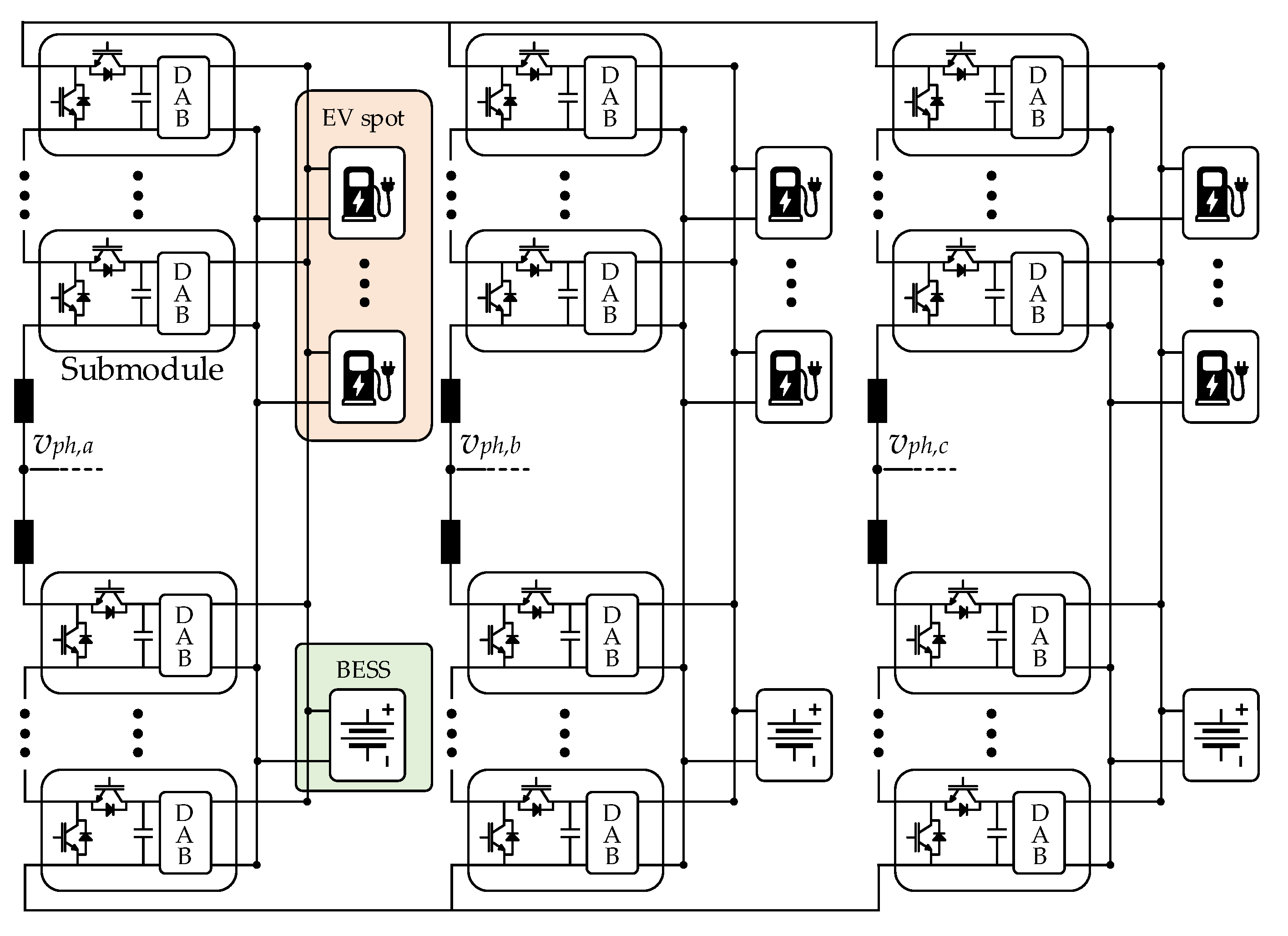
2.1. Overview of the Proposed Charging Station Structure
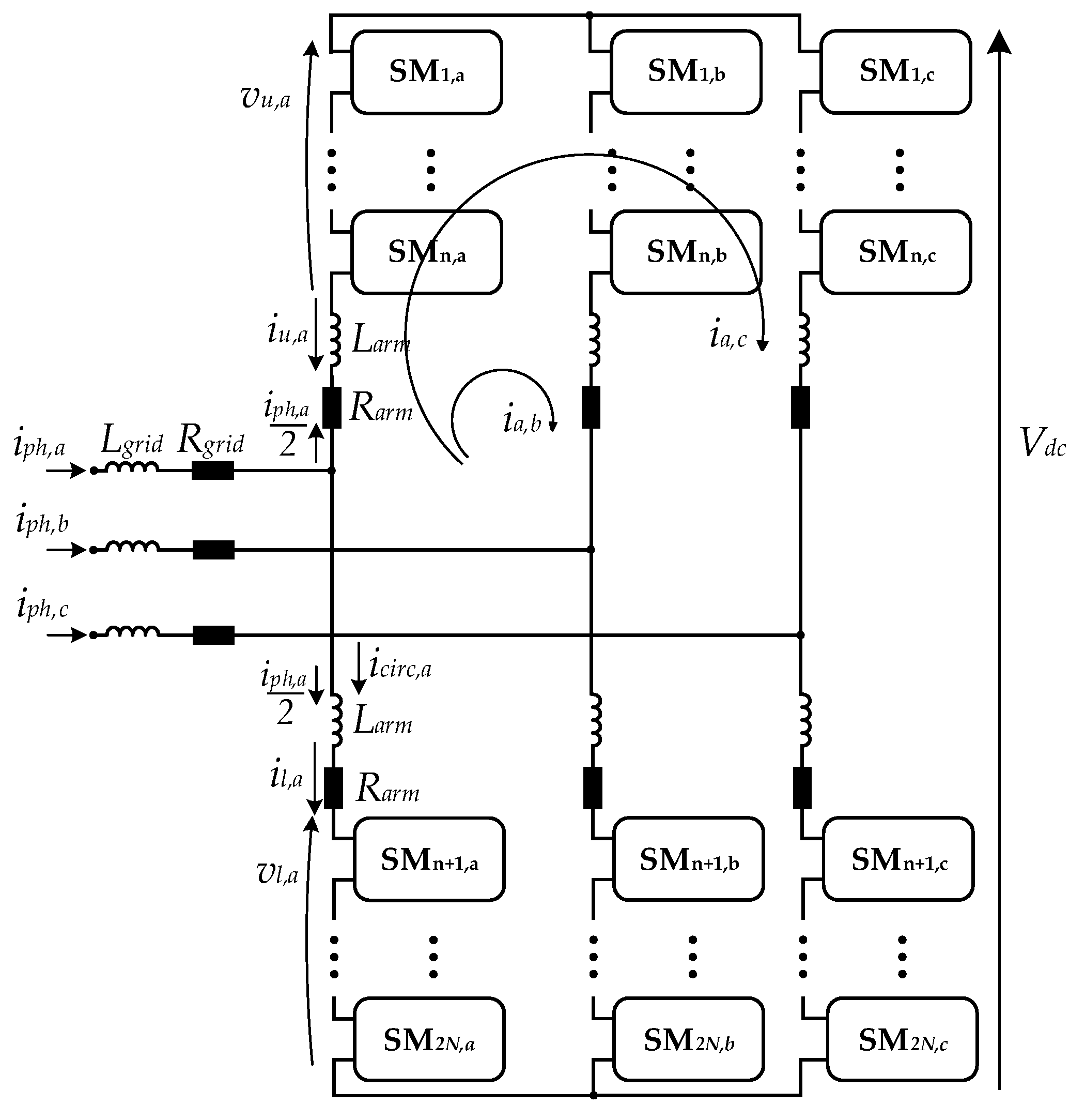
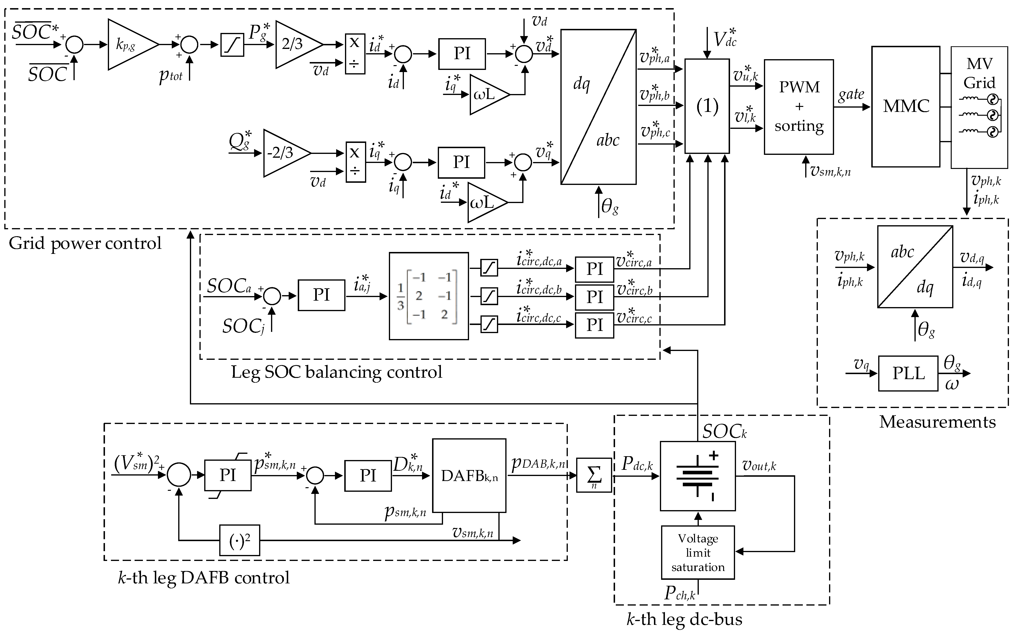
2.2. Modular Multilevel Converter Generalties and Control
2.2.1. Grid Power Control
2.2.2. Converter SOC Balancing
2.2.3. Capacitor Voltage Balancing
- When iu,k ≥ 0, the current is charging the SM capacitors. The capacitor voltages within the arm are sorted in ascending direction. Thus, the least charged capacitors are inserted first.
- When iu,k < 0, the current is discharging the SM capacitors. The capacitor voltages within the arm are sorted in descending direction. Thus, the most charged capacitors are inserted first.
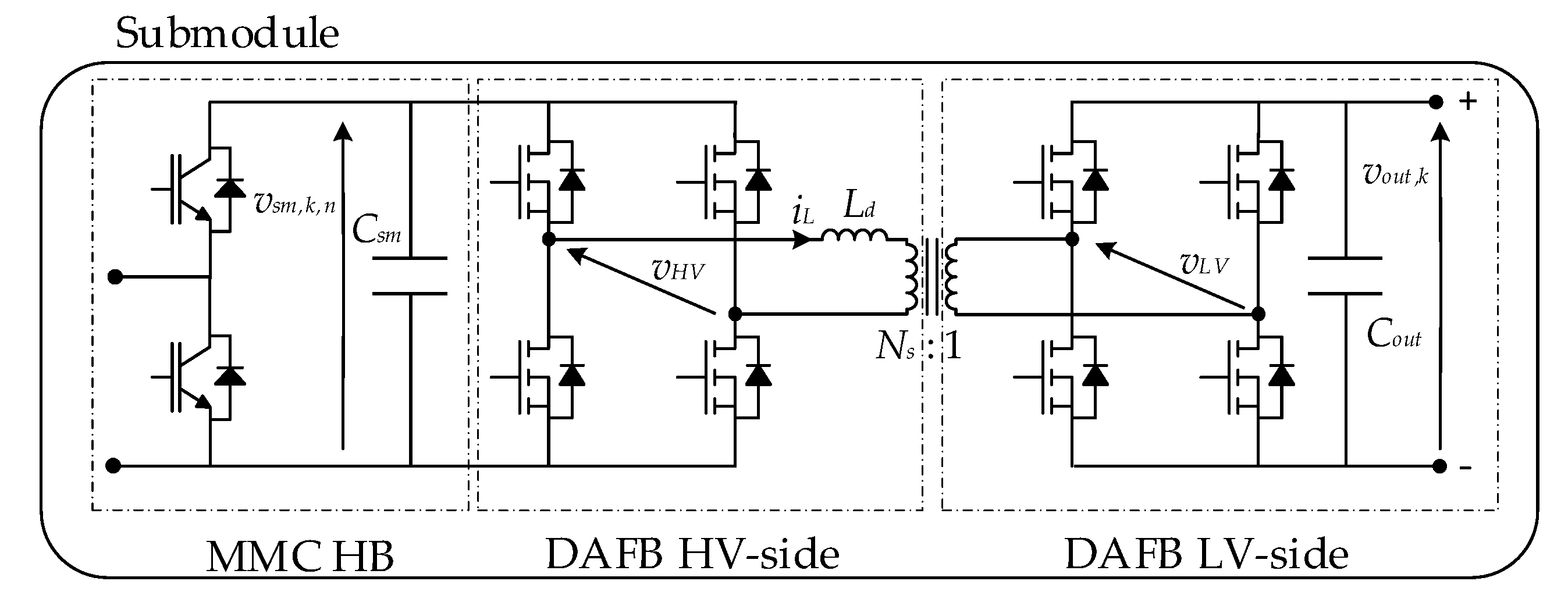
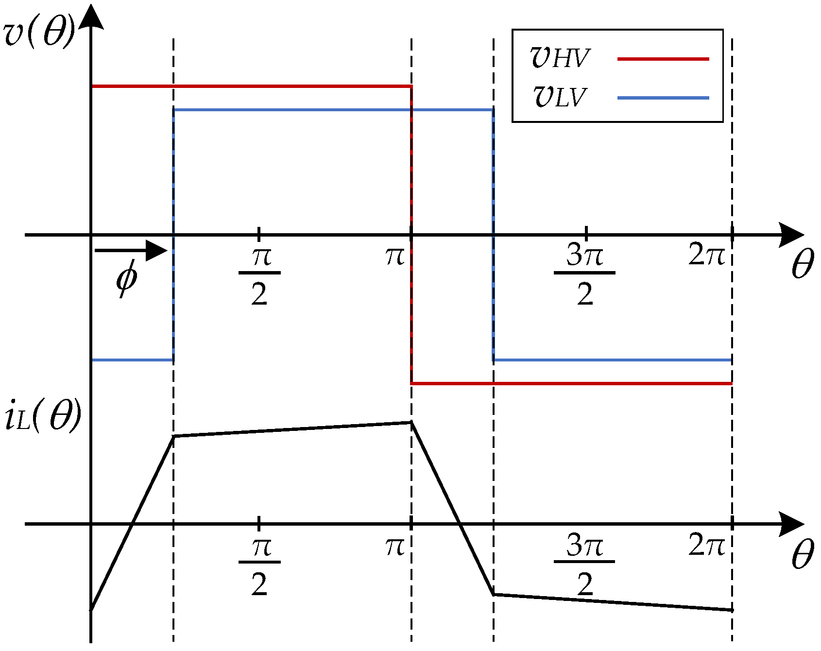
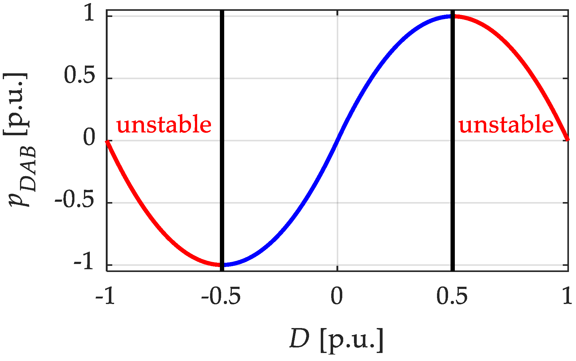
2.3. Dual Active Full-Bridge Control
2.4. Vehicle Charging Control
3. Case Study and Results
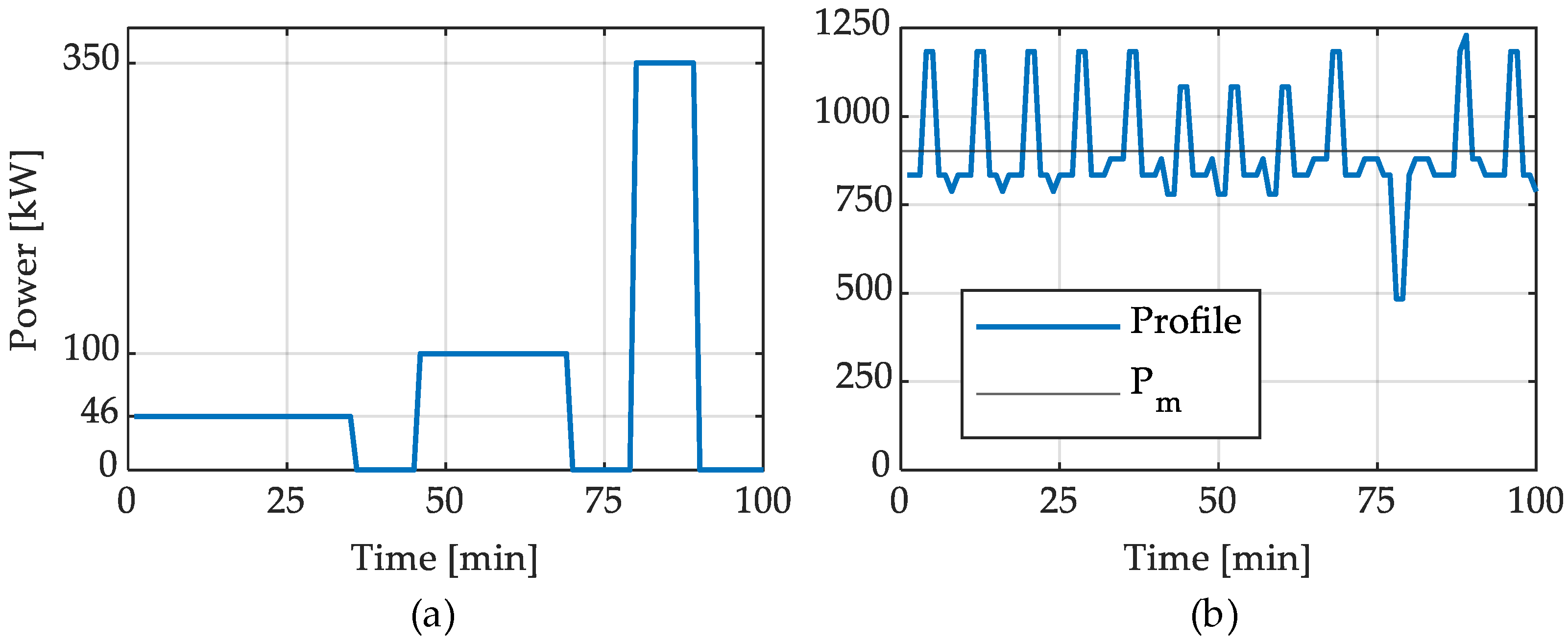
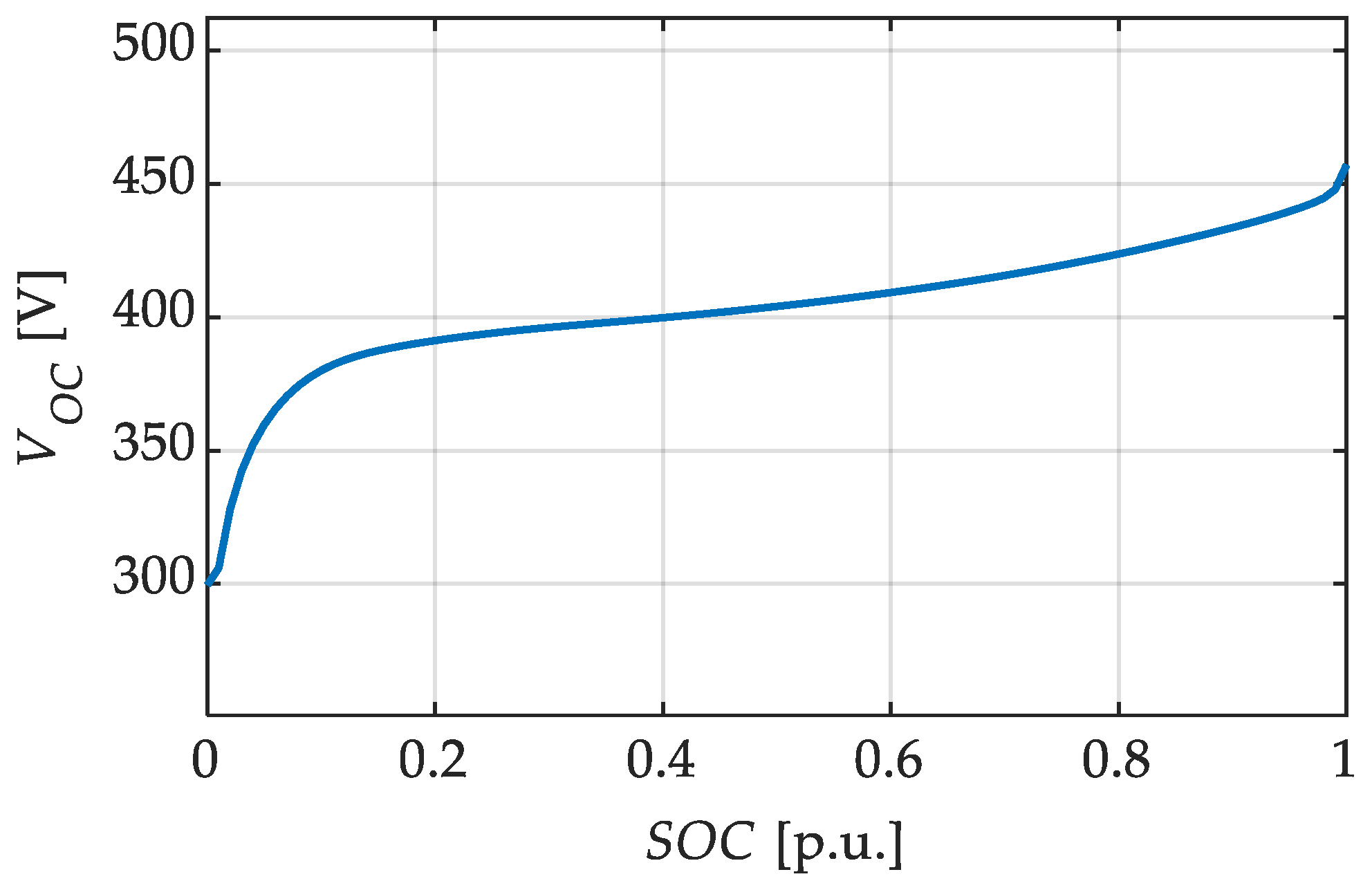
3.1. Charging Station Power Profile and BESS Sizing
3.2. Grid-Side Converter and DAFB Parameter Selection
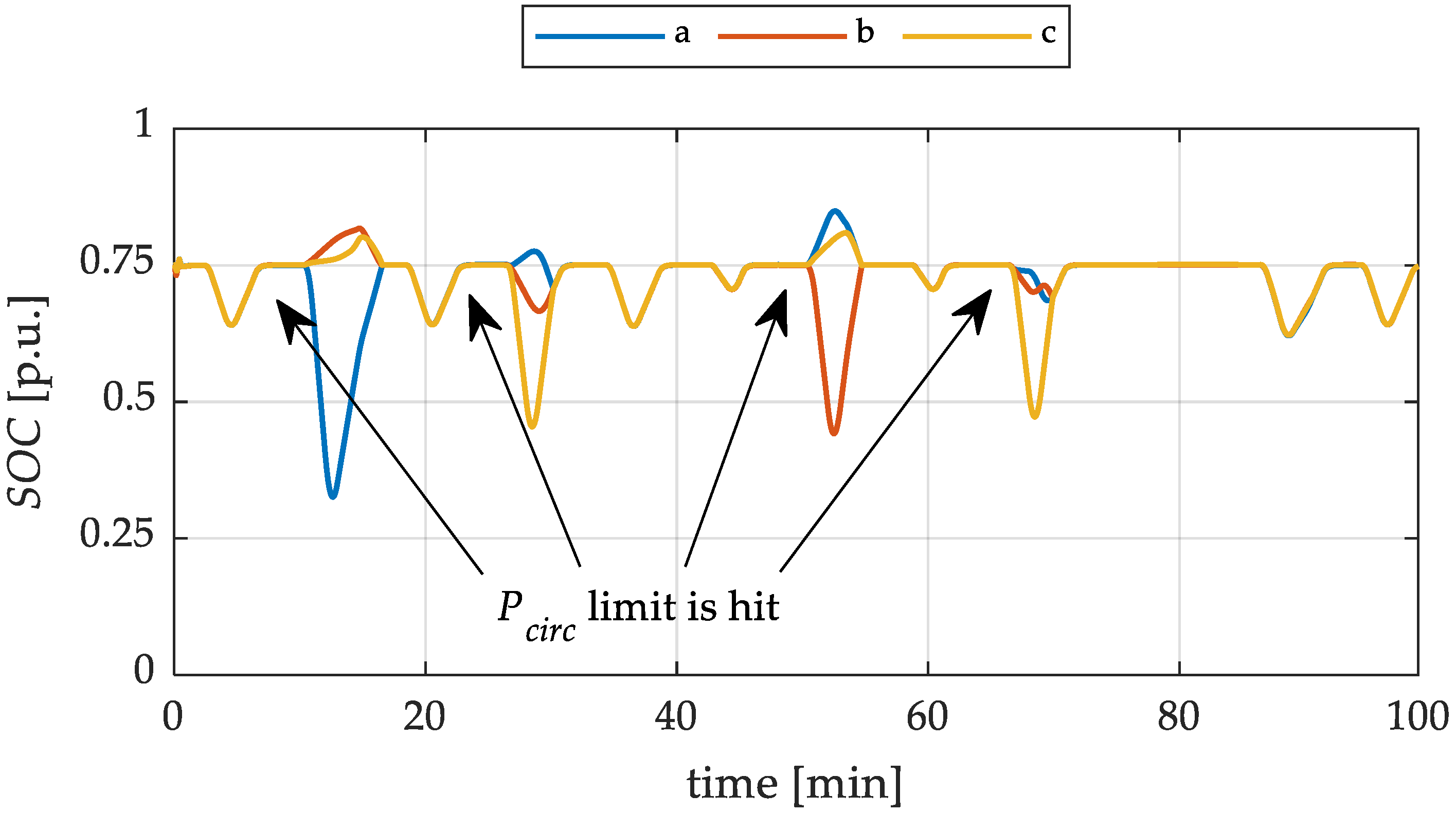
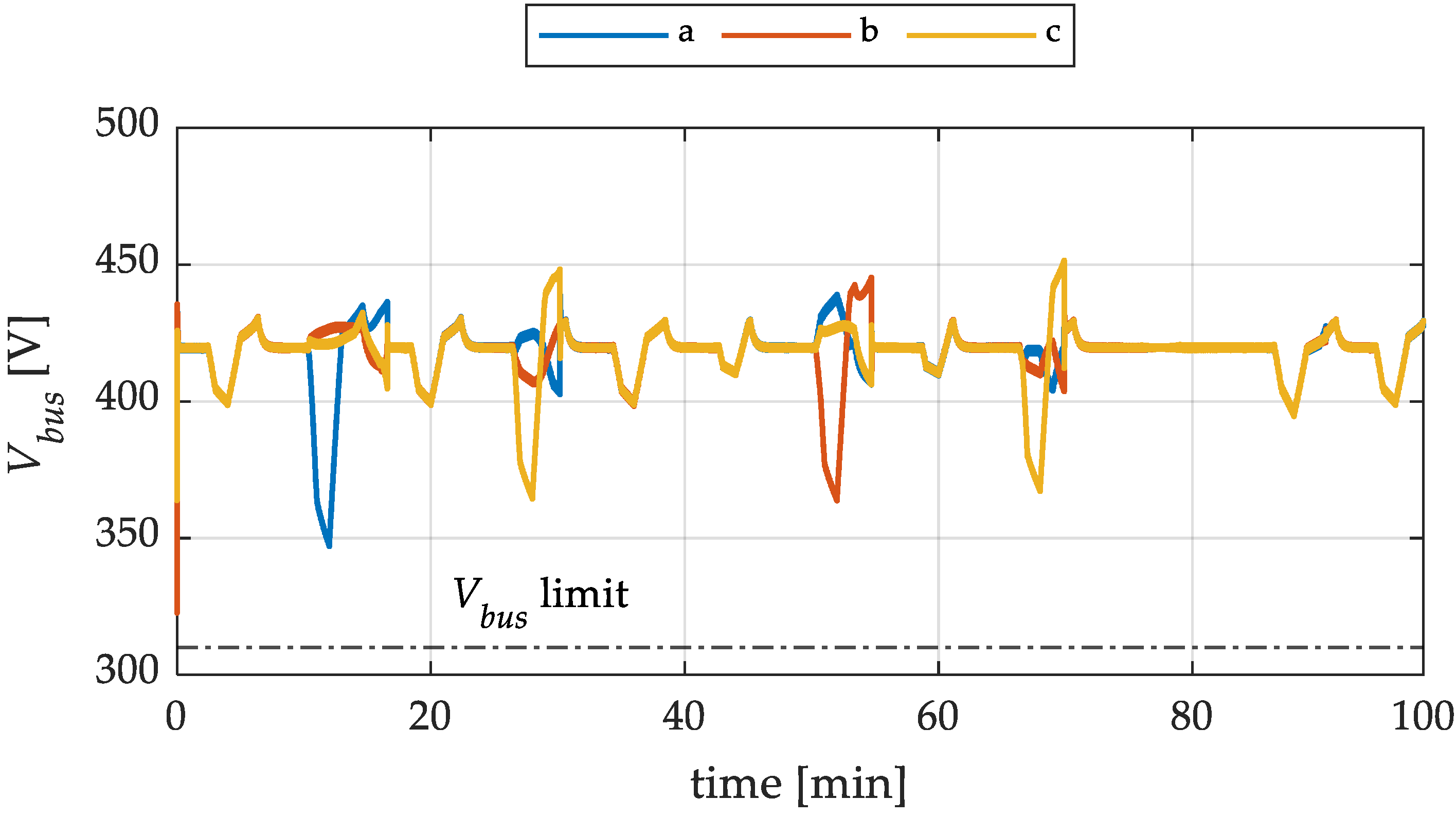
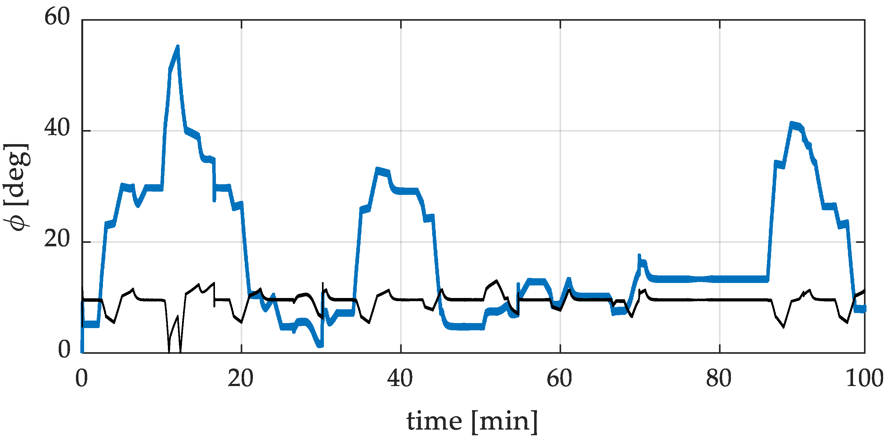
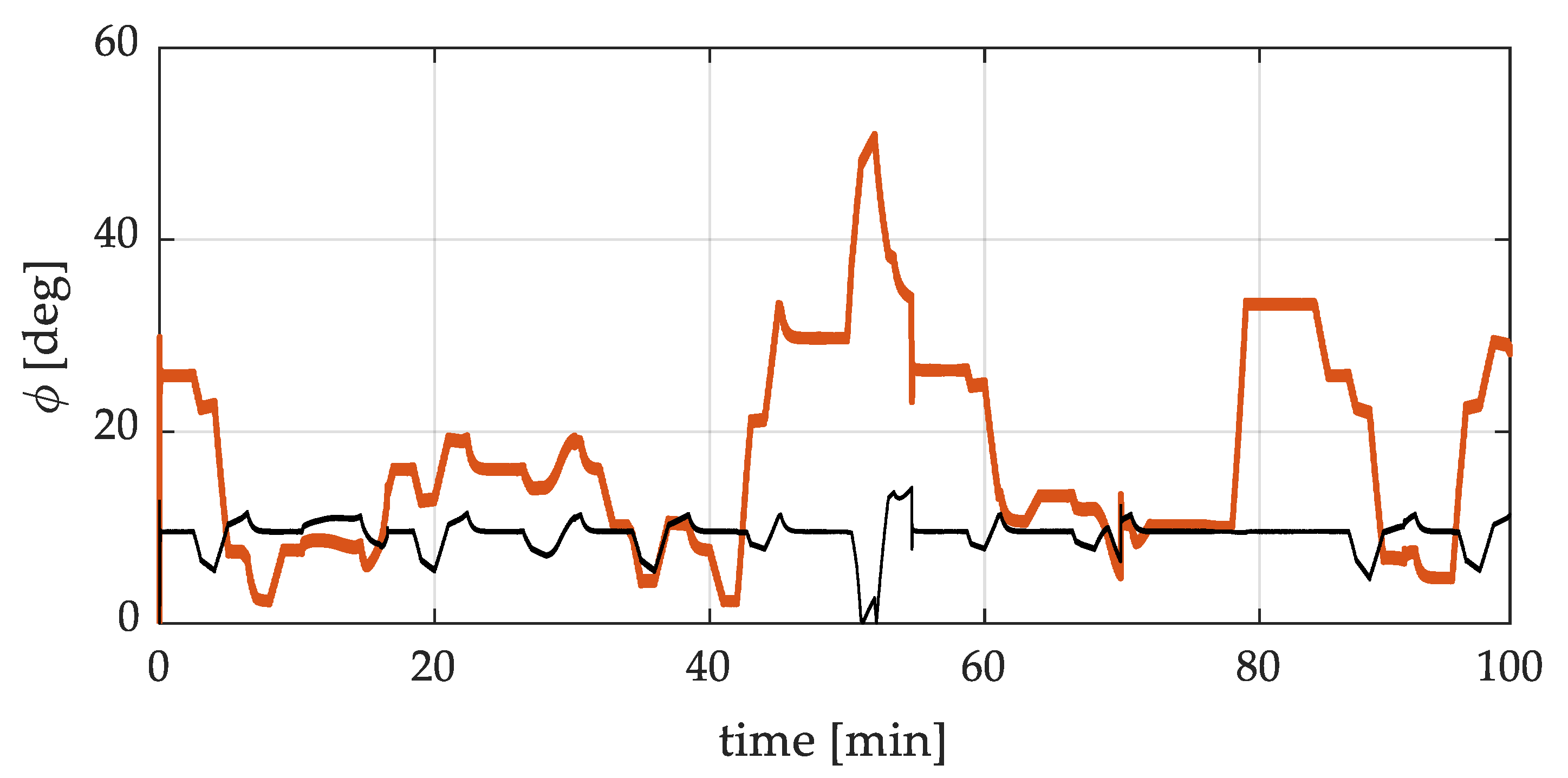
3.3. Simulation Results
4. Discussion
5. Conclusions
Author Contributions
Funding
Data Availability Statement
Conflicts of Interest
References
- Anegawa, T. Development of Quick Charging System for Electric Vehicle. In Proceedings of the 21st World Energy Congress (WEC) 2010, Montreal, Canada, 12–16 September 2010. [Google Scholar]
- Wang, L.; Qin, Z.; Slangen, T.; Bauer, P.; van Wijk, T. Grid Impact of Electric Vehicle Fast Charging Stations: Trends, Standards, Issues and Mitigation Measures—An Overview. IEEE Open J. Power Electron. 2021, 2, 56–74. [Google Scholar] [CrossRef]
- Rahman, M.M.; Oni, A.O.; Gemechu, E.; Kumar, A. Assessment of Energy Storage Technologies: A Review. Energy Convers. Manag. 2020, 223, 113295. [Google Scholar] [CrossRef]
- Hõimoja, H.; Vasiladiotis, M.; Rufer, A. Power Interfaces and Storage Selection for an Ultrafast EV Charging Station. In Proceedings of the 6th IET International Conference on Power Electronics, Machines and Drives (PEMD 2012), Bristol, UK, 27–29 March 2012. [Google Scholar] [CrossRef]
- Srdic, S.; Lukic, S. Toward Extreme Fast Charging: Challenges and Opportunities in Directly Connecting to Medium-Voltage Line. IEEE Electrif. Mag. 2019, 7, 22–31. [Google Scholar] [CrossRef]
- Vasiladiotis, M.; Rufer, A. Analysis and Control of Modular Multilevel Converters with Integrated Battery Energy Storage. IEEE Trans. Power Electron. 2015, 30, 163–175. [Google Scholar] [CrossRef]
- Vasiladiotis, M.; Rufer, A. Balancing Control Actions for Cascaded H-Bridge Converters with Integrated Battery Energy Storage. In Proceedings of the 15th European Conference on Power Electronics and Applications, EPE, Lille, France, 2–6 September 2013. [Google Scholar] [CrossRef]
- Liang, G.; Tafti, H.D.; Farivar, G.G.; Pou, J.; Townsend, C.D.; Konstantinou, G.; Ceballos, S. Analytical Derivation of Intersubmodule Active Power Disparity Limits in Modular Multilevel Converter-Based Battery Energy Storage Systems. IEEE Trans. Power Electron. 2021, 36, 2864–2874. [Google Scholar] [CrossRef]
- Vasiladiotis, M.; Rufer, A. A Modular Multiport Power Electronic Transformer with Integrated Split Battery Energy Storage for Versatile Ultrafast EV Charging Stations. IEEE Trans. Ind. Electron. 2015, 62, 3213–3222. [Google Scholar] [CrossRef]
- Vasiladiotis, M.; Bahrani, B.; Burger, N.; Rufer, A. Modular Converter Architecture for Medium Voltage Ultra Fast EV Charging Stations: Dual Half-Bridge-Based Isolation Stage. In Proceedings of the International Power Electronics Conference, IPEC-Hiroshima—ECCE Asia, Hiroshima, Japan, 18–21 May 2014; pp. 1386–1393. [Google Scholar] [CrossRef]
- Vasiladiotis, M.; Rufer, A.; Beguin, A. Modular Converter Architecture for Medium Voltage Ultra Fast EV Charging Stations: Global System Considerations. In Proceedings of the 2012 IEEE International Electric Vehicle Conference, Greenville, SC, USA, 4–8 March 2012; pp. 1–7. [Google Scholar]
- Barresi, M.; Ferri, E.; Piegari, L. An MMC-Based Fully Modular Ultra-Fast Charging Station Integrating a Battery Energy Storage System. In Proceedings of the 16th International Conference on Compatibility, Power Electronics and Power Engineering (CPE-POWERENG), Birmingham, UK, 29 June–1 July 2022. [Google Scholar]
- Pugliese, S.; Buticchi, G.; Mastromauro, R.A.; Andresen, M.; Liserre, M.; Stasi, S. Soft-Start Procedure for a Three-Stage Smart Transformer Based on Dual-Active Bridge and Cascaded H-Bridge Converters. IEEE Trans. Power Electron. 2020, 35, 11039–11052. [Google Scholar] [CrossRef]
- Wang, D.; Tian, J.; Mao, C.; Lu, J.; Duan, Y.; Qiu, J.; Cai, H. A 10-KV/400-V 500-KVA Electronic Power Transformer. IEEE Trans. Ind. Electron. 2016, 63, 6653–6663. [Google Scholar] [CrossRef]
- Ouyang, S.; Liu, J.; Chen, H. Arm Current Stress Reduction Technique for a Delta-Connected Solid State Transformer Using Zero-Sequence Current Injection. IEEE Trans. Power Electron. 2021, 36, 12234–12250. [Google Scholar] [CrossRef]
- Valedsaravi, S.; El Aroudi, A.; Martínez-Salamero, L. Review of Solid-State Transformer Applications on Electric Vehicle DC Ultra-Fast Charging Station. Energies 2022, 15, 5602. [Google Scholar] [CrossRef]
- Nair, A.C.; Fernandes, B.G. A Solid State Transformer Based Fast Charging Station for All Categories of Electric Vehicles. In Proceedings of the IECON 2018—44th Annual Conference of the IEEE Industrial Electronics Society, Washington, DC, USA, 21–23 October 2018; pp. 1989–1994. [Google Scholar] [CrossRef]
- Ramya, G.; Ramaprabha, R. Design Methodology of P-Res Controllers with Harmonic Compensation Technique for Modular Multilevel Converter Fed from Partially Shaded PV Array. In Proceedings of the International Conference on Power Electronics and Drive Systems, Sydney, NSW, Australia, 9–12 June 2015; pp. 330–335. [Google Scholar] [CrossRef]
- Nasri, S.; Nowdeh, S.A.; Davoudkhani, I.F.; Moghaddam, M.J.H.; Kalam, A.; Shahrokhi, S.; Zand, M. Maximum power point tracking of photovoltaic renewable energy system using a new method based on turbulent flow of water-based optimization (TFWO) under partial shading conditions. In Fundamentals and Innovations in Solar Energy; Springer: Berlin/Heidelberg, Germany, 2021; pp. 285–310. [Google Scholar]
- Soong, T.; Lehn, P.W. Internal Power Flow of a Modular Multilevel Converter with Distributed Energy Resources. IEEE J. Emerg. Sel. Top. Power Electron. 2014, 2, 1127–1138. [Google Scholar] [CrossRef]
- Prieto-Araujo, E.; Junyent-Ferré, A.; Collados-Rodríguez, C.; Clariana-Colet, G.; Gomis-Bellmunt, O. Control Design of Modular Multilevel Converters in Normal and AC Fault Conditions for HVDC Grids. Electr. Power Syst. Res. 2017, 152, 424–437. [Google Scholar] [CrossRef]
- Debnath, S.; Qin, J.; Bahrani, B.; Saeedifard, M.; Barbosa, P. Operation, Control, and Applications of the Modular Multilevel Converter: A Review. IEEE Trans. Power Electron. 2015, 30, 37–53. [Google Scholar] [CrossRef]
- Akagi, H.; Kanazawa, Y.; Koetsu Fujita, A.N. Generalized Theory of Instantaneous Reactive Power and Its Application. Electr. Eng. Jpn. 1983, 103, 58–66. [Google Scholar] [CrossRef]
- Lesnicar, A.; Marquardt, R. An Innovative Modular Multilevel Converter Topology Suitable for a Wide Power Range. In Proceedings of the 2003 IEEE Bologna PowerTech Conference Proceedings, Bologna, Italy, 23–26 June 2003; Volume 3, pp. 6–11. [Google Scholar] [CrossRef]
- De Doncker, R.W.A.A.; Divan, D.M.; Kheraluwala, M.H. A Three-Phase Soft-Switched High-Power-Density DC/DC Converter for High-Power Applications. IEEE Trans. Ind. Appl. 1991, 27, 63–73. [Google Scholar] [CrossRef]
- Garcia-Bediaga, A.; Villar, I.; Rujas, A.; Mir, L. DAB Modulation Schema with Extended ZVS Region for Applications with Wide Input/Output Voltage. IET Power Electron. 2018, 11, 2109–2116. [Google Scholar] [CrossRef]
- Kheraluwala, M.H.; Gascoigne, R.W.; Divan, D.M.; Baumann, E.D. Performance Characterization of a High-Power Dual Active Bridge Dc-to-Dc Converter. IEEE Trans. Ind. Appl. 1992, 28, 1294–1301. [Google Scholar] [CrossRef]
- Arias, M.B.; Bae, S. Electric Vehicle Charging Demand Forecasting Model Based on Big Data Technologies. Appl. Energy 2016, 183, 327–339. [Google Scholar] [CrossRef]
- Li, Y.; He, S.; Li, Y.; Member, S. Probabilistic Charging Power Forecast of EVCS: Reinforcement Learning Assisted Deep Learning Approach. IEEE Trans. Intell. Veh. 2023, 8, 344–357. [Google Scholar] [CrossRef]
- Ahmadi-Nezamabad, H.; Zand, M.; Alizadeh, A.; Vosoogh, M.; Nojavan, S. Multi-Objective Optimization Based Robust Scheduling of Electric Vehicles Aggregator. Sustain. Cities Soc. 2019, 47, 101494. [Google Scholar] [CrossRef]
- Nasab, M.A.; Zand, M.; Padmanaban, S.; Dragicevic, T.; Khan, B. Simultaneous Long-Term Planning of Flexible Electric Vehicle Photovoltaic Charging Stations in Terms of Load Response and Technical and Economic Indicators. World Electr. Veh. J. 2021, 12, 190. [Google Scholar] [CrossRef]
- Directive 2014/94/EU of the European Parliament and of the Council of 22 October 2014 on the Deployment of Alternative Fuels Infrastructure Text with EEA Relevance. Available online: https://eur-lex.europa.eu/legal-content/EN/TXT/?uri=celex%3A32014L0094 (accessed on 21 April 2023).
- ARERA Rapporto Finale Della Ricognizione-Mercato e Caratteristiche Dei Dispositivi Di Ricarica per Veicoli Elettrici. Available online: https://www.arera.it/allegati/pubblicazioni/210503_dispositivi_ricarica.pdf (accessed on 21 April 2023).
- 519-2022; IEEE Standard for Harmonic Control in Electric Power Systems 2022. Institute of Electrical and Electronics Engineers: Piscataway, NJ, USA, 2022.


| Vehicle | Charging Power | Battery Capacity | Charging Time |
|---|---|---|---|
| BMW i3 | 46 kW | 37.9 kWh | 35 min |
| Nissan Leaf e+ | 100 kW | 56 kWh | 24 min |
| Porsche Taycan | 350 kW | 83.7 kWh | 10 min |
| Parameter | Value | Unit |
|---|---|---|
| Minimum BESS energy | 28 | kWh |
| System efficiency ηsys | 0.9 | - |
| Total BESS energy | 45 | kWh |
| Single battery energy Ebatt | 15 | kWh |
| Nominal voltage Vbatt | 400 | V |
| Internal resistance Rbatt | 85 | mΩ |
| Parameter | Value | Unit |
|---|---|---|
| Grid short-circuit power | 190 | MVA |
| Grid line-to-line voltage Vg | 11 | kV |
| Grid frequency fg | 50 | Hz |
| Grid inductance Lg | 2 | mH |
| Grid resistance Rg | 0.113 | Ω |
| Parameter | Value | Unit |
|---|---|---|
| MMC rated active power | 1 | MW |
| Rated SM voltage Vsm | 1500 | V |
| Number of SMs per arm N | 15 | - |
| Rated dc bus voltage Vdc | 22.5 | kV |
| SM capacitance Csm | 20 | mF |
| Arm inductance Larm | 5 | mH |
| Arm resistance Rarm | 1 | mΩ |
| Switching frequency fs,MMC | 3150 | Hz |
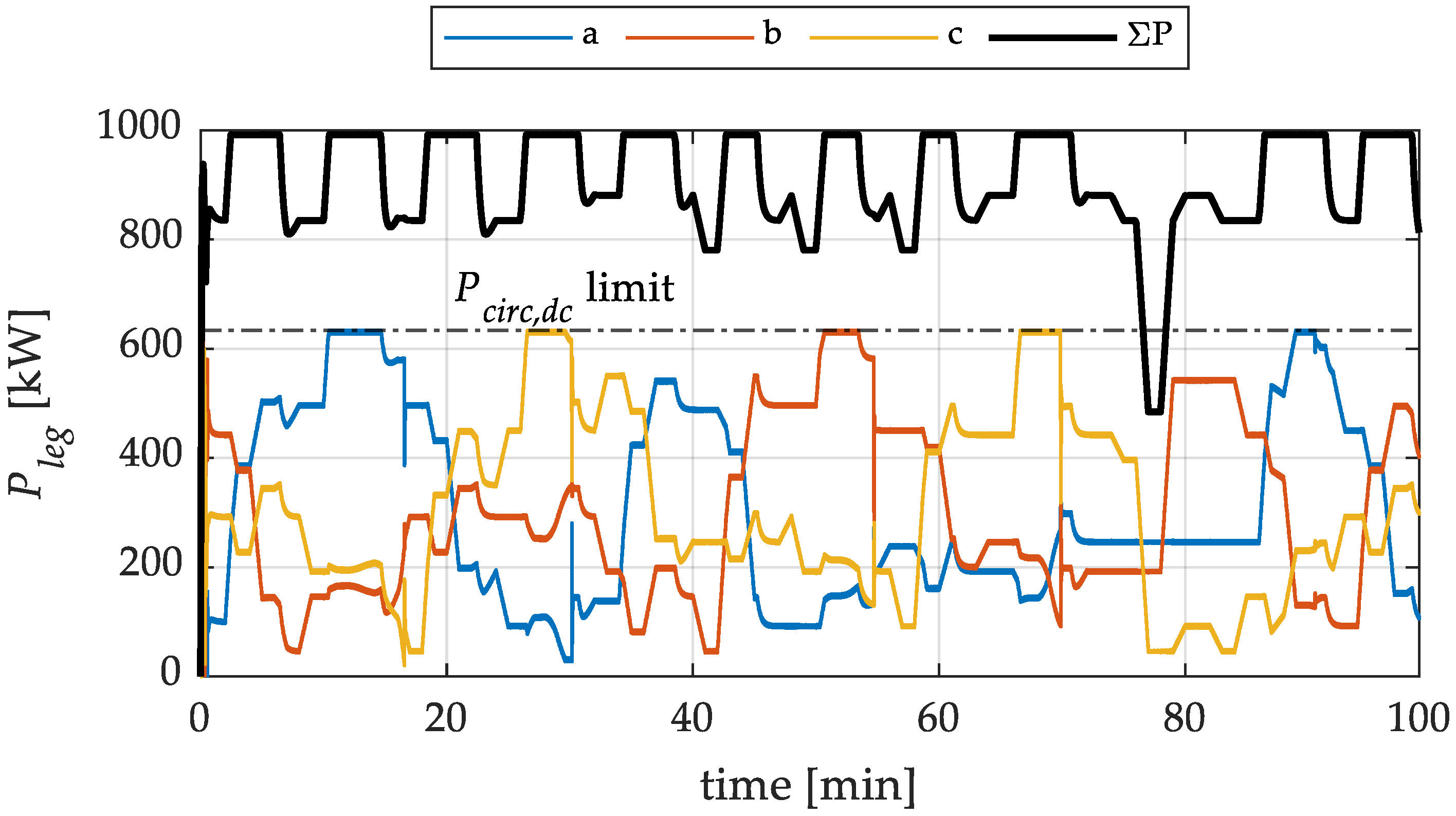
| Maximum circulating power per leg | 300 | kW |
| Maximum circulating current | 13.33 | A |
| Parameter | Value | Unit |
|---|---|---|
| Rated output voltage Vout | 400 | V |
| Minimum dc bus voltage | 310 | V |
| Transformer turn-ratio Ns | 4 | - |
| Switching frequency fs | 50 | kHz |
| Maximum grid power contribution per SM | 11.1 | kW |
| Maximum circulating power per SM | 10 | kW |
| DAB rated power PDAB | 22.15 | kW |
| HV-side leakage inductance Ld | 210 | μH |
| Maximum output power (@D = 0.5) | 28.6 1 | kW |
| 22.15 2 | kW | |
| Output capacitance Cout | 0.65 | mF |
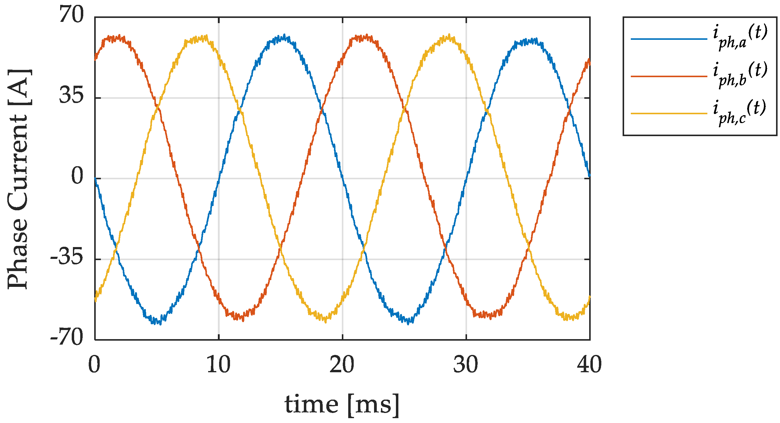
| Current | THD [%] |
|---|---|
| iph,a | 1.44 |
| iph,b | 1.41 |
| iph,c | 1.48 |
Disclaimer/Publisher’s Note: The statements, opinions and data contained in all publications are solely those of the individual author(s) and contributor(s) and not of MDPI and/or the editor(s). MDPI and/or the editor(s) disclaim responsibility for any injury to people or property resulting from any ideas, methods, instructions or products referred to in the content. |
© 2023 by the authors. Licensee MDPI, Basel, Switzerland. This article is an open access article distributed under the terms and conditions of the Creative Commons Attribution (CC BY) license (https://creativecommons.org/licenses/by/4.0/).
Share and Cite
Barresi, M.; Ferri, E.; Piegari, L. An MV-Connected Ultra-Fast Charging Station Based on MMC and Dual Active Bridge with Multiple dc Buses. Energies 2023, 16, 3960. https://doi.org/10.3390/en16093960
Barresi M, Ferri E, Piegari L. An MV-Connected Ultra-Fast Charging Station Based on MMC and Dual Active Bridge with Multiple dc Buses. Energies. 2023; 16(9):3960. https://doi.org/10.3390/en16093960
Chicago/Turabian StyleBarresi, Marzio, Edoardo Ferri, and Luigi Piegari. 2023. "An MV-Connected Ultra-Fast Charging Station Based on MMC and Dual Active Bridge with Multiple dc Buses" Energies 16, no. 9: 3960. https://doi.org/10.3390/en16093960
APA StyleBarresi, M., Ferri, E., & Piegari, L. (2023). An MV-Connected Ultra-Fast Charging Station Based on MMC and Dual Active Bridge with Multiple dc Buses. Energies, 16(9), 3960. https://doi.org/10.3390/en16093960