Abstract
There has been a notable increase in the frequency and severity of extreme events, such as hurricanes, floods, wildfires, and storms. These events, although infrequent, have a significant disruptive effect, causing prolonged outages and compromising essential services, thereby severely affecting customers’ safety. As a result, there is an urgent requirement to enhance the resilience of distribution networks by quickly restoring the loads during and after a disaster. In this regard, this paper reviews the existing studies on black-start service restoration in active distribution systems and microgrids. A comprehensive review is conducted for each aspect of the restoration problem, encompassing various proposed methods and modeling techniques found in the existing literature. The aim of this review is to consolidate the knowledge and findings from previous studies, providing a valuable resource for researchers and practitioners in the field. Also, some key research directions for the future work in this field are recommended for developing more practical and reliable methods.
1. Introduction
A reliable and resilient power supply is of paramount importance for various critical infrastructures such as hospitals, transportation systems, communication networks, and manufacturing facilities. However, disruptions to the power grid due to various factors, such as severe weather events, equipment failures, or even deliberate attacks, often lead to widespread power outages, causing significant economic losses and jeopardizing public safety. On the other hand, the increasing integration of renewable energies and the emergence of the microgrid (MG) concept have brought new possibilities that can improve the resilience of modern power systems. Leveraging this potential, distributed energy resources (DERs), as decentralized sources, can be used to form MGs that can serve the loads during a blackout even when the bulk power system is unavailable [1].
In a contingency scenario, the restoration of the out-of-service loads can be achieved by reallocating the de-energized demand nodes to adjacent and auxiliary feeders [2]. This is achieved by changing the status of tie and sectionalizing switches, which allows the transfer of electrical flow to the desired nodes. The reallocation of the loads is performed using the network-reconfiguration procedures, which take into account the different operational, physical, and topological constraints of the network [2]. The reconfiguration algorithms typically address local outages and component faults by effectively changing the network topology to restore power and mitigate the impact of the disruptions.
In the case of extreme events, such as hurricanes, tornados, and cyberattacks, several outages may happen in the system that can cause major outages, leaving a large region within utility service territories without power. In this case, a black-start restoration procedure is performed to restore power to the loads. Black-start restoration refers to the process of restoring energy to the network following a complete or partial blackout. Black-start restoration is a critical aspect of power-system resilience, enabling the rapid recovery of the power supply in the event of a widespread blackout, and plays a significant role in maintaining the reliability and stability of the power grid.
In this paper, an extensive literature review is conducted focusing on black-start service restoration in ADNs and MGs. Three important features are discussed in the paper: (i) mathematical modeling of different components in the system is reviewed, (ii) different mathematical methods and solution approaches proposed in the literature are discussed and compared to each other, and (iii) some key research directions and gaps are recommended that arise from the inherent characteristics of the black-start restoration problem. This review paper focuses on journal papers addressing the black-start restoration problem which were published from 2016–2022.
Typically, the black-start restoration problem is formulated as a combinatorial optimization problem, necessitating the utilization of advanced computational resources to be solved. In recent decades, the advancements in high-tech computing, along with the emergence of the MG concept and the growing integration of DERs into power systems, have created a viable and realistic environment for proposing novel models and formulations to address the black-start restoration problem. These new approaches offer promising solutions that can be effectively implemented in practical systems, leveraging the improved computational capabilities and benefits of MGs and DERs to enhance the effectiveness of the restoration process.
The rest of the paper is organized as follows. The various formulations of the restoration problem are presented in Section 2 which includes the operational and topological constraints of active distribution networks (ADNs). In Section 3, different methodologies and strategies proposed by the existing literature are reviewed. The different test systems and software tools deployed in the reviewed papers for the black-start restoration problem are summarized in Section 4. In Section 5, the future research areas within the domain are discussed and conclusions are provided in Section 5.
2. Distribution System Restoration Formulation
There are several definitions for resiliency in power systems and other critical infrastructures. However, most of these definitions are focused on the ability of the system to anticipate, absorb, and rapidly recover from an external, extreme, high-impact, and low-probability disturbance [3]. The conceptual resiliency curve, shown in Figure 1, depicts the system-resilience level as a function of time with respect to an extreme event. This curve illustrates the essential characteristics that a power system needs in order to effectively withstand and adapt to changing conditions resulting from an event, such as a hurricane passing through the system. To improve the system resiliency, an action should decrease the green area shown in the figure.
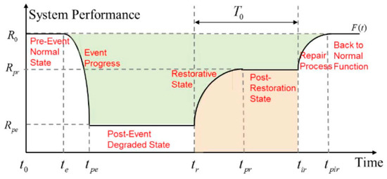
Figure 1.
A conceptual resilience curve of a system corresponding to an extreme event [4].
The black-start restoration problem, which aims to re-energize customers following a major outage, falls in the restorative and postrestoration state. Therefore, the resilience of the system, denoted by R, is defined as (1).
where F(t) is the system performance [4]. In the restoration problem, the resilience can be improved by restoring the system as fast as possible. Accordingly, by defining the system-performance function as the sum of the prioritized loads in service, i.e., , the system resilience can be calculated as (2) [4].
where L is the set of loads and , , and are the priority weight, active power consumption, and in-service duration time of load n, respectively.
2.1. Objective-Function Definition
According to the aforementioned definition of resilience in Equations (1) and (2), maximizing the total restored energy, or equivalently, minimizing the total not-served energy, is a key part of the objective function defined in the existing literature. However, other terms or expressions may be added into the objective function of the restoration problem according to the particular problem and constraints being addressed. The existing literature addressing the black-start restoration problem can be categorized into two main groups in terms of the optimization problem objective function: static and dynamic optimization. In static optimization, the goal of the problem is to maximize or minimize an objective function at the end of the restoration for one instant in time. In static optimization, the key part of the objective is to maximize the total restored load (e.g., in kW) after restoring the system. Therefore, the mathematical formulation of the problem is not concerned about the restoration steps during the restoration procedure. On the other hand, dynamic optimization defines the problem in a step-by-step manner over a period of time, and, hence, the system configuration and performance are tractable during the restoration procedure. Accordingly, the objective function is defined as maximizing the restored energy (e.g., in kWh) which incorporates two important terms, maximizing the total restored load as fast as possible.
2.1.1. Static Objective Functions
In general, the static objective function can be defined as (3) [5].
where is a binary variable representing the energization status of load n. It should be noted that in [6], the objective function was considered as maximizing the total number of restored loads, without including the power demand of the loads. In addition to the above equation, reference [7] considered another term for minimizing the average voltage variation of critical loads as the objective function, and references [8,9] included the minimization of the number of switching actions in their objective function alongside Equation (3). Also, after finding the solution of the service restoration and network configuration at the final stage, if any violation in the power-flow results happened, a network-reconfiguration stage was considered in [9] to optimize the power flow and reduce the flowing power through the lines if the operational constraints of the system are violated. The objective function of this stage was defined to minimize the flowing apparent power in the highly loaded line, considering the lines’ maximum capacity.
where B is the set of branches (lines) and and are apparent power through branch k and maximum capacity of it, respectively.
The authors in [10], proposed a two-stage framework for what it terms critical service restoration, using a microgrid formation framework to reach the following goals: ensuring the restoration of critical loads and maintaining a high survivability in extreme events. In the first stage, the microgrid topology and resource allocation are defined by minimizing the not-energized critical loads. The second stage is utilized to reconfigure the network, reposition the mobile energy sources, and shrink the microgrids to decrease the loss of critical loads in an extended extreme event. In this regard, the objective function is to minimize the number of restored lines and minimize the difference between the number of microgrids and a number of loops in the system. A weighted-sum approach was then used to gather the three objective functions, in which the weight of the first stage is set to a large value to prioritize reducing the not-served critical loads.
2.1.2. Dynamic Objective Functions
A dynamic objective function for a restoration problem can be typically defined as (5) [4,11,12,13,14,15,16,17,18,19,20,21,22,23,24,25,26,27].
where is a binary variable representing the energization status of load n at time step t, and is the duration for each step of restoration (which can be a fixed value or variable based on the considered restoration model).
Furthermore, the authors in [19] addressed the routing and scheduling of repair crews (RCs) and mobile power sources (MPSs) dispatched for the restoration problem. In this regard, they incorporated the following expression into the abovementioned objective function.
where is the weight of this term in the objective function and is considered to be small enough so that the first expression (i.e., maximizing the total restored load) is still dominating, and are the sets of repair crew teams and mobile power sources, and and are binary variables which equal to one if RC k and MPS s are traveling on the transportation system, and equal to zero if RC k and MPS s are visiting one of the nodes in the system. The second term is added to the objective function for two main reasons: to avoid traveling of the RCs and MPSs after all the loads are restored, and to select a dispatch strategy with a minimum number of travels of RCs and MPSs when there is more than one dispatch strategy that can achieve the same optimal service-restoration scheme. A similar formulation of the objective function was used in [24] to minimize the travel time of RCs and MPSs. However, instead of (5), maximizing the cumulative service time for loads was considered in [24] (and [4]), which can be represented as (5) by eliminating the active power of the loads. Reference [17] also addressed the RC dispatch problem using a two-stage framework. The objective function of the RC routing was considered as minimizing the distances between depots (which are centralized locations where RCs are stationed to respond to failures and outages) and damaged components. Also, a term was added to the distribution-system restoration stage to ensure that all damaged components are repaired in a time-efficient manner. In order to incorporate the operational cost of the supplying units during the restoration procedure, the authors in [25] subtracted the cost of operating the MPSs from the objective function of (5). Similarly, reference [20] incorporated three different cost functions corresponding to PV real power curtailment cost (which is proportional to the difference between the total capacity of the PV and its real power generation at each time step), microturbine (MT) operation cost, and line-loss cost (which is proportional to the line losses in the system).
A complementary formulation for the objective function (5) has been defined as minimizing the not-served energy to the loads [28,29,30,31,32,33]:
The summation of the total restoration time was added to the objective function in [28] to consider accelerating the restoration procedure. The authors in [33] proposed a sequential service restoration considering virtual power plant (VPP) scheduling. The objective function for the VPP scheduling problem was considered to minimize the active and reactive power-consumption deviation from the given set points and the operation cost of DGs and maximize the achieved revenues from the demand response and electric vehicle (EV) charging load. Also, the objective function for the restoration problem in [33] was to minimize the unserved load (as defined in (7) by considering the summation of the active and reactive powers of the load for the load demand), power consumption in VPPs, and power-generation cost over the studied time horizon.
In [34], the authors proposed a graph reinforcement learning (G-RL) based algorithm to learn effective control policies for the service-restoration problem sequentially. In this work, the reward function was defined as the total restored energy in the system. Also, the reward function was heavily penalized by power flow violation and loop formation during the restoration procedure.
2.2. System-Component Modeling
Effective power-system restoration requires a detailed understanding of the behavior and interdependencies of various system components. In this section, the different models of loads, DGs, and DERs, which have been used in the literature, are discussed.
2.2.1. Load Modeling
Generally, the load modeling approaches can be categorized into two main groups: static models and dynamic models [35]. In static modeling, the consumed power of the load is represented as a mathematical function of voltage and/or frequency and consists of constant impedance, constant current, and constant power components. On the other hand, dynamic models imitate the dynamic behavior of the loads by considering their dependence on time. Usually, the dynamic models are used to describe the behavior of motor loads and the inrush characteristics of cold loads [35].
The constant power model is the most commonly used load modeling and is utilized in most black-start restoration methods [4,5,6,11,15,16,18,20,23,24,26,28,31,32,34,36]. Based on this model, the active and reactive power consumption of the load is considered to be constant during the restoration procedure and independent of the load voltage and system frequency. Also, in some papers, the specific load model being utilized is not explicitly mentioned [7,8,9,10,17,19,21,22,25,27,29]. Furthermore, the ZIP model combines the constant impedance (Z), constant current (I), and constant power (P and Q) components of the load [13,14,30,33]. In this modeling, the active and reactive powers of the load are represented as a polynomial function of the voltage magnitude [14]:
where, is the load demand at the nominal voltage , is the load voltage, , , , , and are constant coefficients representing the percentages of the constant impedance, constant current, and constant power components of the load. The ZIP model in [37] was further broadened to consider a frequency-dependent model for the loads by multiplying (1) by the factor , where, is the nominal frequency, is the bus frequency, and is the frequency sensitivity parameter of the load.
One of the crucial aspects of the dynamic behavior of loads is the cold load pickup (CLPU) phenomena which can challenge the obtained solutions to the black-start restoration problem. CLPU is the additional demand of a load that takes place when the load is reenergized following an extended outage. This excess-demand condition, which is mainly caused by the loss of load diversity in thermostatically controlled loads (TCLs) or the inherent transient behavior, can result in tripping the protection devices during the restoration procedure. There are several models proposed in the literature to estimate the dynamic behavior of the loads under CLPU conditions. Reference [38] provides a comparative study of different modeling approaches. A typical delayed exponential CLPU curve has been considered in [11,17,20,21,39] for the black-start restoration problem. Figure 2 [11] represents the load demand, considering the CLPU condition when a system goes through a blackout at t0, and the restoration procedure picks up the load at t1 with undiversified factor SU. Then, the load demand decreases as the diversity increases until the diversified loading factor SD.

Figure 2.
The delayed exponential demand of a load under CLPU condition [11].
In the proposed restoration procedure [11], the load-demand factor change between two consecutive time steps can be determined as (9).
where can be calculated according to Figure 1 as (10).
where is the time constant of the CLPU model, is the step function, and is the duration between the time step that the load starts gaining diversity and the tth time step. Using this information, the active and reactive power of the load can be calculated under the CLPU condition in an accumulative manner. To do so, can be replaced with and by choosing the corresponding undiversified and diversified loading factors for the active and reactive powers of the load, respectively. Then, the active and reactive powers of the load considering CLPU are calculated in a cumulative way using (11).
where and are load pre-event active and reactive powers, and is a binary variable representing the energization status of the load at time step t.
It should be noted that these calculations are applicable when there is an extended outage in the system, meaning that the diversity of TCL operating states is completely lost, and the TCLs have the same initial operating state. However, with the emergence of advanced distribution-management systems (ADMS) and using distributed energy resources along the system to enable the black-start and self-healing capabilities of the system, the outage systems may be restored soon after an event happens. In this situation, the CLPU curves of the loads are dependent on the outage time, as shown in Figure 3. In this regard, a time-dependent CLPU model was proposed in [21] to represent the actual dynamic behavior of the loads in the system.
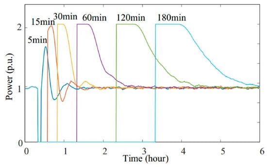
Figure 3.
The CLPU curves under different outage times [21].
In addition to the mentioned dynamic load models, some studies considered the demand response (DR) in the black-start service-restoration problem [12,18,33]. In [18], the authors proposed a time-dependent method to find the minimum and maximum value of each household connected to a bus in order to find the load-demand range in each bus. To do so, an optimization-based model was utilized to be implemented at the household level considering the outage duration. Different smart appliances, including thermostatically controlled loads, deferrable loads, solar generation, and energy storage, were modeled in this work. Then, the minimum demand level of each bus is determined, such that it minimizes the load consumption at the household level and considers the customers’ comfort level. Also, the maximum demand for each bus was considered to be the forecasted load demand. According to the load-demand range for each bus, the black-start restoration problem can be implemented in the system considering the flexibility in the load consumption. Based on the provided results, the amount of restored load during and after the service restoration can be significantly improved using the DR and flexibility in the load demand. However, the effect of DR in the restoration problem is closely related to the location of the controllable buses.
Reference [33] modeled the three-phase DR load in virtual power plants (VPPs). A VPP is a web-based controlled power plant that aggregates the capacities of distributed energy resources (DERs) and local load demands flexibility for trading in energy markets [40]. The revenue of the load-demand response in [33] is divided into several parts, and a fixed energy price is considered for each part. Then, the DR revenue for each flexible load in a VPP is modeled as a piecewise linear function, and the actual active power of the loads in a VPP is the summation of these parts. It should be noted that a fixed power factor is considered to calculate the reactive power for each part.
In all the aforementioned load models, it is assumed that a forecasted value is available for the load demand in the system. However, the demand value has a degree of uncertainty which can affect the obtained solutions in the real-world application. More specifically, there is a high degree of uncertainty in load demand in the black-start restoration problem, since the system has experienced an outage, and the forecasted demand is subject to high uncertainty. In this regard, a few works have addressed the uncertainty of system loads in the restoration problem using different methods [7,8,18,21,33]. In [18], a scenario-generation procedure, based on their prior work in [41], has been utilized to address the uncertainty in the loads. According to this method, a scenario tree is developed which represents the possible values for the uncertain value. To construct this finite tree, the load demand is sampled based on the normal distribution.
In [8], the uncertainty in load demand was modeled using the scenario-generation method based on prediction intervals (PIs). A PI is an interval in which the future observation will fall within a certain probability.
In [7], the uncertainty of load demand was implicitly considered in the availability of each microgrid to supply critical loads in the system. In this regard, the concept of continuous operating time (COT) was introduced for each microgrid to assess the availability of a microgrid for service restoration. The COT of a microgrid refers to the expected maximum duration for which the microgrid can consistently supply its local critical load based on the available generation resources. A microgrid can participate in a restoration procedure if and only if its COT is more than the entire outage time of the system. The α-percentile of the COT is defined as (12).
where is the maximum duration for which the microgrid can serve critical loads in restoration mode, Pr stands for the probability, and α is a predefined probability level. represents the overall level of , and, according to the above equation, is greater than in most of the cases. To integrate the uncertainty modeling into the problem, this work used a chance-constrained approach and utilized sample average approximation (SAA) to transform the chance constraints into deterministic ones.
Reference [33] also used the chance-constrained approach to address the uncertainty in load demand. A distributionally robust approach for chance constraints was proposed in this work, considering that the probability distributions of uncertain parameters are not fully known. This reformulation guarantees that the solution remains robust regardless of the specific uncertainty distribution, which is defined within a moment-based ambiguity set.
In [21], a robust method based on the information gap decision theory (IGDT) was utilized to consider the load uncertainty in the restoration problem. The IGDT-based method models the uncertainties by uncertainty sets without requiring the probability distribution. Also, the envelop-bound model, which is the key part of an IGDT method, was deployed to characterize this uncertainty according to (13).
where b is the uncertain parameter, b0 is the uncertain parameter nominal value, and μ is the extent of the fluctuation. Then, the IGDT-based restoration problem is formulated in such a way that maximizes the allowed fluctuations in the load demand, and, hence, the obtained solution by the proposed method is robust to the worst case, which is the situation when the load fluctuation is at the maximum.
Table 1 summarizes the load modeling approaches utilized in the literature.

Table 1.
Summary of the load modeling approaches.
2.2.2. Generator Modeling
Distributed generators (DGs), usually referred to as power generation near the point of consumption, and renewable energies, such as PV and wind turbine (WT), play a key role in the black-start restoration problem, as they are the only power source to supply the loads in the absence of main grid power. Based on the literature, DG modeling can be broadly categorized into two main categories: steady-state modeling and dynamic modeling.
Steady-state modeling, which is also referred to as PQ modeling, primarily focuses on the steady-state behavior of DGs within the distribution system. References [5,7,15,16,17,29,34] employed a PQ model that constrained the output power of DGs within a defined range, encompassing both minimum and maximum values. A similar model was used for mobile emergency generators (MEGs) which were dispatched as DGs to some nodes in the ADNs [19,31], as well as PVs and microturbines (MT) [20,25]. Furthermore, DG output ramp rate [4,6,8,9,11,12,13,14,18,21,22,24,27,28,30,32,33] and frequency response rate (FRR) [9,11,14,18,30,32] constraints have also been considered in the literature, which can be formulated, respectively, as (14) and (15).
where is the maximum allowable ramp rate for DG g, is the active power output of DG g at time t, G is the set of DGs, and is the FRR factor, which is the maximum allowable incremental restored load and is defined based on the total rated generation capacity in the system.
Distribution systems and microgrids are inherently unbalanced mainly because of their single- and two-phase loads and laterals. Hence, the unbalanced operation of the DGs was addressed in a few works using current unbalance factor (CUF) constraint [14,18,22,26,28,33] and/or output power unbalance mitigation [12,13,28,33]. The CUF is defined as the ratio of the negative sequence current to the positive sequence current at the first harmonic.
where , , and are phase a, b, and c currents. Three-phase synchronous DGs will trip when the CUF is larger than 20%. However, inverter-based DGs are able to operate up to 100% CUF [14]. As is clear, Equation (16) is a nonconvex, nonlinear equation. The interested reader is referred to [14,28] for details on how to linearize this equation. On the other hand, linear constraints such as (17) and (18) can be used to maintain the phase unbalance of the DGs in an acceptable range [12,13,28].
where and are the active and reactive powers of DG g at time t and phase , respectively, and and are the maximum acceptable active and reactive power outputs of the DG. It should be noted that (17) and (18) are considered for the DGs which provide a reference point for the frequency and/or voltage in the system.
On the other hand, dynamic modeling considers the transient and dynamic responses of DGs during the restoration procedure. This model is crucial for ensuring the reliable and secure operation of the system under dynamic conditions, aiding in the development of effective control and protection strategies. In this regard, the frequency response characteristic of grid-forming DGs is studied in [28]. In this work, it is assumed that each formed microgrid is equipped with a three-phase synchronous diesel generator with an isochronous governor. Accordingly, for an instantaneous change in the electrical power from to at t = 0, the differential change in rotor speed in Laplace form is calculated as (19) and (20), which is represented in the standard second-order transfer function.
where is the generator inertia constant in seconds and and are the gains of the integral and proportionate controller, respectively. and are the damping factor and natural frequency in the standard second-order transfer function. Considering , and , and taking the inverse Laplace transform; the frequency change (p.u.) in the time domain is as (21) [28]
Assuming that the transient settles down when the frequency deviation is less than 0.01 Hz, a linear approximation can be derived for the minimum frequency observed in the transient versus the incremental loading , and the slope of this function determines the frequency response rate (FRR) and is used in the FRR constraint. Moreover, a cubic relationship can be obtained for the settling time of the transient versus the incremental loading , which was used to determine the safe time interval that should be observed between switching actions in the restoration procedure. Accordingly, the time interval between switching actions can be defined as (22).
where, is the incremental change in the output of a grid-forming DG. It should be noted that a piecewise linear approximation was used in [28] to linearize the cubic function f. Using (22), the total required restoration time for each formed microgrid using grid-forming DG g can be calculated in a cumulative manner as follows. Then, the total restored time of the formed microgrids can be defined as follows.
Reference [27] proposed a two-level optimization method for the black-start restoration model. In the second level, they utilized the standard outer droop-control structure for each grid-forming unit to model the frequency response of the DG. Since the frequency is mainly controlled by the grid-forming DGs, the maximum frequency drop in the system can be observed by tracking the dynamic behavior of grid-forming DGs; (24)–(30) represent a detailed seventh-order model of the transient behavior of the DGs where the standard outer droop control together with the inner double-loop control structure are adopted [27].
where, , , and are the power controller filter cut-off frequency, nominal frequency, and set point of the frequency controller in rad/s, respectively; and are set point of the voltage controller and bus voltage, respectively; and are the aggregate resistance and inductance of the connection, respectively, as seen by the inverter terminal; and are the restored active and reactive load; and are active and reactive power droop coefficients, respectively; and and are dq-axis values of the DG output current. By solving (24)–(30), the minimum frequency of the DG can be obtained. Then, (31) and (32) were added to the first level, which is the service-restoration problem, to ensure a frequency stable operation of the system.
where, is a binary variable representing the energization status of DG g at time step t; is a hyperparameter representing the virtual frequency-power characteristic of the IBDG; is the maximum allowable change in the active power output of the DG g; is the minimum frequency obtained from the simulation level; and is the minimum allowable frequency. According to (32), the total output of the DG is limited by the maximum allowable change at each time step.
In [12,13], a droop-control-based control method was proposed to coordinate the output of grid-forming DGs (masters) to form a single multimaster MG. The control variables for the reference active and reactive power settings of the droop-controlled inverters are computed to achieve the optimal values at each stage. Subsequently, these optimized reference values are transmitted to the droop-controlled inverters and established during each restoration step. This ensures that the actual power output of the inverters closely aligns with the specified reference settings, maintaining an operation that approximates the desired reference conditions.
Reference [10] constrained the amount of picked load at each load-switching action using the analysis provided in [42]. Accordingly, when a sudden power loss of size (MW) happens in the system with an inertia of () and an individual governor ramp rate of (MW/s), the frequency can be kept above the minimum acceptable frequency if the total governor primary response reserve (MW) is enough to meet .
To determine the maximum allowable load size that can be picked up at each step, (34) can be used for each formed microgrid [10].
In [4], a transient simulation using PSCAD/EMTDC was performed after energizing each load to ensure that the transient voltage, current, and frequency of the DGs are in an acceptable range. The authors used a greedy method in which loads are energized one by one based on their priority level, and if a violation is observed, the corresponding load is removed from the restoration plan. A similar approach was implemented in [23] using GridLAB-D software to check the transient feasibility of each restoration path obtained by their proposed heuristic method.
2.2.3. Energy Storage Systems and Electric Vehicles
Energy storage systems (ESSs) have the potential to offer exceptional flexibility to ADNs due to their ability to strategically generate and absorb power. In [11], (35)–(46) were considered to model the ESS operation, assuming that an ESS can adjust its active and reactive powers, and the state of charge (SOC) of the ESS is not affected by dispatching the reactive power. SOC refers to the current level of energy stored in the battery of an ESS.
where, , , , , , , , and are the minimum and maximum active and reactive powers of ESS e in charging (superscript C) and discharging (superscript D) modes; and are binary variables representing the charging and discharging status of ESS e at time step t; , , , and are active and reactive powers of ESS s at time step t in charging and discharging modes; is a binary variable representing the energization status of the node to which ESS e is connected at time step t; and are the charging and discharging efficiency of ESS s; , , and are the initial, minimum, and maximum percentage of energy for ESS s, is the rated energy capacity of ESS s; and , , , and are active and reactive power ramp rates of ESS s in charging and discharging modes. Constraints (35)–(38) limit the output active and reactive power of the ESS in the charging and discharging modes. Based on (39), an ESS is only allowed to start either charging or discharging when the connected node is energized. The SOC of the ESS is calculated using (40) and constraint (41) keeps the value of the SOC in an acceptable range. Constraints (42)–(45) maintain the charging and discharging ramp rates in a range. Constraint (46) aims to avoid the ESS from excessively charging or discharging continually after the final time step. It should be noted that this paper did not consider the energy loss of charging or discharging of an ESS.
Reference [8] considered only (41) in their restoration method. In [22], constraints (35), (36), and (39)–(41) were used to model the ESS. Also, reference [26] modeled the ESS based on (35)–(41), and reference [25] modeled the ESS using (35), (36), and (39)–(41). Furthermore, reference [33] used (47)–(51), along with (35), (36), (40), and (41) to model the ESS.
where, D/C stands for the discharge or charge mode of operation; is the energy loss of ESS e at time step t; is the per unit resistive losses; S represents the apparent power; , , and are the capability curve coefficients; pf stands for the power factor; and is the permissible active and reactive power phase difference of ESS s. Constraint (47) defines the energy losses of the ESS, and this value is then subtracted from the SOC calculation in (40). The apparent power of the ESS is defined as a piecewise linear function of active and reactive powers, as represented in (48). The operation power factor is enforced by (49), and the balance operation of the ESS is ensured by (50) and (51).
In [15], the authors used mobile battery-carried vehicles (MBCVs) to supply critical loads, especially those in islanded areas of the system. Once a critical load is restored, the MBCV will travel to the location of other critical loads to supply additional loads; (52)–(56) were used in [15] as the operational constraints of an MBCV connected to a node in the system and included in the restoration model.
where, is a binary variable which represents if MBCV e is connected to power station i at time step t; and are binary variables that indicate if MBCV e arrives at and leaves station i at time step t, respectively; is the discharge power of MBCV e in station i at time t; and is its maximum permissible value. It should be noted that constraint (52) ensures that if the MBCV has either left or not arrived at station i, and constraint (53) represents the fact that each MBCV can connect to only one station at a time.
Furthermore, reference [33] modeled the electric vehicle (EV) charging station constraints based on (57)–(59) in the black-start restoration model.
where, and are the start and end time steps of the EV charging station operation; is the total EV charging load, which is served between the start and end times of the charging station according to (57). Constraint (58) enforces the limits of the EV’s active power, and constraint (59) links the reactive power of the EV to its active power using a given power factor.
2.3. Power-Flow Methods
In this subsection, we present an overview of the PF methods used in the restoration problem, which can be divided into two main groups based on their formulation type: linear and nonlinear power-flow models.
2.3.1. Linear PF Model
Linearization of the power-flow model simplifies the optimization problem, reducing the computational complexity and enabling the use of efficient linear and convex optimization algorithms. One of the most common PF models, which is widely used in distribution systems, especially for the black-start restoration problem, is the linearized distribution flow (LinDistFlow) model [5,10,11,15,17,19,31]. The LinDistFlow method was initially introduced in [43,44] for radially configured and operated distribution systems. However, it was extended to cover the mesh configured systems with DERs; (60)–(63) represent the LinDistFlow model considering the connectivity status of the lines which can be used in the restoration model as the power-flow model.
where, and are the active and reactive powers of the line between i and j at time step t; and are the active and reactive powers of total generation and demand at node i and time step t; N is the set of lines; is a binary variable representing the energization status of line ij at time step t; are the maximum loading of line ij; is the squared value of the voltage magnitude of node i at time step t; is the impedance of line ij; and M is a predefined big number. Constraint (60) ensures that the total apparent power entering a node is equal to the total apparent power leaving that node. Constraints (61) and (62) link the voltage drop in a line to its flowing power using the big-M method [11]. Also, the flowing power in a line is limited to the desired value using (63) and is equal to zero if the line is not energized.
Reference [16] utilized a simplified version of the voltage drop equation in the distribution lines, which is based on the equation provided in [45]. Accordingly, the voltage drop in a line can be formulated as (64).
where, is the current flowing through the line and represents the real value of a complex number. Since the voltage of the nodes is close to one, we can reformulate (64) as (65).
Based on this, reference [16] included (66), along with (60) and (61), as the power-flow constraints.
where, is the voltage magnitude of node i at time step t.
Since distribution systems are inherently unbalanced, three-phase unbalanced models are necessary to have a more accurate representation of the system. In this regard, reference [46] developed a convex relaxation of the optimal power flow (OPF) and a linear approximation of PF assuming that the voltage at each node is nearly balanced, which have been widely used in distribution-system studies. The proposed linear PF model in [46] generalizes the simplified DistFlow equations from single-phase balanced networks to multiphase unbalanced systems. This model was used in [6,14,18,22,24,25,26,29,30,32,33] as the power-flow model in the restoration problem and can be expressed as (67)–(71).
where H is the Hermitian operator; is a three-by-one vector of flowing apparent power through line ij; and are the generation and demand apparent power of node i at time step t; function DIAG() returns a matrix, the diagonal elements of which are the input vector; function diag() returns a vector comprised of diagonal elements of the input vector; ones(3) returns a three-by-one vector of ones; is a three-by-three impedance matrix of line ij; and . Also, is defined as (72).
It should be noted that this PF model was used in [32] at the end of the restoration procedure to check if the restoration plan is feasible. In this work, the authors assumed that the loads at each node are balanced, and the voltage is monotonically decreasing along the feeder. Hence, it is only required to check the system status at the final stage. Furthermore, an approximated and simplified version of voltage drop constraint (68) was used in [20,21,27] as (73):
where and is the element-wise matrix multiplication.
2.3.2. Nonlinear PF Model
Some literature deployed nonlinear PF models which can be included in heuristic or multi-stage-based restoration problems. In this regard, reference [8] used the forward–backward sweep method, as proposed in [45]. The authors used this method in a proposed multi-agent-based framework for the restoration problem to check the status of the system at each step of restoration. Software tools or packages have also been used in some studies to check the system status under different operating conditions [4,7,23,34]. The authors in [7] utilized OpenDSS 7.6.4.70 [47] to verify each restoration path for each possible microgrid. Reference [23] implemented the PF method using GridLAB-D software [48] to evaluate the feasibility of each obtained restoration path. Also, MATPOWER [49] and the Pandapower Python package [50] were adopted in [4,34] to implement the PF method.
It is important to highlight that, while linear PF models can be efficiently incorporated into optimization problems to formulate MILP models, the associated errors stemming from various assumptions made in the linearization of the model may not be insignificant. Furthermore, the inclusion of binary and/or integer variables in the problem can lead to computationally expensive MILP formulations, particularly in the context of large-scale implementations. On the other hand, nonlinear methods typically yield accurate results for determining the system’s operating point; seamlessly including them into optimization models is not a straightforward process. This integration often requires the application of heuristic approaches to facilitate their interaction with the rest of the model.
2.4. Radiality Constraints
The majority of the electrical distribution systems are structured in a meshed pattern, but they are operated in a radial manner to facilitate better protection coordination schemes and voltage regulation and minimize short-circuit currents [51]. It has been proven in [51] that the following conditions guarantee the radiality of the network. First, the difference in the number of nodes and branches (lines) in the system should be equal to the number of root nodes, and, second, the network should be connected in each subgraph (microgrid). In the first condition, the root nodes are considered to be the nodes with DGs or substations that can provide a reference for voltage and/or frequency in the system [52]. Accordingly, reference [11] considered these conditions assuming that only one root node exists in the system. Also, inspired by the first condition, references [14,18,27,28,29,30,32,33] use (74) and (75) to maintain the radiality of the distribution system.
Constraint (74) ensures that, if both ends of a switchable line are energized at time step t − 1, this line cannot be energized to prevent forming a loop. Also, constraint (75) represents that, if a node is not energized at time step t − 1, it can only be energized by closing at most one of the switchable lines connected to that node.
Moreover, graph-theory-based approaches have been used in some of the literature to ensure radial configuration in the system [6,8,15,16,17,19,23,24,25,26]. Reference [8] deployed the breadth first traversal method, as proposed in [53], to maintain radial structure in the network. The service-restoration problem was formulated as a maximum coverage problem in [23], which satisfies the radial configuration of the restoration paths. The spanning tree approach is the most common approach to ensure radiality in the system, which can be formulated as (76)–(78) [6,17,24,25].
where, is a binary variable set to one if node j is the parent of node i and zero otherwise; r represents the root nodes; and is the set of nodes connected to node i. Equation (76) indicates that, if nodes i and j have a parent–child relationship, the line ij can be connected in the restoration problem. Equation (77) ensures that each node has only one parent node, and Equation (78) indicates that a root node has no parent node.
In addition, the authors in [16] extended the spanning tree approach to the spanning forest in which the distribution system is termed as a forest structure in graph theory, and each restoration path is a tree. In this framework, the network nodes are categorized into two groups: power-supported buses (PS) which are energized by a black-start unit, and cut-off (CO) buses which are not energized. Then, a fictitious network is created which has the same topology as the real system; (79)–(82) are used to ensure the radial configuration of the network based on the spanning tree theory [16].
where is the power flow on the line ij at time t in the fictitious network; is a non-negative variable representing the injected power by the root node in node i at time t in the fictitious network; and and are the number of all nodes and root nodes in the network, respectively. Constraint (82) indicates that the total number of energized lines in the system is equal to the number of buses minus the number of formed islands. It should be noted that constraints (79)–(82) were also used in [15,19,26] to ensure radial operation in the network.
Reference [34] heavily penalized the RL agent by adding a large negative to the reward function in order to prevent the agent from taking actions that result in a loop formation in the system. They also modified the agent’s Q network output to not take these wrong actions by choosing the second-best output of the Q network.
In addition to the discussed references, the radiality constraints were not explicitly formulated in some works [4,7,9,20,21,22,36]. Moreover, reference [10] allowed the loop configuration in the formed microgrids, as a looped microgrid can have more survivability during the extreme events.
3. Implementation Methods
Several approaches and techniques have been implemented to solve the problem efficiently. In general, the methodologies of the black-start restoration problem can be categorized into two main groups: single-agent centralized methods and multiagent (centralized or distributed) methods. Single-agent centralized methods are based on the global information of the system status, which is provided to the agent or the centralized decision maker at the control center to find the optimum solution to the restoration problem. Although these methods are able to find the optimal solution using system-wide information, they require transferring large amounts of data that should be transmitted throughout the system to collect the necessary data and a powerful control system capable of doing expensive computations. Also, these methods have the single-point failure risk, meaning that if the central controller fails, which is a major concern in extreme events, it would result in a failure of the restoration procedure. On the other hand, multiagent approaches can provide distributed decision making using multiple agents. Multiagent methods offer scalability advantages, as the optimization process can be distributed among agents, reducing the computational burden and enabling efficient parallelization. Moreover, agents in a multiagent system can represent different entities or objectives, allowing for the integration of diverse perspectives, goals, and constraints in the optimization process. In the following subsections, different methods utilized in the literature are reviewed based on the mentioned categories.
3.1. Centralized (Single-Agent) Methods
In this subsection, the centralized methods are categorized into two main groups: mathematical programming and heuristic approaches. Mathematical methods often provide precise and accurate solutions, particularly when dealing with well-defined and structured problems. Also, in certain cases, these methods can guarantee finding the optimal solution or proving its global optimality. However, using these methods in problems that involve nonlinear or combinatorial optimization can be computationally intensive and time consuming, and, also, they may require making assumptions or simplifications that might not fully capture the complexity of real-world scenarios. On the other hand, Heuristic approaches usually provide quick solutions to complex problems with large solution spaces, making them suitable for real-world applications. Heuristics are also adaptable, and capable of addressing a variety of problem types, even in situations with ambiguous or changing parameters. However, these benefits come with trade-offs. Heuristics do not guarantee optimality, often producing suboptimal results, and their performance can be sensitive to initial conditions. Despite these limitations, the pragmatic nature of heuristic approaches makes them valuable tools in scenarios where finding an exact solution is impractical or when computational efficiency is paramount.
3.1.1. Mathematical Programming
The mathematical programming approach is the basic technique to formulate and solve the black-start restoration problem. This approach can be used with heuristic techniques to reach an efficient method for the problem. In this subsection, the studies which used a mathematical programming approach without any heuristic technique are reviewed. In this regard, references [11,12,13,14,15,16,19,21,24,26,28] formulated the restoration problem as mixed-integer linear programming (MILP) and solved the problem using off-the-shelf solvers. The solving tools and software that were used in the literature are discussed in Section 4. A two-level rolling-horizon-based technique was developed in [27] to incorporate the frequency dynamics of the inverter-based DGs in the restoration problem, as shown in Figure 4. According to this technique, in the first level, a MILP-based sequential service restoration is run for a fixed horizon length at each restoration stage (i.e., from t1 to t6 in stage 1 in the figure). Then, only the solution of the first time step in the horizon (i.e., time step t1 in stage 1 in the figure) is retained as the restoration solution and used as the initial network configuration for the next iteration. This solution is also fed to the second level, which runs a transient simulation to find the minimum frequency of each microgrid. Based on the observed minimum frequency, frequency stability constraints in the optimization level are updated, and the method proceeds to the next iteration. This method continues until the maximum load is reached in the system.
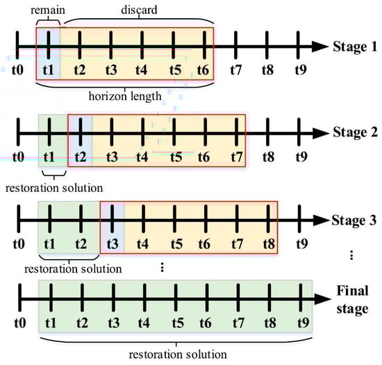
Figure 4.
The rolling-horizon-based technique proposed in [27].
Moreover, multi-stage approaches provide a systematic and structured methodology for tackling complex problems. In a multistage approach, instead of attempting to solve the problem all at once, the problem is divided into smaller, manageable stages, each addressing a specific aspect or subproblem. In [31], a two-stage scenario-based stochastic optimization was proposed for dispatching mobile emergency generators (MEGs) as DGs in the system to restore critical loads by forming multiple microgrids. Both of the stages were modeled as MILP problems. In the first stage, which is done before the blackout, a prepositioning of the MEGs is conducted to find the best place for the resources in the system. In the second stage, which is implemented after the disaster strikes, the real-time allocation of the MEGs is optimized. MEGs are dispatched from the locations determined in the first stage to the assigned locations to restore the loads. Since the MEGs need to travel on road networks, a vehicle-routing (VR) problem based on the Dijkstra’s shortest-path algorithm [54] was implemented in [31].
In addition, a two-stage framework was also proposed in [10] to first ensure restoration of the critical loads and then maintain a high survivability in extreme events. In this regard, the first stage determines the microgrid’s topology and resource allocation using a MILP formulation. In the second stage, the reconfiguration of the microgrids, considering repositioning the MEGs and shrinking the microgrids, is conducted based on a MILP method to minimize the loss of critical loads when the system encounters different outage scenarios in the extended event. The output of the first stage, i.e., system topology, is fed to the second stage to find the final optimal solution to the restoration problem. It should be noted that the proposed method is not an iterative process, meaning that there is no data flow from the second stage to the first one, and, after running the second stage using the results of the first stage, the final solution is detected.
Reference [18] proposed a three-stage framework for the restoration problem. In the first stage, the minimum and maximum values of the aggregated load range for each load node are determined based on a linear programming (LP) formulation. The loads are considered to have a flexible demand based on the determined range. In the second stage, a MILP-based optimization is run to solve the sequential service-restoration problem. The load demands are determined in this stage. The target load demand is then distributed among the houses connected to each node in the third stage through home energy management. A stochastic dual dynamic programming (SDDP) algorithm was used to solve the third-stage optimization based on the method described in [55]. In [17], a three-stage method was proposed for the restoration problem considering the repair crew (RC) dispatch. In the first stage, the RC routing problem is formulated as a VR problem to minimize the distance between the depots and damaged components and rapidly repair the damaged parts of the system. The second stage is a MILP model of the restoration problem. In the third stage, the Monte Carlo method was used to generate different scenarios to account for the uncertainties in the system. Then, the restoration plan is implemented in each scenario, and the results are revised using a risk-averse IGDT technique [56].
In [25], a three-level hierarchical framework was proposed to maximize the restored loads in the system. In the first level, all the restoration trees, from microgrids to critical loads, were obtained using the shortest path problem with an LP formulation. Then, the feasibility of each tree was verified using the power-flow calculation. In the second level, the dispatch and scheduling of emergency power-supply vehicles (EPSs) was formulated as a vehicle-routing problem considering the impact of traffic problems on load interruption time. The Dijkstra’s algorithm [54] was used at this level to find the shortest path (fastest route) from an origin to a destination. After restoring all the critical loads in the system, the restoration of the noncritical loads was implemented in the third level.
Also, a hierarchical structure was proposed in [33] to coordinate distribution-system operator (DSO) and virtual power plant (VPP) for sequential service restoration. VPPs are entities for the effective management of DERs which also have black-start capability. Each VPP consists of a BESS, PV system, EV charging station, microturbine, demand-response loads, and fixed loads. The VPPs perform self-scheduling optimization and provide the available resources to the DSOs. A rolling-horizon-based approach, similar to the method utilized in [27] (see Figure 4), was used in [33] to solve the VPP scheduling model over a fixed horizon and the sequential service restoration to find the sequential switching actions based on the available flexibility bounds of VPPs.
3.1.2. Heuristic Approaches
In this subsection, the heuristic approaches proposed in the literature for centralized methods are reviewed. In these approaches, the restoration problem is formulated as a multistage mathematical programming problem, and a heuristic technique is proposed to solve the problem in an effective manner. In [7], a two-stage heuristic approach based on the restoration paths was developed for critical service restoration. In the first stage, all the feasible restoration paths for each microgrid are included in the strategy table. In the second stage, the strategy table is revised to include only the valid paths based on the updated information received from the postevent situation in the network. The paths in the strategy table are potential solutions for the restoration problem. Then, a linear integer problem was proposed to find the final restoration strategy from the strategy table.
In [9], a multistep framework was proposed for the critical service restoration based on intentional islanding, as depicted in Figure 5. Accordingly, it is checked at the first step whether intentional islanding is required to restore critical loads. If so, heuristic rules are proposed to restore network and DG connectivity to pick up the critical loads. If any violation of the operational constraints is observed, a network-reconfiguration method is implemented in the next step to find a feasible solution. In the end, a load-shedding approach is used to fix the observed violations in the system if the system reconfiguration fails to find a feasible solution.
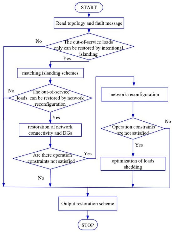
Figure 5.
The proposed multistep framework in [9].
In [23], a four-step procedure was proposed to find the best strategy for energizing the critical loads. The first step determines a unique path between each microgrid and critical load using the Dijkstra’s algorithm based on [57]. In the second step, load groups are formed for each tree, which are the set of critical loads that can be connected through a restoration tree. Then, the critical restoration problem was formulated as a maximum coverage problem and solved to find the restored loads in each load group and the corresponding restoration paths. The problem is a linear integer programming problem and can be solved using an off-the-shelf solver. In the last step, dynamic simulation of the network is utilized to find the restorative actions that need to be done to restore the loads. A greedy algorithm was used in this step to pick up the maximum number of loads at each step that should not violate any dynamic constraints.
Reference [22] proposed an iterative approach for the service-restoration problem considering the unbalanced operation of DGs. Accordingly, a penalty term proportional to the output power difference between each of the two phases of the DG is added to the objective function of the problem. Then, the problem is solved, and, if any violation in the output power of the DGs is observed, the weighting factor of the penalty term is increased (i.e., doubled in this paper) for the DG(s) for which a violation is observed. Then, the problem is solved with the new weighting factor. This process continues until no violation in the operation of the DGs is observed.
Also, in [6], a two-stage approach was proposed for critical load restoration coordinating multiple sources in the system, i.e., microgrids and DGs. In the first stage, the postrestoration topology is determined and the integer variables corresponding to the topological constraints are fixed in this stage. Then, the set of loads to pick up and output power of each source is defined in the second stage. This stage was formulated as a mixed-integer semidefinite program (MISDP) and relaxed to a semidefinite program by relaxing the integer variables (i.e., load status) as continuous variables. Then, an iterative algorithm was used to find the best integer value for each integer variable that was assigned a continuous value.
In [4], a look-ahead framework was proposed for load restoration in secondary networks. The approach is similar to the rolling-horizon-based method proposed in [27] (see Figure 4). The procedure to find the restoration plans consists of three steps. In the first step, a primary feeder with the maximum DG capacity that can supply the secondary system without any violation of the dynamic constraints is selected to serve the secondary loads. DGs on the selected primary feeder, along with the DGs in the secondary system, are used in an optimal generation schedule problem, which was formulated as a MILP, to find the optimal output power of the DGs and the loads to be restored in each time period. This step looks ahead from the current time step to the end of the restoration. Decisions made for the first period are kept, while the decisions for the rest of the time steps are disregarded. Based on the obtained results, the third step implements an operational dispatch to meet the power flow and operational constraints, which are based on a heuristic greedy approach. Also, the dynamic constraints are evaluated in this step, which may lead to load shedding due to maintaining the dynamic stability of the system.
3.2. Multiagent Methods
According to the combinatorial nature and complexity of the service-restoration problem, especially in large-scale practical networks, multiagent approaches can provide a decentralized or distributed framework, which facilitates distributed decision making across the system using multiple autonomous agents. This section reviews the multiagent approaches proposed for the black-start restoration, which are categorized into two main groups: mathematical programming and heuristic approaches.
3.2.1. Mathematical Programming
In this subsection, the systematic approaches proposed in the literature are reviewed, and different representations of agents are discussed. In [5,29,30,32], the authors proposed a multi-agent-based method for service restoration and formulated the problem as a MILP. They used off-the-shelf optimization solvers to find the optimal solution. Reference [5] proposed a distributed multiagent coordination approach using two types of agents: a local agent which has a limited computational capability, and a regional agent which is installed at DG nodes and equipped with an enhanced computation capability. An average consensus algorithm based on [58] was used in [5] to conduct the global information discovery. In [29], a virtual energization agent was proposed for each black-start DG, which can travel along energization paths and split into multiple agents, and energize the components. The problem is formulated as a routing problem and the solution to the routing problem is mapped to the service-restoration problem.
In [30,32], a synthetic routing model was proposed for a distribution-system restoration problem that integrates the crew-dispatch problem with the service restoration using three types of agents: an operation agent which is the crew for operating the manually operated switches, a repair agent which is the crew responsible for repairing any faulted component in the system, and an energization agent which is a grid-forming DG.
In [20], the authors proposed a fully distributed load-restoration model by exchanging limited information between the adjacent nodes and solving several small-scale subproblems. The alternating direction method of multipliers (ADMM) method was used to solve the decomposed model, which guarantees the convergence to an optimal solution of the relaxed problem in convex models. In this work, each node was modeled as an agent that only communicates with the adjacent nodes in the system.
3.2.2. Heuristic Approaches
Reference [8] proposed a heuristic rule-based approach to solve the decentralized multiagent service-restoration problem. Six different types of agents were considered in the proposed model, which represent different entities in the system, i.e., load agent, aggregator agent, dispatchable-DG agent, renewable-DG agent, battery energy storage (BES) agent, and switch agent. Each agent is allocated a specific task, which is manifested as a set of behaviors. These behaviors correspond to specific steps within the restoration strategy, indicating individual actions taken by each agent.
A deep reinforcement-learning-based algorithm was proposed in [34] for sequential service restoration. The problem is formulated as a Markov decision process (MDP) and is a deployed deep Q network (DQN) algorithm to solve the defined MDP. In this paper, each grid-forming DG is considered as an energization agent, as proposed in [29]. However, the agents can only take one action (i.e., switching action) at each time step and cannot enter a node that is already energized. An attention-mechanism-based method was used to model the coordination among the agents.
4. Test Systems and Tools
This section provides an overview of the various test systems and tools utilized in the black-start service-restoration methods. In Table 2, the different test systems which were deployed in the literature are summarized. The IEEE Test feeders and EPRI test cases are the most widely utilized in the literature. The data and different formats of the systems can be found on this website [59]. It should be noted that these test systems usually serve as a baseline network, and the researchers make their desired changes in the system to implement their proposed methods. Moreover, the simulation tools and optimization solvers utilized in the literature are summarized in Table 3. It should be noted that some studies did not explicitly mention the software and tools utilized in their work [8,36].
Table 2.
Summary of the test systems utilized in the literature.
Table 3.
Summary of the tools and software utilized in the literature.
5. Conclusions and Future Research Areas
This paper provides a comprehensive review of the existing journal papers that were published from 2016–2022 on black-start service-restoration methods in ADNs and MGs. The mathematical formulations of the problem and its various components in the literature are thoroughly discussed, followed by an overview of different implementation approaches proposed in the literature, such as centralized methods, multiagent approaches, and distributed approaches. This section highlights three key research areas that necessitate further exploration to formulate more effective solutions. These areas are based on the inherent characteristics of the black-start restoration problem. Accordingly, the distinctive aspects of the black-start restoration problem are discussed first, which offers valuable insights into the specific considerations that require careful attention and resolution in addressing the problem.
Black-start service restoration refers to the procedure of restoring ADNs that have been entirely de-energized due to a massive blackout or system collapse. The black-start restoration problem is characterized by a set of unique challenges. First and foremost, it places an extraordinary emphasis on system stability. The process must not only re-establish the power supply but also ensure that the power grid remains stable and does not fail during and after the restoration procedure while the system undergoes severe disturbances, such as the energization of big loads. Moreover, the initial states of the loads and generating units during the restoration are unknown, which significantly complicates the task of accurately forecasting both demand and generation levels. Additionally, during the restoration procedure, the behavior of loads becomes notably more unpredictable, given their response to the unique circumstances of a system-wide blackout. In addition, one of the remarkable attributes of black-start restoration is its interdependence with other critical infrastructures, such as communication networks and transportation systems. The effectiveness of restoration efforts depends on the availability and reliability of transportation systems, communication networks, fuel supplies, and security measures. Also, in the event of a large-scale blackout, resources such as personnel, equipment, and backup power sources may need to be shared between critical infrastructure sectors. Hence, collaborative resource sharing is a critical aspect of black-start restoration and relies on effective interdependence among the systems.
While significant progress has been made in the field of black-start service restoration, there are several research problems whose solutions hold the potential to further advance this field. In the following subsections, we highlight the abovementioned challenges that can contribute to the development of effective and more practical black-start restoration methods considering the practical and realistic modeling of the system behavior.
5.1. Dynamic Modeling of DGs and System Stability
During black-start restoration, the power system undergoes significant changes in operating conditions, including the switching of generators and the energization of loads. These changes can introduce transient disturbances and perturbations that can potentially lead to instability if not properly managed. Moreover, the absence of inertia in inverter-based DGs, which plays a key role in supplying the loads during the restoration, poses significant stability challenges during black-start restoration and dynamic operation of the power system. Inertia plays a critical role in maintaining frequency stability, damping oscillations, and supporting grid stability. Without sufficient inertia, the power system becomes more susceptible to frequency deviations and disturbances, leading to instability and potential disruptions. Accordingly, considering the dynamic operation of the DGs, especially the ones that provide a reference for voltage and/or frequency in the system, allows for a comprehensive understanding of their response to various disturbances and grid conditions and ensure a secure and robust restoration plan. However, most of the proposed methods in the literature have assumed an average model for the DGs by assuming dispatchable active and reactive power outputs. However, the voltage source inverter (VSI) control model should be used for the grid-forming DGs that can emulate the behavior of a synchronous machine by controlling the voltage and frequency in the ac system [60].
During the islanded operation of an MG, the VSI control mode of the grid-forming units is responsible for generation–consumption balance and frequency control in the system. In addition, a voltage regulation strategy is required to prevent voltage and/or reactive power oscillations [61]. This working principle of a VSI provides primary voltage and frequency regulation in islanded MGs. Accordingly, two main control strategies can be considered for MG island operation: single-master operation (SMO) and multimaster operation (MMO) [60]. In an SMO, a VSI is used as the voltage and frequency reference while all the other inverters operate in PQ mode. On the other hand, in an MMO, several inverters are operating in VSI mode with predefined frequency/active power and voltage/reactive power characteristics, and other PQ-controlled inverters may also exist in the system.
The inherent imbalance present in distribution systems represents a substantial challenge to their dynamic modeling and control, demanding efficient methods for dynamic and stability analysis. The most widely used method for dynamic modeling and stability analysis is based on the dq0 transformation. However, this approach is suitable exclusively in instances where the network maintains a balanced and symmetric configuration [62]. Another popular modeling technique is dynamic phasors, which extends the concept of quasistatic phasors. Dynamic phasors express voltage and current signals through Fourier series expansions, with harmonic components assessed over a moving time window [63]. Moreover, this approach can be effectively used in unbalanced networks. The idea behind the dynamic phasors approach is therefore to approximate the system with nearly periodic quantities, which allow an accurate representation of the system while using a relatively large numerical step size. A comparison of simulation techniques based on dynamic phasors in the abc and dq0 reference frames may be found in [64].
Addressing the dynamic behavior of DGs and ensuring stable and secure transient operation of the system during black-start restoration is a critical area that requires further exploration. While DGs offer significant potential for improving the restoration process, the specific challenges related to their dynamic behavior and system stability, especially for unbalanced distribution networks, need to be thoroughly investigated to develop feasible and practical solutions. Further studies are needed to investigate the impact of DGs on system dynamics, identify potential stability risks, and design control methods to mitigate those risks.
5.2. Uncertainty of Forecasted Load Demand and DG Generation
Extreme events often result in widespread outages and infrastructure damage throughout the system, making it challenging to accurately predict the postdisaster load demand and available generation capacity. Hence, in the context of black-start restoration following a natural disaster, uncertainties can emerge that surpass the typical uncertainty levels experienced during normal grid operations. These uncertainties are influenced by factors such as the presence of damaged or inaccessible infrastructure and changes in customer behavior in the aftermath of an extended outage. Accordingly, new techniques are required in this regard to address these uncertainties by gaining a comprehensive understanding of the sources of the uncertainties.
By accounting for load demand and generation uncertainties, restoration plans can be tailored to adapt to dynamic and unpredictable conditions, thereby facilitating effective resource allocation and coordination. Some studies in the literature addressed the uncertainties using well-known techniques. For example, in [21], a robust method based on the information-gap decision theory (IGDT) was utilized which models the uncertainties by uncertainty sets without requiring the probability distribution. However, the existing methods have not adequately accounted for the aforementioned new sources of uncertainties that arise in the black-start restoration. These uncertainties introduce additional complexities that can significantly impact the effectiveness of restoration plans. Failure to consider these uncertainties may lead to suboptimal decision making, inefficient resource allocation, and delays in restoring power to affected areas. Therefore, there is a need for further research and development of methods that explicitly address and incorporate these new sources of uncertainties in the black-start restoration process.
5.3. Interdependence with Other Infrastructure
Power systems are intricately linked with various critical infrastructures, such as transportation, water supply, communication, and gas systems. During the black-start procedure, the successful restoration of power relies not only on bringing the power grid back online but also on a comprehensive understanding of the interdependencies between these infrastructures. Failure to consider this interdependence can hinder the effectiveness of the overall restoration process and delay the resumption of essential services, prolonging the restoration time of the loads. The consideration of interdependence with other infrastructure in the context of black-start service restoration is still in its early stages. There are a few papers that considered power-system interdependence with transportation systems [24], communication systems [32], and natural gas systems [17] by explicitly modeling the systems in the restoration problem. The transportation system plays a critical role in supporting the restoration process by facilitating the mobilization of repair crews, equipment, and essential resources to the affected areas. Repair crews and technicians need to navigate affected areas to identify and address specific points of failure, damaged distribution lines, or malfunctioning equipment. This on-site assessment is critical for developing targeted restoration plans and prioritizing repair activities [19,24,30]. The transportation system enables the fast movement of personnel to affected sites, enabling a more accurate understanding of the extent of damage and facilitating efficient decision making. Furthermore, the transportation system plays a significant role in ensuring the timely delivery of essential resources and supplies during the restoration process. This includes the transportation of fuel for backup generators, replacement equipment, spare parts, and materials required for repairs. Also, the electrification of transportation, particularly through the adoption of EVs and fleets, can significantly tighten the interdependence between power systems and transportation networks.
On the other hand, effective communication infrastructure is essential for coordinating and managing restoration efforts, facilitating real-time monitoring, and enabling efficient decision making during black-start procedures. Communication systems play a vital role in maintaining situational awareness and coordination among various entities involved in the restoration process. Also, natural gas systems hold significant importance in the context of black-start service restoration, as some of the available power generation in the system is fueled by natural gas. Therefore, a continuous and uninterrupted supply of natural gas is vital to ensure the operation of these generators and initiate the black-start service restoration.
The complex nature of interdependent systems, along with the limited understanding of the intricate dependencies between different infrastructures and their specific requirements, presents challenges in effectively incorporating interdependency considerations into black-start restoration plans. Each infrastructure sector has unique operational characteristics, interconnections, and dependencies, making it challenging to develop comprehensive and tailored restoration strategies. Furthermore, the dynamic nature of interdependencies requires continuous monitoring, evaluation, and adaptation of restoration plans. As infrastructure systems evolve and become increasingly interconnected, new dependencies may emerge, necessitating ongoing analysis and adjustments to restoration strategies. Incorporating real-time data and advanced modeling techniques can facilitate a more accurate understanding of interdependencies and aid in the development of adaptive restoration solutions and plans that incorporate solutions involving multiple infrastructures.
Table 4 summarizes the discussed research gaps and provides a brief comparative analysis of the solutions proposed in the literature to address some aspects of the outlined research gaps.
Table 4.
Summarizing the solutions proposed in the literature to the outlined research gaps.
Author Contributions
A.H.-A. wrote the paper as a part of his PhD studies at Texas A&M University. K.L.B.-P. supervised the work. All authors have read and agreed to the published version of the manuscript.
Funding
This research received no external funding.
Data Availability Statement
No new data were created in this study. Data sharing is not applicable to this article.
Conflicts of Interest
The authors declare no conflicts of interest.
References
- Liang, X.; Saaklayen, M.A.; Igder, M.A.; Shawon, S.M.R.H.; Faried, S.O.; Janbakhsh, M. Planning and Service Restoration Through Microgrid Formation and Soft Open Points for Distribution Network Modernization: A Review. IEEE Trans. Ind. Appl. 2022, 58, 1843–1857. [Google Scholar] [CrossRef]
- Zidan, A.; Khairalla, M.; Abdrabou, A.M.; Khalifa, T.; Shaban, K.; Abdrabou, A.; Shatshat, R.E.; Gaouda, A.M. Fault Detection, Isolation, and Service Restoration in Distribution Systems: State-of-the-Art and Future Trends. IEEE Trans. Smart Grid 2017, 8, 2170–2185. [Google Scholar] [CrossRef]
- Panteli, M.; Mancarella, P. The Grid: Stronger, Bigger, Smarter?: Presenting a Conceptual Framework of Power System Resilience. IEEE Power Energy Mag. 2015, 13, 58–66. [Google Scholar] [CrossRef]
- Xu, Y.; Liu, C.-C.; Wang, Z.; Mo, K.; Schneider, K.P.; Tuffner, F.K.; Ton, D.T. DGs for Service Restoration to Critical Loads in a Secondary Network. IEEE Trans. Smart Grid 2019, 10, 435–447. [Google Scholar] [CrossRef]
- Chen, C.; Wang, J.; Qiu, F.; Zhao, D. Resilient Distribution System by Microgrids Formation After Natural Disasters. IEEE Trans. Smart Grid 2016, 7, 958–966. [Google Scholar] [CrossRef]
- Wang, Y.; Xu, Y.; He, J.; Liu, C.-C.; Schneider, K.P.; Hong, M.; Ton, D.T. Coordinating Multiple Sources for Service Restoration to Enhance Resilience of Distribution Systems. IEEE Trans. Smart Grid 2019, 10, 5781–5793. [Google Scholar] [CrossRef]
- Gao, H.; Chen, Y.; Xu, Y.; Liu, C.-C. Resilience-Oriented Critical Load Restoration Using Microgrids in Distribution Systems. IEEE Trans. Smart Grid 2016, 7, 2837–2848. [Google Scholar] [CrossRef]
- Sharma, A.; Srinivasan, D.; Trivedi, A. A Decentralized Multi-Agent Approach for Service Restoration in Uncertain Environment. IEEE Trans. Smart Grid 2018, 9, 3394–3405. [Google Scholar] [CrossRef]
- Wang, F.; Chen, C.; Li, C.; Cao, Y.; Li, Y.; Zhou, B.; Dong, X. A Multi-Stage Restoration Method for Medium-Voltage Distribution System With DGs. IEEE Trans. Smart Grid 2017, 8, 2627–2636. [Google Scholar] [CrossRef]
- Che, L.; Shahidehpour, M. Adaptive Formation of Microgrids With Mobile Emergency Resources for Critical Service Restoration in Extreme Conditions. IEEE Trans. Power Syst. 2019, 34, 742–753. [Google Scholar] [CrossRef]
- Chen, B.; Chen, C.; Wang, J.; Butler-Purry, K.L. Multi-Time Step Service Restoration for Advanced Distribution Systems and Microgrids. IEEE Trans. Smart Grid 2018, 9, 6793–6805. [Google Scholar] [CrossRef]
- Bassey, O.; Butler-Purry, K.L. Islanded Microgrid Restoration Studies with Graph-Based Analysis. Energies 2022, 15, 6979. [Google Scholar] [CrossRef]
- Bassey, O.; Butler-Purry, K.L. Black start restoration of islanded droop-controlled microgrids. Energies 2020, 13, 5996. [Google Scholar] [CrossRef]
- Chen, B.; Chen, C.; Wang, J.; Butler-Purry, K.L. Sequential Service Restoration for Unbalanced Distribution Systems and Microgrids. IEEE Trans. Power Syst. 2018, 33, 1507–1520. [Google Scholar] [CrossRef]
- Ding, T.; Wang, Z.; Jia, W.; Chen, B.; Chen, C.; Shahidehpour, M. Multiperiod Distribution System Restoration With Routing Repair Crews, Mobile Electric Vehicles, and Soft-Open-Point Networked Microgrids. IEEE Trans. Smart Grid 2020, 11, 4795–4808. [Google Scholar] [CrossRef]
- Ding, T.; Wang, Z.; Qu, M.; Wang, Z.; Shahidehpour, M. A Sequential Black-Start Restoration Model for Resilient Active Distribution Networks. IEEE Trans. Power Syst. 2022, 37, 3133–3136. [Google Scholar] [CrossRef]
- Gazijahani, F.S.; Salehi, J.; Shafie-Khah, M. A Parallel Fast-Track Service Restoration Strategy Relying on Sectionalized Interdependent Power-Gas Distribution Systems. IEEE Trans. Ind. Inform. 2023, 19, 2273–2283. [Google Scholar] [CrossRef]
- Hafiz, F.; Chen, B.; Chen, C.; Rodrigo de Queiroz, A.; Husain, I. Utilising demand response for distribution service restoration to achieve grid resiliency against natural disasters. IET Gener. Transm. Distrib. 2019, 13, 2942–2950. [Google Scholar] [CrossRef]
- Lei, S.; Chen, C.; Li, Y.; Hou, Y. Resilient Disaster Recovery Logistics of Distribution Systems: Co-Optimize Service Restoration With Repair Crew and Mobile Power Source Dispatch. IEEE Trans. Smart Grid 2019, 10, 6187–6202. [Google Scholar] [CrossRef]
- Roofegari Nejad, R.; Sun, W. Distributed Load Restoration in Unbalanced Active Distribution Systems. IEEE Trans. Smart Grid 2019, 10, 5759–5769. [Google Scholar] [CrossRef]
- Song, M.; Nejad, R.R.; Sun, W. Robust Distribution System Load Restoration With Time-Dependent Cold Load Pickup. IEEE Trans. Power Syst. 2021, 36, 3204–3215. [Google Scholar] [CrossRef]
- Wang, Z.; Wang, J.; Chen, C. A Three-Phase Microgrid Restoration Model Considering Unbalanced Operation of Distributed Generation. IEEE Trans. Smart Grid 2018, 9, 3594–3604. [Google Scholar] [CrossRef]
- Xu, Y.; Liu, C.-C.; Schneider, K.P.; Tuffner, F.K.; Ton, D.T. Microgrids for Service Restoration to Critical Load in a Resilient Distribution System. IEEE Trans. Smart Grid 2018, 9, 426–437. [Google Scholar] [CrossRef]
- Xu, Y.; Wang, Y.; He, J.; Su, M.; Ni, P. Resilience-Oriented Distribution System Restoration Considering Mobile Emergency Resource Dispatch in Transportation System. IEEE Access 2019, 7, 73899–73912. [Google Scholar] [CrossRef]
- Yang, L.-J.; Zhao, Y.; Wang, C.; Gao, P.; Hao, J.-H. Resilience-Oriented Hierarchical Service Restoration in Distribution System Considering Microgrids. IEEE Access 2019, 7, 152729–152743. [Google Scholar] [CrossRef]
- Ye, Z.; Chen, C.; Chen, B.; Wu, K. Resilient Service Restoration for Unbalanced Distribution Systems With Distributed Energy Resources by Leveraging Mobile Generators. IEEE Trans. Ind. Inform. 2021, 17, 1386–1396. [Google Scholar] [CrossRef]
- Zhang, Q.; Ma, Z.; Zhu, Y.; Wang, Z. A Two-Level Simulation-Assisted Sequential Distribution System Restoration Model With Frequency Dynamics Constraints. IEEE Trans. Smart Grid 2021, 12, 3835–3846. [Google Scholar] [CrossRef]
- Bassey, O.; Butler-Purry, K.L.; Chen, B. Dynamic Modeling of Sequential Service Restoration in Islanded Single Master Microgrids. IEEE Trans. Power Syst. 2020, 35, 202–214. [Google Scholar] [CrossRef]
- Chen, B.; Ye, Z.; Chen, C.; Wang, J. Toward a MILP Modeling Framework for Distribution System Restoration. IEEE Trans. Power Syst. 2019, 34, 1749–1760. [Google Scholar] [CrossRef]
- Chen, B.; Ye, Z.; Chen, C.; Wang, J.; Ding, T.; Bie, Z. Toward a Synthetic Model for Distribution System Restoration and Crew Dispatch. IEEE Trans. Power Syst. 2019, 34, 2228–2239. [Google Scholar] [CrossRef]
- Lei, S.; Wang, J.; Chen, C.; Hou, Y. Mobile Emergency Generator Pre-Positioning and Real-Time Allocation for Resilient Response to Natural Disasters. IEEE Trans. Smart Grid 2016, 9, 2030–2041. [Google Scholar] [CrossRef]
- Liu, X.; Zhang, B.; Chen, B.; Aved, A.; Jin, D. Towards Optimal and Executable Distribution Grid Restoration Planning With a Fine-Grained Power-Communication Interdependency Model. IEEE Trans. Smart Grid 2022, 13, 1911–1922. [Google Scholar] [CrossRef]
- Mohy-ud-din, G.; Muttaqi, K.; Sutanto, D. A Hierarchical Service Restoration Framework for Unbalanced Active Distribution Networks Based on DSO and VPP Coordination. IEEE Trans. Ind. Appl. 2022, 58, 1756–1770. [Google Scholar] [CrossRef]
- Zhao, T.; Wang, J. Learning Sequential Distribution System Restoration via Graph-Reinforcement Learning. IEEE Trans. Power Syst. 2022, 37, 1601–1611. [Google Scholar] [CrossRef]
- Arif, A.; Wang, Z.; Wang, J.; Mather, B.; Bashualdo, H.; Zhao, D. Load Modeling—A Review. IEEE Trans. Smart Grid 2018, 9, 5986–5999. [Google Scholar] [CrossRef]
- Xu, Y.; Liu, C.-C.; Schneider, K.P.; Ton, D.T. Placement of Remote-Controlled Switches to Enhance Distribution System Restoration Capability. IEEE Trans. Power Syst. 2016, 31, 1139–1150. [Google Scholar] [CrossRef]
- Liu, W.; Lin, Z.; Wen, F.; Ledwich, G. A wide area monitoring system based load restoration method. IEEE Trans. Power Syst. 2013, 28, 2025–2034. [Google Scholar] [CrossRef]
- Schneider, K.P.; Sortomme, E.; Venkata, S.; Miller, M.T.; Ponder, L. Evaluating the magnitude and duration of cold load pick-up on residential distribution using multi-state load models. IEEE Trans. Power Syst. 2015, 31, 3765–3774. [Google Scholar] [CrossRef]
- Kumar, V.; Kumar, H.C.R.; Gupta, I.; Gupta, H.O. DG Integrated Approach for Service Restoration Under Cold Load Pickup. IEEE Trans. Power Deliv. 2010, 25, 398–406. [Google Scholar] [CrossRef]
- Mohy-ud-din, G.; Muttaqi, K.M.; Sutanto, D. Transactive energy-based planning framework for VPPs in a co-optimised day-ahead and real-time energy market with ancillary services. IET Gener. Transm. Distrib. 2019, 13, 2024–2035. [Google Scholar] [CrossRef]
- Hafiz, F.; Queiroz, A.R.d.; Husain, I. Coordinated control of PEV and PV-based storage system under generation and load uncertainties. In Proceedings of the 2018 IEEE Industry Applications Society Annual Meeting (IAS), Portland, OR, USA, 23–27 September 2018; pp. 1–5. [Google Scholar]
- Chávez, H.; Baldick, R.; Sharma, S. Governor Rate-Constrained OPF for Primary Frequency Control Adequacy. IEEE Trans. Power Syst. 2014, 29, 1473–1480. [Google Scholar] [CrossRef]
- Baran, M.; Wu, F.F. Optimal sizing of capacitors placed on a radial distribution system. IEEE Trans. Power Deliv. 1989, 4, 735–743. [Google Scholar] [CrossRef]
- Baran, M.E.; Wu, F.F. Network reconfiguration in distribution systems for loss reduction and load balancing. IEEE Trans. Power Deliv. 1989, 4, 1401–1407. [Google Scholar] [CrossRef]
- Kersting, W.H. Distribution System Modeling and Analysis, 2nd ed.; Taylor & Francis: Abingdon, UK, 2006. [Google Scholar]
- Gan, L.; Low, S.H. Convex relaxations and linear approximation for optimal power flow in multiphase radial networks. In Proceedings of the 2014 Power Systems Computation Conference, Wroclaw, Poland, 18–22 August 2014; pp. 1–9. [Google Scholar]
- OpenDSS. EPRI Distribution System Simulator. Available online: http://sourceforge.net/projects/electricdss/ (accessed on 22 February 2016).
- Chassin, D.P.; Schneider, K.; Gerkensmeyer, C. GridLAB-D: An open-source power systems modeling and simulation environment. In Proceedings of the 2008 IEEE/PES Transmission and Distribution Conference and Exposition, Bogota, Columbia, 21–24 April 2008; pp. 1–5. [Google Scholar]
- Zimmerman, R.D.; Murillo-Sánchez, C.E.; Thomas, R.J. MATPOWER: Steady-State Operations, Planning, and Analysis Tools for Power Systems Research and Education. IEEE Trans. Power Syst. 2011, 26, 12–19. [Google Scholar] [CrossRef]
- Thurner, L.; Scheidler, A.; Schäfer, F.; Menke, J.H.; Dollichon, J.; Meier, F.; Meinecke, S.; Braun, M. Pandapower—An Open-Source Python Tool for Convenient Modeling, Analysis, and Optimization of Electric Power Systems. IEEE Trans. Power Syst. 2018, 33, 6510–6521. [Google Scholar] [CrossRef]
- Lavorato, M.; Franco, J.F.; Rider, M.J.; Romero, R. Imposing Radiality Constraints in Distribution System Optimization Problems. IEEE Trans. Power Syst. 2012, 27, 172–180. [Google Scholar] [CrossRef]
- Pang, K.; Wang, C.; Hatziargyriou, N.D.; Wen, F.; Xue, Y. Formulation of Radiality Constraintsfor Optimal Microgrid Formation. IEEE Trans. Power Syst. 2022, 38, 5341–5355. [Google Scholar] [CrossRef]
- Kumar, Y.; Das, B.; Sharma, J. Multiobjective, Multiconstraint Service Restoration of Electric Power Distribution System With Priority Customers. IEEE Trans. Power Deliv. 2008, 23, 261–270. [Google Scholar] [CrossRef]
- Dijkstra, E.W. A note on two problems in connexion with graphs. Numer. Math. 1959, 1, 269–271. [Google Scholar] [CrossRef]
- Hafiz, F.; Queiroz, A.R.d.; Husain, I. Multi-stage stochastic optimization for a PV-storage hybrid unit in a household. In Proceedings of the 2017 IEEE Industry Applications Society Annual Meeting, Cincinnati, OH, USA, 1–5 October 2017; pp. 1–7. [Google Scholar]
- Soroudi, A.; Amraee, T. Decision making under uncertainty in energy systems: State of the art. Renew. Sustain. Energy Rev. 2013, 28, 376–384. [Google Scholar] [CrossRef]
- Xu, Y.; Liu, C.C.; Schneider, K.P.; Ton, D.T. Toward a resilient distribution system. In Proceedings of the 2015 IEEE Power & Energy Society General Meeting, Denver, CO, USA, 26–30 July 2015; pp. 1–5. [Google Scholar]
- Olfati-Saber, R.; Fax, J.A.; Murray, R.M. Consensus and Cooperation in Networked Multi-Agent Systems. Proc. IEEE 2007, 95, 215–233. [Google Scholar] [CrossRef]
- IEEE PES Distribution Test Feeders. Available online: http://sites.ieee.org/pes-testfeeders/ (accessed on 28 May 2023).
- Lopes, J.A.P.; Moreira, C.L.; Madureira, A.G. Defining control strategies for MicroGrids islanded operation. IEEE Trans. Power Syst. 2006, 21, 916–924. [Google Scholar] [CrossRef]
- Lasseter, R.H.; Paigi, P. Microgrid: A conceptual solution. In Proceedings of the 2004 IEEE 35th Annual Power Electronics Specialists Conference (IEEE Cat. No.04CH37551), Aachen, Germany, 20–25 June 2004; Volume 4286, pp. 4285–4290. [Google Scholar]
- Belikov, J.; Levron, Y. Comparison of time-varying phasor and dq0 dynamic models for large transmission networks. Int. J. Electr. Power Energy Syst. 2017, 93, 65–74. [Google Scholar] [CrossRef]
- Stankovic, A.M.; Sanders, S.R.; Aydin, T. Dynamic phasors in modeling and analysis of unbalanced polyphase AC machines. IEEE Trans. Energy Convers. 2002, 17, 107–113. [Google Scholar] [CrossRef]
- Demiray, T.; Andersson, G. Comparison of the efficiency of dynamic phasor models derived from ABC and DQO reference frame in power system dynamic simulations. In Proceedings of the 7th IET International Conference on Advances in Power System Control, Operation and Management (APSCOM 2006), Hong Kong, China, 30 October–2 November 2006. [Google Scholar]

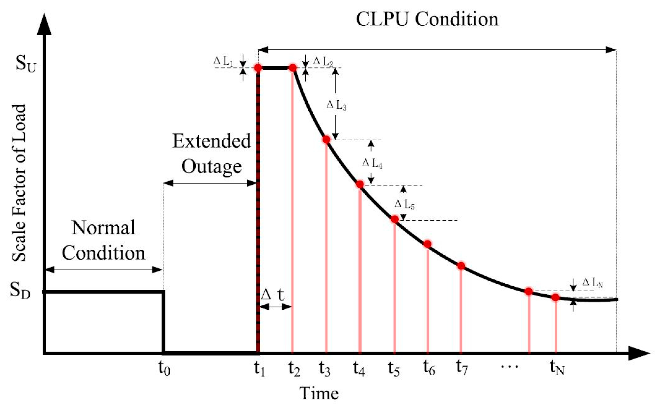
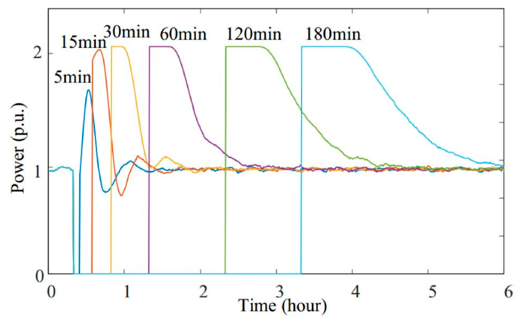
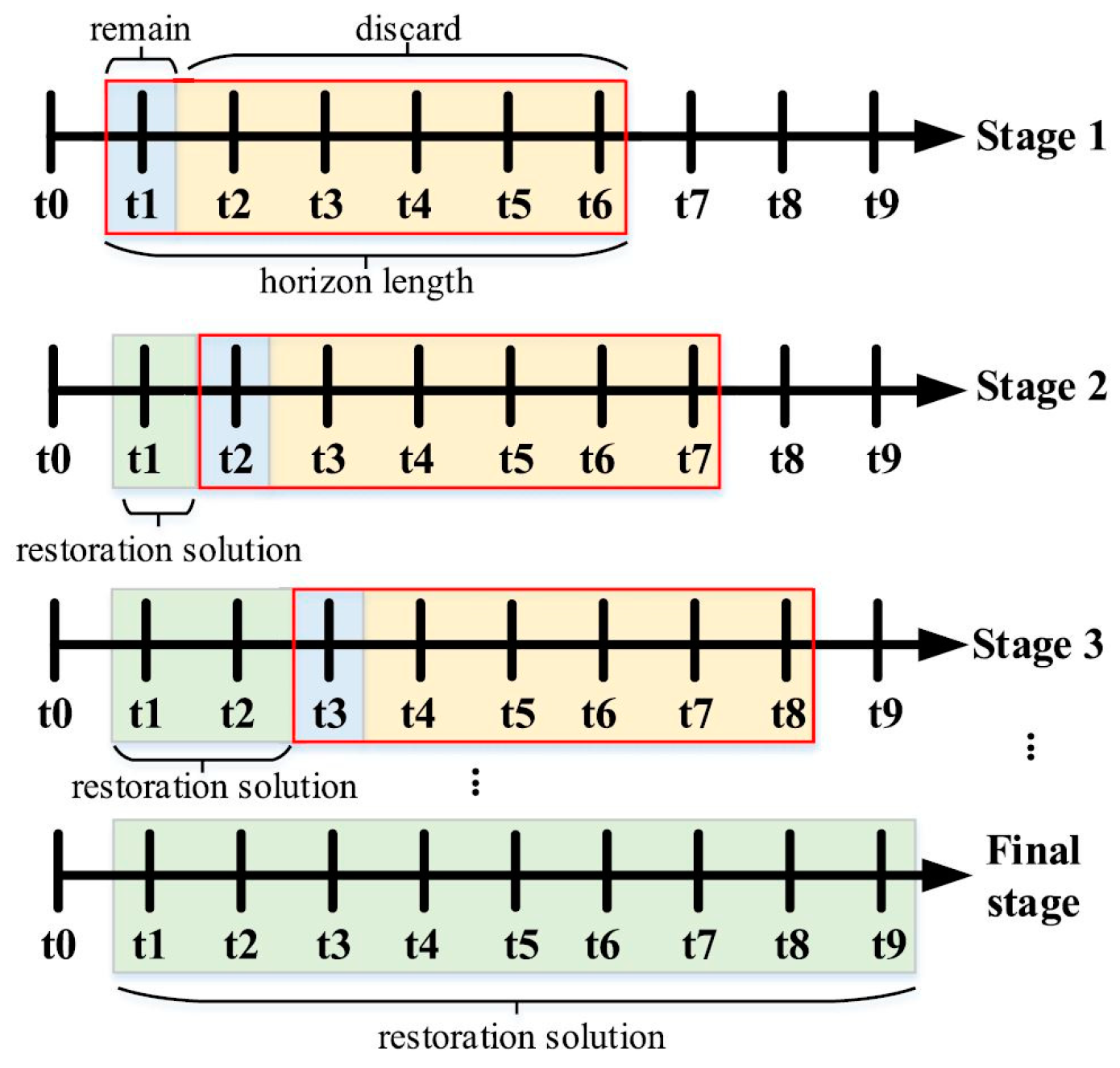

Disclaimer/Publisher’s Note: The statements, opinions and data contained in all publications are solely those of the individual author(s) and contributor(s) and not of MDPI and/or the editor(s). MDPI and/or the editor(s) disclaim responsibility for any injury to people or property resulting from any ideas, methods, instructions or products referred to in the content. |
© 2023 by the authors. Licensee MDPI, Basel, Switzerland. This article is an open access article distributed under the terms and conditions of the Creative Commons Attribution (CC BY) license (https://creativecommons.org/licenses/by/4.0/).