Article

A Generalised Series Model for the LES of Premixed and Non-Premixed Turbulent Combustion

by
Weilin Zeng
1,
Xujiang Wang
2,3,*,
Kai Hong Luo
4,*,
Konstantina Vogiatzaki
5 and
Salvador Navarro-Martinez
6
1
School of Mechanical Engineering, Chengdu University, Chengdu 610106, China
2
Shenzhen Research Institute of Shandong University, Shenzhen 518000, China
3
National Engineering Laboratory for Reducing Emissions from Coal Combustion, School of Energy and Power Engineering, Shandong University, Jinan 250061, China
4
Department of Mechanical Engineering, University College London, London WC1E 7JE, UK
5
Somerville College, Oxford University, Oxford OX1 2JD, UK
6
Department of Mechanical Engineering, Imperial College London, Exhibition Road, South Kensington, London SW7 2AZ, UK
*
Authors to whom correspondence should be addressed.
Energies 2024, 17(1), 252; https://doi.org/10.3390/en17010252
Submission received: 19 November 2023 / Revised: 13 December 2023 / Accepted: 14 December 2023 / Published: 3 January 2024
(This article belongs to the Section I2: Energy and Combustion Science)

Abstract

:
In this study, the generality and prediction accuracy of a generalised series model for the large eddy simulation of premixed and non-premixed turbulent combustion is explored. The model is based on the Taylor series expansion of the chemical source term in scalar space and implemented into OpenFOAM. The mathematical model does not depend on combustion regimes and has the correct limiting behaviour. The numerical error sources are also outlined and analysed. The model is first applied to a piloted methane/air non-premixed jet flame (Sandia Flame D). The statistical (time-averaged and RMS) results agree well with the experimental measurements, particularly with regard to the mixture fraction, velocity, temperature, and concentrations of major species CH4, CO2, H2O, and O2. However, the concentrations of the intermediates CO and H2 are over-predicted, due to the limitations of the reduced reaction mechanism employed. Then, a Bunsen-piloted flame is simulated. Most of the statistical properties of both the reactive species and progress variables are well reproduced. The only major discrepancy evident is in the temperature, which is probably attributed to the experimental uncertainties of temperature fields in the pilot stream. These findings demonstrate the model’s generality for both a premixed and non-premixed combustion simulation, as well as the accuracy of prediction of reactive species distribution.

1. Introduction

A challenge in the development of turbulent reacting models is the broad spectrum of the length and temporal scales introduced by large Reynolds (Re) and Damköhler (Da) numbers in modern combustors like advanced IC engines and gas turbines [1,2,3]. Compromising between the practicality of the Reynolds averaged Navier–Stokes (RANS) for industrial scale applications and the accuracy of direct numerical simulations (DNSs), the large eddy simulation (LES) has proven itself a promising technique for the simulation of propulsion and energy systems, if appropriate sub-grid-scale (SGS) models are employed. The vast majority of the established reactive SGS models are “borrowed” from those in RANS and can be classified into three categories [2,4]: (a) geometric approaches, such as flamelet [5], flame wrinkling [6], and thickened flame [7]; (b) statistical methods, including presumed [8] and transported probability distribution functions (PDF) [9] and conditional moment closures [10]/multiple mapping closures [11]; and (c) models based on turbulent mixing description, like eddy break up [12] and eddy dissipation assumption [13]. Extensive reviews can be found in [14,15,16].
While these models offer satisfactory predictions, if combined with fine grid resolutions, they rely heavily on assumptions related to specific combustion regimes or they are too expensive (such as the PDF transport model). Formerly, mathematical approaches based on series expansion were attempted within the RANS framework and were limited to conditions like supersonic combustion [17] and atmospheric boundary layers [2,18]. In RANS, the high-order series of the chemical source may partake larger contributions beyond the first-order one and may thus contribute nonnegligible truncation errors due to the substantial temporal oscillations of the temperature and species fraction. This gives rise to the challenging task of modelling accurately the involved scalar gradient ( Y F Y O ¯ , Y F T ¯ ). Nevertheless, the same challenge does not exist in LESs since filtering is operated in physical space (rather than the temporal averaging of RANS), so the higher-order contribution becomes less given a relatively well-resolved mesh and short time-stepping. This is evident in the research [19,20] on the LES of non-reactive flows in which a Taylor expansion on the filtered velocity field operates to close the SGS Reynolds stress in the Navier–Stokes equations. The simulation was validated against DNS and obtained satisfactory precision [21]. The model was later applied to modelling a neutral boundary layer flowing over a rough wall and the velocities coincided with theoretic solutions very well, ameliorating against standard eddy–viscosity approaches [19].
Similar mathematical methods [22,23] have also been proven feasible in the premixed turbulent combustion context, where series expansion is acted upon the reactive scalar field to determine the F factor in an artificially thickened flame (ATF) model. The LES of a turbulent Bunsen flame was conducted, and then accurate predictions regarding velocities and scalars were achieved [22,23]. For turbulent scalar signals, fourth-order terms were found not to play a major role [22].
Based on the above work, we have presented a novel series model for turbulent combustion in previous research [24]. The Taylor series expansion was performed in scalar space to avoid the highly spatial non-linearity of the chemical source term; meanwhile, the method was generalised for non-premixed and premixed combustion, owing to its mathematical derivation. This model was previously validated on premixed bluff-body stabilised flames [24]. Due to the experimental limitation of species information [25], we only briefly examined the predictive capability of combustion dynamics, velocity, and temperature profiles (but not species) in the premixed context, in addition to the grid resolution dependence [24].
In this paper, we build upon our previous work in order to provide a more detailed and well-rounded model evaluation. We extend the analysis of the model in the premixed regime with a new case (Bunsen jet flame F3 [26]) which benefits from a wider range of experimental data for validation. We also present the results for non-premixed cases (Sandia Flame D [27]) as the suitability of the model for non-premixed combustion has not been presented before. The objectives of this study are twofold: exploring the model’s generality for both premixed and non-premixed combustion simulation and assessing its prediction accuracy for reactive species distribution simulations. In the next sections, the derivation of the series model and the numerical implementation into OpenFOAM 2.4.0 is demonstrated, followed by the error analysis. Subsequently, the LESs of the two widely used validation benchmarks are presented. The results are analysed along with experimental data and data from previous relevant publications. Finally, the major conclusions and suggestions for future work are presented.

2. Methodology

2.1. Mathematical Formulation

The mathematical formulation is identical to that in the study [24]. In the LES governing equations [2], the SGS stress tensor is computed by the dynamic one equation eddy model [28], although other approaches can be, in principle, used. For the closure of reaction rates, a Taylor series expansion is operated in the scalar domain, averting the high nonlinearity in physical space (regarding the source term as a function of spatial coordinates). The chemical source term is first expanded in a single scalar form.
ω ˙ c = ω ˙ c - + ω ˙ c c = c - c x i δ x i + 1 2 2 ω ˙ c 2 c = c - c x i δ x i 2 +
Note that index notation is employed. Then, an isotropic filter is practiced to relation (1). All terms with odd powers of x, y, and z vanish by means of symmetry elimination [24]. For a detailed process, one can refer to the study [24] and the similar manipulations in the publications [19,20,21,22,23].
ω ˙ c ¯ = ω ˙ c - + Δ 2 24 2 ω ˙ c 2 c = c - c x i 2 ¯ + O ( Δ 4 )
The same processes are executed on the chemical source, a function of multiple scalars φ k , including chemical species, temperature, and pressure:
ω α ˙ φ 1 ,   φ 2 ,   , φ k ¯ = ω α ˙ φ 1 ¯ ,   φ 2 ¯ ,   , φ k ¯ + Δ 2 24 2 ω α ˙ φ 1 ,   φ 2 ,   , φ k φ m φ n φ 1 ,   φ 2 ,   , φ k = φ 1 ¯ ,   φ 2 ¯ ,   , φ k ¯ φ m x i φ n x i ¯ + O ( Δ 4 )
The unclosed scalar gradient term within, treated as the pseudo-scalar-dissipation form [2,17,18,24], is approximated by an algebraic expression approach [29]:
φ m x i φ n x i ¯ = φ m ¯ x i φ n ¯ x i + χ sgs   ( 1 + C s g s ) φ m ¯ x i φ n ¯ x i
For non-premixed combustion, C sgs is adopted as 0.1 following [30,31]. Otherwise, C sgs can be provided by transport equation models at the cost of high computational demands, which remains to be explored in the future.
Finally, the model turns out to be:
ω α ˙ φ 1 ,   φ 2 ,   , φ k ¯ = ω α ˙ φ 1 ¯ ,   φ 2 ¯ ,   , φ k ¯ + Δ 2 24 2 ω α ˙ φ 1 ,   φ 2 ,   , φ n φ m φ n φ 1 ,   φ 2 ,   , φ k = φ 1 ¯ ,   φ 2 ¯ ,   , φ k ¯ ( 1 +   C s g s ) φ m ¯ x i φ n ¯ x i + O Δ 4
The final closure in Expression (5) takes no presumption with respect to the combustion regime and, a priori, it is applicable for premixed, non-premixed, and partially premixed combustion. In addition, its accuracy is explicitly determined by the series truncation order. Finally, the approach preserves the reasonable restricting properties, where the SGS contribution decreases with the square of the filter width, see Relation (5), approaching DNSs as it reaches Kolmogorov scales. For more details, one can refer to the study [24].

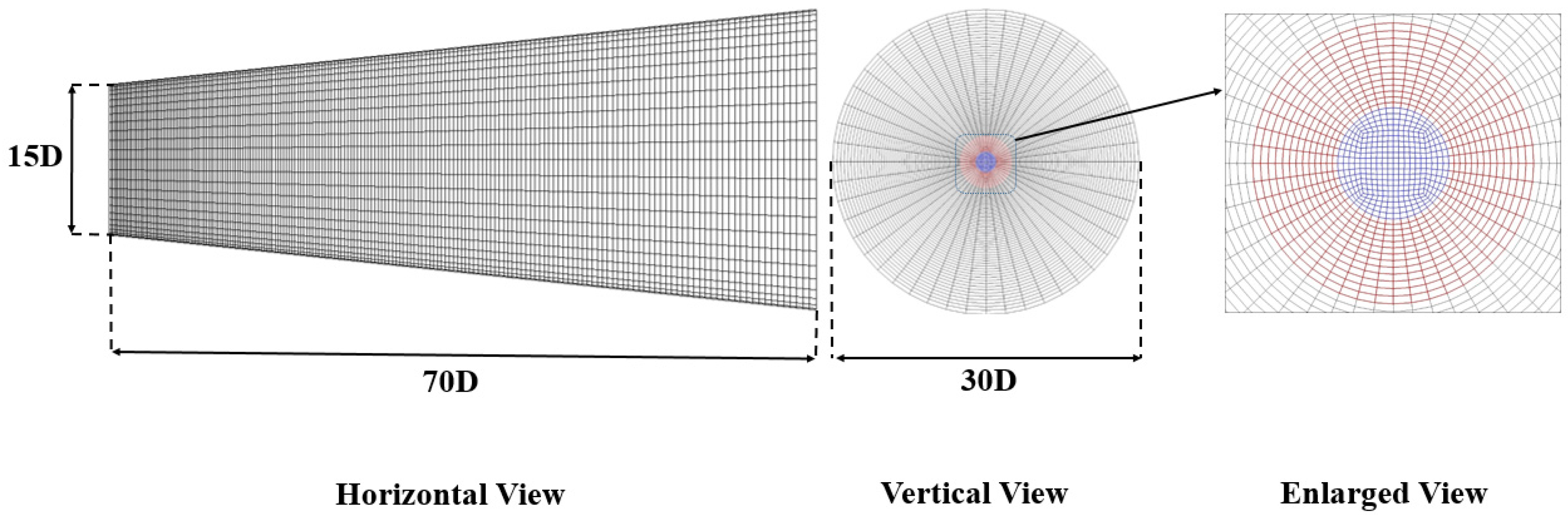
2.2. Numerical Implementation and Error Analysis

The series model is implemented on OpenFOAM platform [32]. In practice, the approach is incorporated in the reactingFoam solver through the manipulation of the chemical source in scalar balance equations. Additionally, the library combustionModel is customised to import the sub-grid part of the series model into the source term interface. In order to utilise the information of the Arrhenius reaction rate, the library chemicalModel is called. Then, the series model is coupled through the scalar transport equation with LES equations in the formation of a new reactingFoam-based solver. The PIMPLE algorithm is employed to deal with iterative procedures for the coupling equations of momentum and mass conservation.
Despite the series model being derived mathematically, computational errors inevitably will occur, like any other sub-grid combustion model. The sources of error can potentially stem from:
First, high-order terms. The accuracy of the model is mainly determined by the order of the Taylor series. In application, the terms of the fourth and higher order are neglected, as they have been discovered not to play a major role [23]. Nevertheless, under some extreme conditions, for example, in modelling deflagration and detonation transition, these higher-order contributions can significantly affect the flow field and lead to inaccuracy in predicting the sub-grid influence.
Second, the chemical mechanism. The series model requires the second derivative of the chemical source, which may become noisy under certain conditions. The choice of a well-established chemical scheme is crucial.
Thirdly, the scalar gradient term. The approximation in Equation (4) could be inaccurate in poorly resolved flames, where scalar gradients are large in the periphery of the reaction zones. This can be improved by employing a better refined/adaptive mesh.

3. Results and Discussion

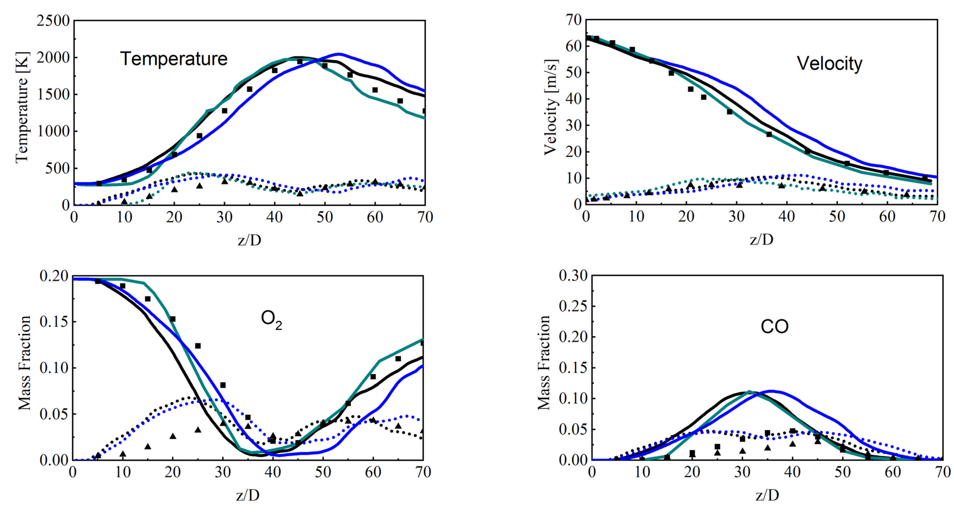
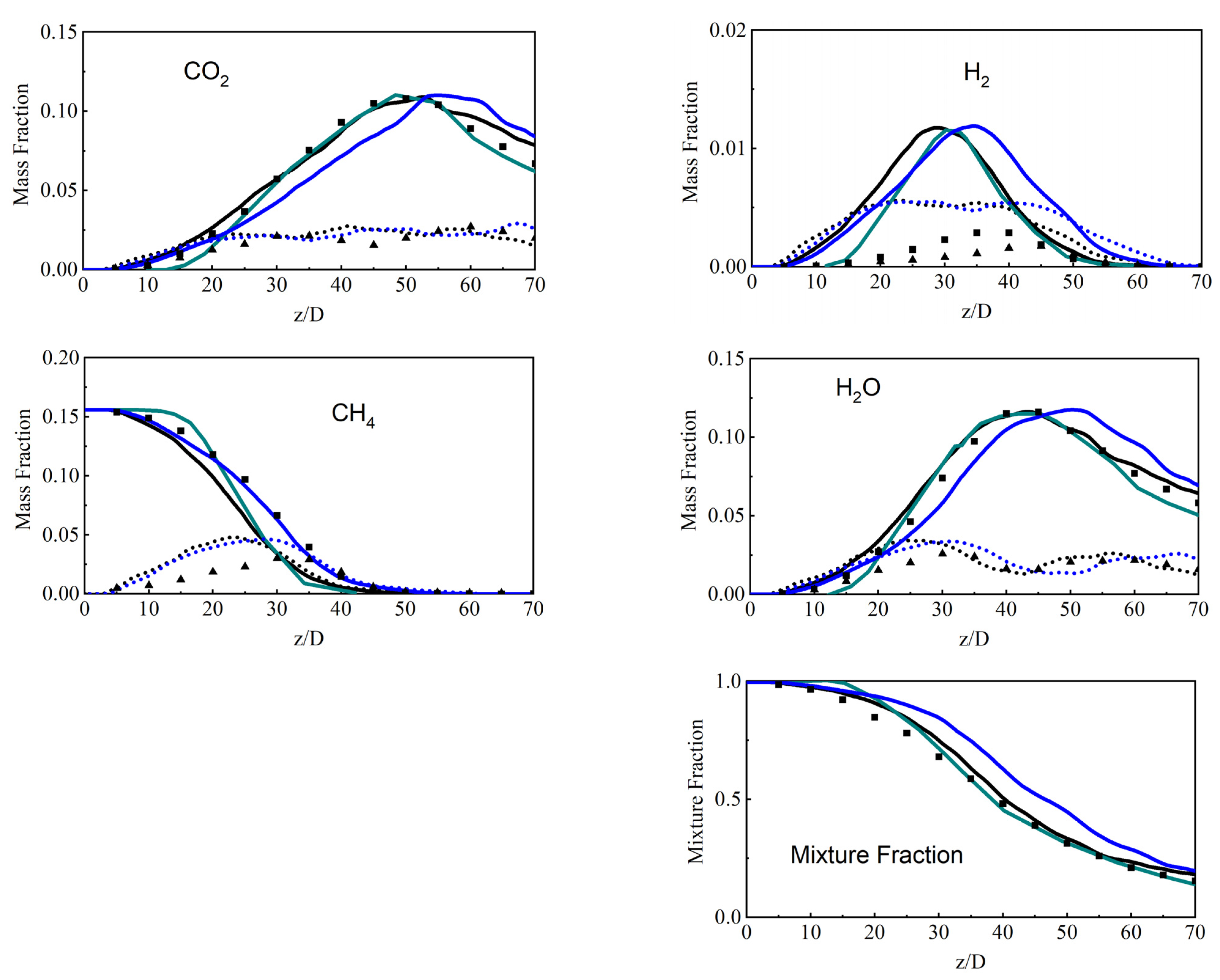
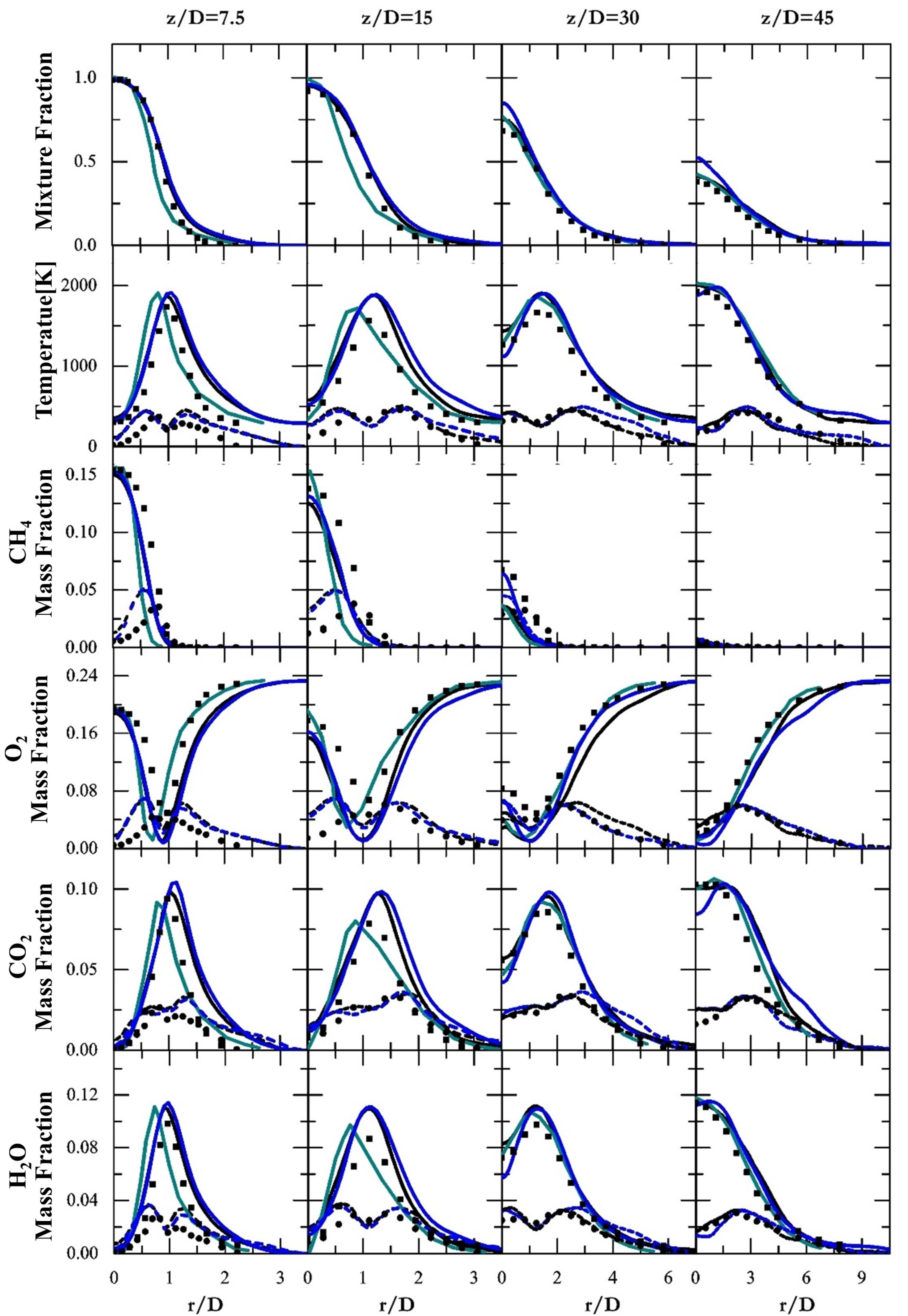
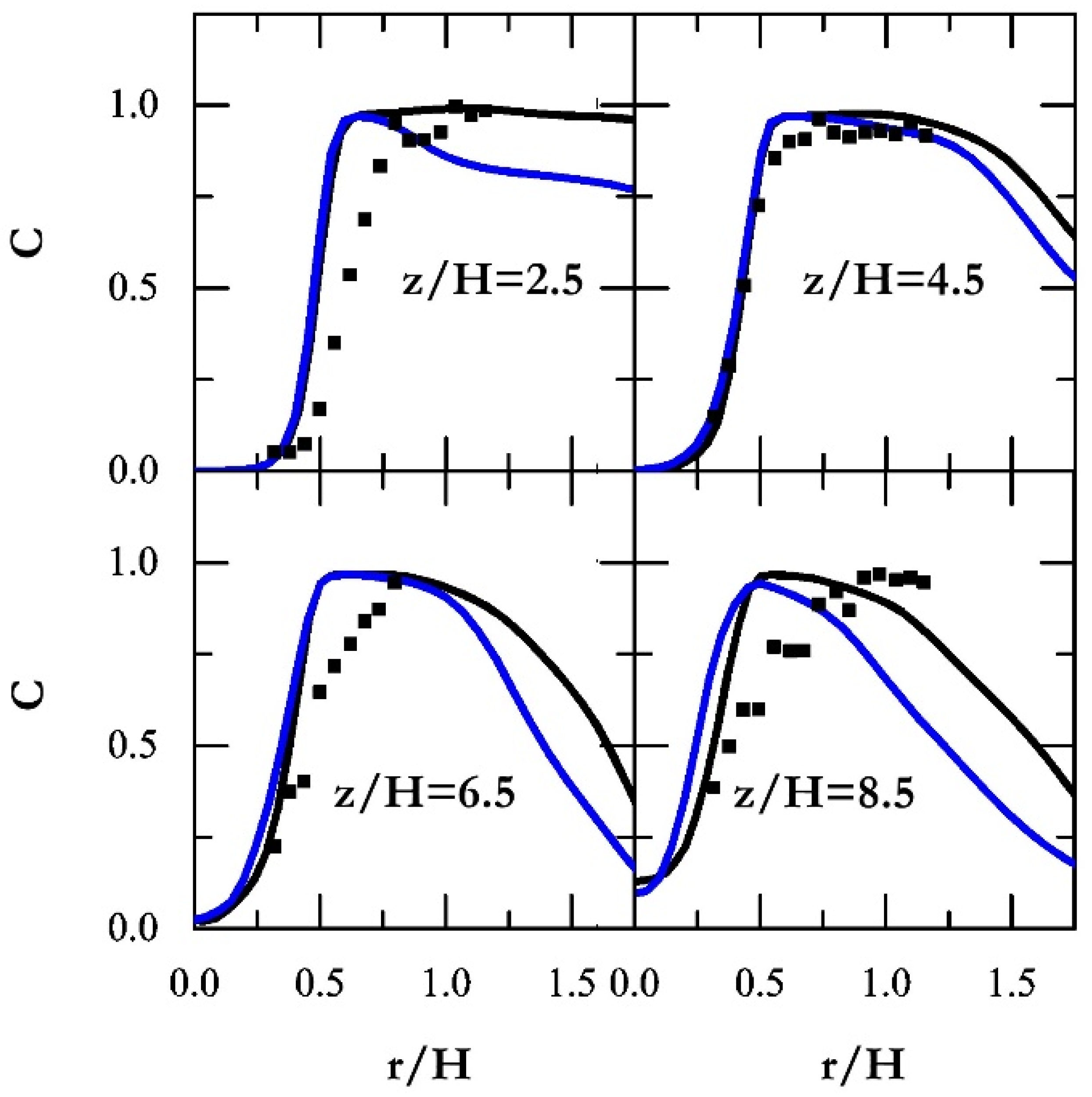
3.1. Non-Premixed Combustion Simulation

The case under consideration is Sandia Flame D, an ideal experimental benchmark for non-premixed combustion, broadly utilised for model verification in past studies due to the large set of experimental data available. Experimentally, this jet flame has been studied on a piloted burner at Sydney University [33] by Barlow [34], who measured the temperature and species field, and Schneider [27], who provided laser Doppler velocimetry (LDV) velocity details. The burner has an inner nozzle diameter D = 7.2 mm where a mixture of 25% methane and 75% air by volume is injected at a bulk velocity of 49.5 m/s, resulting in Re = 22,400. The pilot nozzle expands to a diameter of 18.2 mm, coaxial to the main jet. From it, exits a lean (Φ = 0.77, T = 1880 K) mixture of C2H2, H2, air, CO2, and N2 with the same nominal enthalpy and equilibrium composition as methane/air, at the same equivalence ratio, at a bulk velocity of 11.4 m/s. Surrounding the pilot nozzle, air streams at a velocity of 0.9 m/s. The burner exit is positioned approximately 15 cm above the exit of the vertical wind tunnel [34].
The details of modelling parameters are exhibited in Table 1, along with comparisons with previous studies. According to it, the radial domain widely chosen ranges from 8 to 40D in the radial direction, while the axial part ranges from 35 to 150D. In our work, the domain extends 70D in axial directions. Previous studies [35,36] suggested that clapping the grids to 50D does not affect the results, and in the radial direction, it has an increase from 15 to 30D to capture the downstream flame/temperature expansion. The sketch of the simulation domain and fine grid allocation is depicted in Figure 1. The mesh is aligned with polar coordinates, but in the centre, a square section (or o-grid, see the enlarged view in Figure 1) is applied to avoid very fine meshes in the centreline. Two resolutions are employed under the Pope criterion [37,38,39,40,41,42]: a fine grid of 71 points in the tangential direction, 48 points in the azimuthal direction, and 210 points in the axial direction, with an o-grid area of 12 × 12, and a coarse one, which is approximately downscaled with a factor of 1.5 in each direction (52, 36, and 139), with an o-grid zone of 9 × 9. Both grids stretch along the axial and tangential directions to handle the inlet variance and the strong gradients in shear layers.
Snapshots of the simulated instantaneous fully developed fields are shown in Figure 2. From the temperature and CO2 distribution, the predicted flame structure displays the conventional characteristics of non-premixed combustion [2] as expected: a preliminary area close to the inlet nozzle where flames are thin and a subsequent zone beside which hot products fill the majority of the downstream realm.
The statistical collection is performed over 16 burner flow-through times based on the jet bulk velocity. In addition, 10 flow-through times are initially computed to guarantee the flows are fully developed. To compare, published Flame D predictions by [43] in Table 1 are imported into the following result plots. The main reason is that it adopts the same four-step chemistry mechanism and uses the sophisticated Eulerian stochastic field method for combustion modelling. This allows us to evaluate the performance of the series method against a well-established and reliable model, avoiding the complexities associated with the chemical mechanism. The results (fine grid set) presented are carried with a similar resolution to the fine mesh employed in this study.
Figure 3 displays the mean and root-mean-square (RMS) trends of the mixture fraction, temperature, axial velocity, and species along the centreline, and Figure 4 shows the radial distributions. The mixture fraction is defined following Bilger [34]. Along the centreline, the series model shows good prediction with mixture fraction experimental data in the fine grid, with slight over-prediction from z/D = 10 to 40, illustrating that the flame shape is replicated reasonably. For the coarse resolution, the result shows a reasonable trend but diverges off the fine grid prediction from z/D = 15. This is largely due to the grid insufficiency of the coarse mesh in the downstream part. However, the situation is opposite in the reference case [43], where over-prediction is observed in the immediate vicinity of the inlet. The authors attributed this to the limited grid resolution of the mixing layers evolving between the jet and pilot close to the nozzle. Switching to the radial distributions in Figure 4, the mixture fraction profiles are well reproduced by the series model, although small over-predictions of the peak values are found at z/D = 30 and 45 in the coarse grid simulation. This is consistent with the centreline observations. The results from the stochastic fields method [43] are comparable in terms of accuracy with the series results, although some under-prediction in the inner (fuel-rich side) regions at z/D = 7.5 and 15 is noticed, which is not observed in the series model.
The axial profile of the mean and RMS temperature is also displayed in Figure 3. Along the centreline, the mean temperature and the flame location are well reproduced in the series model, and the fine grid prediction behaves better than the coarse one, as expected. The temperature RMS keeps the same level as the experimental data, although a small over-prediction appears in the upstream locations before z/D = 25. This evidences that the temperature fluctuation is sufficiently resolved by the series model with a simplified chemical mechanism. In addition, the RMS trend duplicates the observations in the experiments that the minimum arises around the location of the maximum mean profile. For the radial profiles in Figure 4, the statistical distributions agree well with the experiments, albeit with slight over-predictions of the mean values at z/D = 15 and 30. The over-predictions are also spotted in the reference case [43] and the discrepancies may originate from the thermal radiation that is not considered in both LES simulations. Furthermore, it should be noticed that the series model performs relatively better than the PDF method [43] at predicting the location of the mean peak at the near-nozzle positions z/D = 7.5 and 15. This is related to the under-prediction of mixture fraction profiles in the stochastic field simulation [43]. The centreline distribution of velocities is displayed in Figure 3 as well. Clearly, those quantities are decently reproduced by the series model, in spite of some acceleration after 15D in the coarse grid simulation. The stochastic field model [43] predicts a relatively better trend.
Figure 3 also exhibits the axial profiles of reactive species. Observing the series model results, the reactants CH4 and O2 tend to be consumed faster than the experimental data indicated, consistent with the slightly over-predicted temperature trend. The predictions of CO2 and H2O agree well with the measurements, though the coarse grid results are less accurate. Nevertheless, the prediction of CO and H2 is significantly over-predicted. The discrepancies as well as the accelerated CH4 decay rate are like those observed in the simulation [43] and can be attributed to the limitations of the simplified mechanism [42]. These findings [43,59] suggest that the C1 scheme in the mechanism [42] gives rise to an over-prediction of the reaction rates on the fuel-rich side of the non-premixed flames. This is evidenced in the radial distribution of CH4 in Figure 4. Additionally, the reduced reaction mechanism suffers from the shortcomings of predicting intermediates like H2 and CO as it is susceptible to diffusive transport [42]. This accounts for the inferior distributions of the same intermediate species in Figure 3. In spite of this, good radial agreement is achieved for both the series model and stochastic fields method [43], regarding the mean and RMS of CO2 and H2O. The peak locations near the nozzle exit are slightly under-predicted in the reference case [43], owing to the same reason of the temperature distribution.
Overall, both the mean and RMS behaviours of the non-premixed flame are well captured by the series model. Improvements are obtained with grid refinement, especially in terms of reproducing the temperature, mixture fraction, and major species distributions. In contrast to the stochastic field approach using the same mechanism [43], the series model demonstrates comparatively good prediction in general, and even better on some occasions, like correctly capturing the radial distributions of mixture fractions and the peak locations of mean temperature and chemical species. This gives the series model an advantage to some extent since its formulation is simpler, its cost cheaper, and it can be incorporated directly into the species transport equation.

3.2. Premixed Combustion Simulation

In this section, the methane/air turbulent Bunsen flame F3 experimented on by Chen [26] is chosen. The configuration is a typical turbulent premixed flame, with a wide range of available velocity, temperature, and species experimental data provided from [25], which has been extensively applied for model validation in the combustion community. The burner has an inner nozzle with a diameter H = 12 mm from which a stoichiometric mixture of methane and air is injected at different bulk velocities of 30 m/s, leading to Re = 23,000. Surrounding the main fuel injection, a laminar stream (the burning products of stoichiometric methane and air) is piloted via a perforated plate for stabilising the turbulent flame [60], and the outer diameter is 68 mm. Outward, the fresh air is entrained as a form of a low-velocity co-flow. In the diagram of the premixed regimes, the F3 flame lies in the thin reaction zone, more precisely, near the flamelet regime.
Simulation details are presented in Table 2, along with comparisons with previous research. The simulated domain extends 30H downstream of the nozzle and 12H in the radial direction so as to capture the downstream flame/temperature expansion. As Table 2 summarises, the chosen domain is sufficient for flame propagation. The grid used is aligned with polar coordinates, but in the centre, a square section (o-grid) is applied to avoid very fine meshes in the centreline as in Sandia Flame D. Two resolutions are employed following the Pope criterion [37]: a fine grid of 69 points in the tangential direction, 48 points in the azimuthal direction, and 200 nodes in the axial direction; and a coarse one, which is approximately downscaled with a factor of 1.5 in each direction (49, 36, and 134). Grids are stretched along the axial and tangential directions to seize the strong gradients stemming close to the nozzle and shear layers. The sketch of the simulation domain and grid allocation is detailed in Figure 5.
On the inlet boundary, velocity is prescribed with the detailed flow field experimental data [26] above the nozzle exit. The inlet turbulence intensities are imposed using the same approach as the Sandia D flame. For the main jet species, flat profiles are specified using the measurements from [26]. The composition of the pilot stream follows [60]. The pilot temperature is presumed as 1785 K [60,73,74], corresponding to 20% heat loss. Free slip is used for the lateral boundary, while a non-reflecting outflow condition is used on the outflow plane. The numerical schemes, the time set-up, and the chemistry mechanism are the same as in Sandia Flame D simulations.
The statistical collection is performed over 15 burner flow-through times based on the jet bulk velocity. Before it, eight flow-through times are computed to guarantee the flows are fully developed. As a comparison, a set of F3 flame predictions published by [22] in Table 2 is selected, since it adopts a similar mathematical approach based on the Taylor series expansion on the scalar field to determine the F factor in the ATF model. The augmented reduced version of GRI 3.0 schemes is introduced to denote chemistry. Furthermore, the mesh resolution is higher than the fine grid in this work.
The radial profiles of the mean temperature and reactive species at different streamwise locations are first depicted in Figure 6. Overall, the mean temperature is over-produced, especially near the nozzle. However, different researchers [60,64,66,67,69,75] reported the over-prediction discrepancies related to experimental measurements (largely extending 10–25% experimental uncertainties) using either reduced or detailed mechanisms. This discrepancy is largely due to the uncertainties of temperature fields in the pilot stream, where a large and unidentified portion (not reported in experiments [26]) of heat is lost to the burner exteriors [64,67]. The past studies listed in Table 2 indicate that the loss proportion varies between 0% and 34% [60,64,65,70]. On the other hand, the simulation domain starts just downstream of the nozzle exit for computational cost reduction, and wall heat transfer is not considered. For the experiment, the nozzle extends below the simulation domain, and heat loss to the wall could be the reason why the experimental measurements are lower than the simulation results.
The radial trends of species mass fraction are displayed in Figure 6. The profiles of CH4 and O2 are reasonably replicated; in spite of some minor under-predictions on the fuel-lean sides (r/H > 0.5), the calculated reactants meet the measurements well at the fuel-rich side and keep the descending trend from upstream to downstream. This indicates that the consummation rates of CH4 and O2 are well-reproduced along the centreline. In contrast, the reference results [22] are under-predicted on both the fuel-lean and fuel-rich sites.
The radial distributions of CO2 and H2O by the series model show a reasonably decent consistency with experimental observations, despite some under-predictions at z/H = 6.5. Meanwhile, improvements are obvious with the increase in grid resolutions. Compared with the reference case [22], the series model performs better on the fuel-rich sides. This is because the profiles of the reactants CH4 and O2 are not well resolved in these areas [22]. Note that in ATF models, although the thickened flames are solved, the species transport equation is modified and the interaction between combustion and turbulence is transformed from a transport-dominant combustion regime to a chemistry-dominant one, and the impact of the heat release upon the flow field is not represented sufficiently. In contrast, the series model operates on the reaction rate term directly, without altering the formation of the species balance equations. In terms of CO, the series model also obtains a good prediction, while the profiles are slightly under-predicted in the reference case [22]. On the other hand, the computed CO products are less sensitive to grid resolutions than major species, as less difference is found with grid refinement. The measurement error of major species varies from 8% to 15% and that of intermediate species reaches 25% [26]. The major and intermediate species predicted by the series model principally cater to the accuracy in both grid resolutions.
To further inspect the impact of the temperature discrepancies, a new progress variable is established by the definition of a linear combination of species concentration [76]:
c = Y C O 2 + Y C O ( Y C O 2 + Y C O ) p i l o t
The radial distribution is depicted in Figure 7 and compared with experimental measurements. In this regard, the progress variable based on species demonstrates a reasonable and much better agreement than the temperature profile. The trend is refined even in the vicinity of the nozzle exit where substantial discrepancies in the mean temperature are detected.
Usually, in non-premixed combustion where the flame is thick, one would eventually start resolving as the mesh is refined. However, in premixed combustion, the reaction zones are very thin and would always remain under the grid size in the LES. In general, with the refinement in grid resolution, the series model improves at predicting the premixed Bunsen flame. Comparing the series model with the simulations in [22], which adopted a similar series approach to determine the F factor of the artificially thickened flame model, the predictions are as good, if not better. Considering that the reference simulation [22] employs a finer mesh and more detailed chemistry, the series model shows the potential improvement when finer meshes or/and more detailed chemistry are used.

4. Conclusions

The generality and prediction accuracy of the series model for the LES of premixed and non-premixed turbulent combustion are presented. They are based on the Taylor series expansion of the chemical source term in scalar space around the filtered value and implemented into OpenFOAM. The mathematical model does not depend on specific combustion regimes, has the correct limiting behaviour, and determines the order of accuracy explicitly.
The model is first applied to a piloted methane/air non-premixed jet flame (Sandia Flame D) with two mesh resolutions. The statistical (time-averaged and RMS) results of the mixture fraction, velocity, temperature, and the concentrations of major reactive species CH4, CO2, H2O, and O2 are shown to be in reasonably well agreement with the experimental measurements. The discrepancies appear in the centreline and with the radial distribution of the intermediates CO and H2; this over-prediction is probably due to the limitations of the reduced reaction mechanism employed in the simulation. In contrast to the stochastic field approach using the same mechanism, the series model demonstrates comparatively good prediction in general, and is even better on some occasions, like when correctly capturing the radial distributions of mixture fractions and the peak locations of the mean temperature and chemical species.
Then, a Bunsen-piloted premixed flame was simulated. The statistical properties of the reactive species CH4, O2, CO2, H2O, and CO and progress variables are well reproduced by the series model. The major discrepancy lies in the temperature, which is attributed to the experimental uncertainties of the temperature fields in the pilot stream and the adiabatic boundary condition. Compared to the artificially thickened flame model that adopts a similar series approach to determine the F factor, the predictions are as good, if not better. Considering that the reference simulation employs a finer mesh and more detailed chemistry, the series model shows the potential improvement when finer meshes or/and more detailed chemistry are used.
Overall, the results demonstrated the model’s generality for both a premixed and non-premixed combustion simulation and its accuracy in the prediction of reactive species distribution. Future research will explore the applicability of partially premixed flames with detailed chemistry.

Author Contributions

Conceptualisation, K.H.L., K.V. and S.N.-M.; methodology, K.H.L., K.V. and W.Z.; software, W.Z. and K.V.; validation, W.Z. and K.V.; formal analysis, W.Z.; investigation, W.Z.; resources, K.H.L. and X.W.; data curation, W.Z.; writing—original draft preparation, W.Z.; writing—review and editing, K.H.L., K.V. and X.W.; visualisation, W.Z.; supervision, K.H.L.; project administration, K.H.L.; and funding acquisition, K.H.L. and X.W. All authors have read and agreed to the published version of the manuscript.

Funding

This work was supported by the Guangdong Basic and Applied Basic Research Foundation (Grant No. 2020A1515110720), China Postdoctoral Science Foundation (Grant No. 2020M682178), and Natural Science Foundation of Shandong Province (Grant No. ZR2021QE144).

Data Availability Statement

Data are contained within the article.

Conflicts of Interest

The authors declare no conflict of interest.

Nomenclature

c Species mass concentration α Chemical species
C s g s Sub-grid coefficient Δ Filter size
DSandia flame D inlet diameter φ k Field scalar
DaDamköhler number χ Scalar dissipation rate
hrsHours ω ˙ c Chemical source term
HBunsen flame F3 inlet diameterxjThe spatial vector
rRadial offsetYSpecies mass fraction
ReReynolds numberzThe spatial z-direction vector
TTemperature

References

  1. Taamallah, S.; Vogiatzaki, K.; Alzahrani, F.M.; Mokheimer, E.M.; Habib, M.; Ghoniem, A.F. Fuel flexibility, stability and emissions in premixed hydrogen-rich gas turbine combustion: Technology, fundamentals, and numerical simulations. Appl. Energy 2015, 154, 1020–1047. [Google Scholar] [CrossRef]
  2. Poinsot, T.; Veynante, D. Theoretical and Numerical Combustion; RT Edwards, Inc.: Morningside, Australia, 2005. [Google Scholar]
  3. Jiang, X.; Luo, K. Combustion-induced buoyancy effects of an axisymmetric reactive plume. Proc. Combust. Inst. 2000, 28, 1989–1995. [Google Scholar] [CrossRef]
  4. Giacomazzi, E.; Battaglia, V.; Bruno, C. The coupling of turbulence and chemistry in a premixed bluff-body flame as studied by LES. Combust. Flame 2004, 138, 320–335. [Google Scholar] [CrossRef]
  5. Popp, S.; Hunger, F.; Hartl, S.; Messig, D.; Coriton, B.; Frank, J.H.; Fuest, F.; Hasse, C. LES flamelet-progress variable modeling and measurements of a turbulent partially-premixed dimethyl ether jet flame. Combust. Flame 2015, 162, 3016–3029. [Google Scholar] [CrossRef]
  6. Volpiani, P.S.; Schmitt, T.; Vermorel, O.; Quillatre, P.; Veynante, D. Large eddy simulation of explosion deflagrating flames using a dynamic wrinkling formulation. Combust. Flame 2017, 186, 17–31. [Google Scholar] [CrossRef]
  7. Filho, F.L.S.; Kuenne, G.; Chrigui, M.; Sadiki, A.; Janicka, J. A consistent Artificially Thickened Flame approach for spray combustion using LES and the FGM chemistry reduction method: Validation in Lean Partially Pre-vaporized flames. Combust. Flame 2017, 184, 68–89. [Google Scholar] [CrossRef]
  8. Malalasekera, W.; Ranga-Dinesh, K.; Ibrahim, S.S.; Masri, A.R. LES of recirculation and vortex breakdown in swirling flames. Combust. Sci. Technol. 2008, 180, 809–832. [Google Scholar] [CrossRef]
  9. Gallot-Lavallée, S.; Jones, W.; Marquis, A. Large Eddy Simulation of an ethanol spray flame under MILD combustion with the stochastic fields method. Proc. Combust. Inst. 2017, 36, 2577–2584. [Google Scholar] [CrossRef]
  10. Navarro-Martinez, S.; Kronenburg, A. Flame stabilization mechanisms in lifted flames. Flow Turbul. Combust. 2011, 87, 377–406. [Google Scholar] [CrossRef]
  11. Farrace, D.; Chung, K.; Pandurangi, S.S.; Wright, Y.M.; Boulouchos, K.; Swaminathan, N. Unstructured LES-CMC modelling of turbulent premixed bluff body flames close to blow-off. Proc. Combust. Inst. 2017, 36, 1977–1985. [Google Scholar] [CrossRef]
  12. Spalding, D.B. Development of the eddy-break-up model of turbulent combustion. Symp. (Int.) Combust. 1977, 16, 1657–1663. [Google Scholar] [CrossRef]
  13. Ertesvåg, I.S.; Magnussen, B.F. The eddy dissipation turbulence energy cascade model. Combust. Sci. Technol. 2000, 159, 213–235. [Google Scholar] [CrossRef]
  14. Gicquel, L.Y.; Staffelbach, G.; Poinsot, T. Large eddy simulations of gaseous flames in gas turbine combustion chambers. Prog. Energy Combust. Sci. 2012, 38, 782–817. [Google Scholar] [CrossRef]
  15. Pitsch, H. Large-eddy simulation of turbulent combustion. Annu. Rev. Fluid Mech. 2006, 38, 453–482. [Google Scholar] [CrossRef]
  16. Janicka, J.; Sadiki, A. Large eddy simulation of turbulent combustion systems. Proc. Combust. Inst. 2005, 30, 537–547. [Google Scholar] [CrossRef]
  17. Villasenor, R.; Chen, J.-Y.; Pitz, R. Modeling ideally expanded supersonic turbulent jet flows with nonpremixed H2-air combustion. AIAA J. 1992, 30, 395–402. [Google Scholar] [CrossRef]
  18. Nieuwstadt, F.; Meeder, J. Large-eddy simulation of air pollution dispersion: A review. In New Tools in Turbulence Modelling; Springer: Berlin/Heidelberg, Germany, 1997; pp. 265–280. [Google Scholar]
  19. Chow, F.K.; Street, R.L.; Xue, M.; Ferziger, J.H. Explicit filtering and reconstruction turbulence modeling for large-eddy simulation of neutral boundary layer flow. J. Atmos. Sci. 2005, 62, 2058–2077. [Google Scholar] [CrossRef]
  20. Katopodes, F.V.; Street, R.; Ferziger, J. Subfilter-scale scalar transport for large-eddy simulation. In Proceedings of the 14th Symposium on Boundary Layers and Turbulence, Aspen, CO, USA, 12 August 2000; American Meteorologic Society Aspen (CO): Boston, MA, USA, 2000; pp. 472–475. Available online: https://ams.confex.com/ams/AugAspen/techprogram/paper_14491.htm (accessed on 18 November 2023).
  21. Katopodes, F.V.; Street, R.L.; Ferziger, J.H. A Theory for the Subfilter-Scale Model in Large-Eddy Simulation. Environmental Fluid Mechanics Laboratory Tech. Rep. (2000) K1. Available online: https://ui.adsabs.harvard.edu/abs/2001APS..DFD.AE005K/abstract (accessed on 18 November 2023).
  22. Domingo, P.; Vervisch, L. Large Eddy Simulation of premixed turbulent combustion using approximate deconvolution and explicit flame filtering. Proc. Combust. Inst. 2015, 35, 1349–1357. [Google Scholar] [CrossRef]
  23. Domingo, P.; Vervisch, L. DNS and approximate deconvolution as a tool to analyse one-dimensional filtered flame sub-grid scale modelling. Combust. Flame 2017, 177, 109–122. [Google Scholar] [CrossRef]
  24. Zeng, W.; Vogiatzaki, K.; Navarro-Martinez, S.; Luo, K.H. Modelling of Sub-Grid Scale Reaction Rate Based on a Novel Series Model: Application to a Premixed Bluff-Body Stabilised Flame. Combust. Sci. Technol. 2019, 191, 1043–1058. [Google Scholar] [CrossRef]
  25. Sjunnesson, A.; Nelsson, C.; Max, E. LDA measurements of velocities and turbulence in a bluff body stabilized flame. Laser Anemometry 1991, 3, 83–90. [Google Scholar]
  26. Chen, Y.-C.; Peters, N.; Schneemann, G.; Wruck, N.; Renz, U.; Mansour, M.S. The detailed flame structure of highly stretched turbulent premixed methane-air flames. Combust. Flame 1996, 107, 223-IN2. [Google Scholar] [CrossRef]
  27. Schneider, C.; Dreizler, A.; Janicka, J.; Hassel, E. Flow field measurements of stable and locally extinguishing hydrocarbon-fuelled jet flames. Combust. Flame 2003, 135, 185–190. [Google Scholar] [CrossRef]
  28. Fureby, C.; Tabor, G.; Weller, H.; Gosman, A. A comparative study of subgrid scale models in homogeneous isotropic turbulence. Phys. Fluids 1997, 9, 1416–1429. [Google Scholar] [CrossRef]
  29. Knudsen, E.; Richardson, E.; Doran, E.; Pitsch, H.; Chen, J. Modeling scalar dissipation and scalar variance in large eddy simulation: Algebraic and transport equation closures. Phys. Fluids 2012, 24, 055103. [Google Scholar] [CrossRef]
  30. Navarro-Martinez, S.; Kronenburg, A. LES-CMC simulations of a turbulent bluff-body flame. Proc. Combust. Inst. 2007, 31, 1721–1728. [Google Scholar] [CrossRef]
  31. Branley, N.; Jones, W. Large eddy simulation of a turbulent non-premixed flame. Combust. Flame 2001, 127, 1914–1934. [Google Scholar] [CrossRef]
  32. Weller, H.G.; Tabor, G.; Jasak, H.; Fureby, C. A tensorial approach to computational continuum mechanics using object-oriented techniques. Comput. Phys. 1998, 12, 620–631. [Google Scholar] [CrossRef]
  33. Masri, A.; Dibble, R.; Barlow, R. The structure of turbulent nonpremixed flames revealed by Raman-Rayleigh-LIF measurements. Prog. Energy Combust. Sci. 1996, 22, 307–362. [Google Scholar] [CrossRef]
  34. Barlow, R.; Frank, J. Effects of turbulence on species mass fractions in methane/air jet flames. Symp. (Int.) Combust. 1998, 27, 1087–1095. [Google Scholar] [CrossRef]
  35. Elbahloul, S.; Rigopoulos, S. Rate-Controlled Constrained Equilibrium (RCCE) simulations of turbulent partially premixed flames (Sandia D/E/F) and comparison with detailed chemistry. Combust. Flame 2015, 162, 2256–2271. [Google Scholar] [CrossRef]
  36. Jones, W.; Prasad, V. Large Eddy Simulation of the Sandia Flame Series (D–F) using the Eulerian stochastic field method. Combust. Flame 2010, 157, 1621–1636. [Google Scholar] [CrossRef]
  37. Pope, S.B. Turbulent Flows; IOP Publishing: Bristol, UK, 2001; Available online: https://iopscience.iop.org/article/10.1088/0957-0233/12/11/705 (accessed on 18 November 2023).
  38. Kornev, N.; Hassel, E. Method of random spots for generation of synthetic inhomogeneous turbulent fields with prescribed autocorrelation functions. Commun. Numer. Methods Eng. 2007, 23, 35–43. [Google Scholar] [CrossRef]
  39. Kornev, N.; Hassel, E. Synthesis of homogeneous anisotropic divergence-free turbulent fields with prescribed second-order statistics by vortex dipoles. Phys. Fluids 2007, 19, 068101. [Google Scholar] [CrossRef]
  40. Kornev, N.; Kröger, H.; Turnow, J.; Hassel, E. Synthesis of artificial turbulent fields with prescribed second-order statistics using the random-spot method. PAMM Proc. Appl. Math. Mech. 2007, 7, 2100047–2100048. [Google Scholar] [CrossRef]
  41. Zettervall, N.; Nordin-Bates, K.; Nilsson, E.; Fureby, C. Large Eddy Simulation of a premixed bluff body stabilized flame using global and skeletal reaction mechanisms. Combust. Flame 2017, 179, 1–22. [Google Scholar] [CrossRef]
  42. Jones, W.; Lindstedt, R. Global reaction schemes for hydrocarbon combustion. Combust. Flame 1988, 73, 233–249. [Google Scholar] [CrossRef]
  43. Mustata, R.; Valiño, L.; Jiménez, C.; Jones, W.; Bondi, S. A probability density function Eulerian Monte Carlo field method for large eddy simulations: Application to a turbulent piloted methane/air diffusion flame (Sandia D). Combust. Flame 2006, 145, 88–104. [Google Scholar] [CrossRef]
  44. Jaravel, T.; Riber, E.; Cuenot, B.; Pepiot, P. Prediction of flame structure and pollutant formation of Sandia flame D using Large Eddy Simulation with direct integration of chemical kinetics. Combust. Flame 2018, 188, 180–198. [Google Scholar] [CrossRef]
  45. Zhao, W. Large-eddy simulation of piloted diffusion flames using multi-environment probability density function models. Proc. Combust. Inst. 2017, 36, 1705–1712. [Google Scholar] [CrossRef]
  46. Vreman, A.; Albrecht, B.; Van Oijen, J.; De Goey, L.; Bastiaans, R. Premixed and nonpremixed generated manifolds in large-eddy simulation of Sandia flame D and F. Combust. Flame 2008, 153, 394–416. [Google Scholar] [CrossRef]
  47. Vreman, A.; Van Oijen, J.; De Goey, L.; Bastiaans, R. Subgrid scale modeling in large-eddy simulation of turbulent combustion using premixed flamelet chemistry. Flow Turbul. Combust. 2009, 82, 511–535. [Google Scholar] [CrossRef]
  48. Ihme, M.; Pitsch, H. Prediction of extinction and reignition in nonpremixed turbulent flames using a flamelet/progress variable model: 2. Application in LES of Sandia flames D and E. Combust. Flame 2008, 155, 90–107. [Google Scholar] [CrossRef]
  49. Ihme, M.; Pitsch, H. Modeling of radiation and nitric oxide formation in turbulent nonpremixed flames using a flamelet/progress variable formulation. Phys. Fluids 2008, 20, 055110. [Google Scholar] [CrossRef]
  50. Raman, V.; Pitsch, H. A consistent LES/filtered-density function formulation for the simulation of turbulent flames with detailed chemistry. Proc. Combust. Inst. 2007, 31, 1711–1719. [Google Scholar] [CrossRef]
  51. Garmory, A.; Mastorakos, E. Capturing localised extinction in Sandia Flame F with LES–CMC. Proc. Combust. Inst. 2011, 33, 1673–1680. [Google Scholar] [CrossRef]
  52. Ge, Y.; Cleary, M.; Klimenko, A. Sparse-Lagrangian FDF simulations of Sandia Flame E with density coupling. Proc. Combust. Inst. 2011, 33, 1401–1409. [Google Scholar] [CrossRef]
  53. Ge, Y.; Cleary, M.; Klimenko, A. A comparative study of Sandia flame series (D–F) using sparse-Lagrangian MMC modelling. Proc. Combust. Inst. 2013, 34, 1325–1332. [Google Scholar] [CrossRef]
  54. Cleary, M.; Klimenko, A.; Janicka, J.; Pfitzner, M. A sparse-Lagrangian multiple mapping conditioning model for turbulent diffusion flames. Proc. Combust. Inst. 2009, 32, 1499–1507. [Google Scholar] [CrossRef]
  55. Lysenko, D.A.; Ertesvåg, I.S.; Rian, K.E. Numerical simulations of the sandia flame d using the eddy dissipation concept. Flow Turbul. Combust. 2014, 93, 665–687. [Google Scholar] [CrossRef]
  56. Pitsch, H.; Steiner, H. Large-eddy simulation of a turbulent piloted methane/air diffusion flame (Sandia flame D). Phys. Fluids 2000, 12, 2541–2554. [Google Scholar] [CrossRef]
  57. Sheikhi, M.; Drozda, T.; Givi, P.; Jaberi, F.; Pope, S. Large eddy simulation of a turbulent nonpremixed piloted methane jet flame (Sandia Flame D). Proc. Combust. Inst. 2005, 30, 549–556. [Google Scholar] [CrossRef]
  58. Navarro-Martinez, S.; Kronenburg, A.; Di Mare, F. Conditional moment closure for large eddy simulations. Flow Turbul. Combust. 2005, 75, 245–274. [Google Scholar] [CrossRef]
  59. Roomina, M.; Bilger, R. Conditional moment closure (CMC) predictions of a turbulent methane-air jet flame. Combust. Flame 2001, 125, 1176–1195. [Google Scholar] [CrossRef]
  60. Dodoulas, I.; Navarro-Martinez, S. Large eddy simulation of premixed turbulent flames using the probability density function approach. Flow Turbul. Combust. 2013, 90, 645–678. [Google Scholar] [CrossRef]
  61. Pitsch, H.; De Lageneste, L.D. Large-eddy simulation of premixed turbulent combustion using a level-set approach. Proc. Combust. Inst. 2002, 29, 2001–2008. [Google Scholar] [CrossRef]
  62. de Lageneste, L.D.; Pitsch, H. A Level-Set Approach to Large Eddy Simulation of Premixed Turbulent Combustion. CTR Annual Research Briefs. 2000. Available online: https://www.semanticscholar.org/paper/A-level-set-approach-to-large-eddy-simulation-of-Lageneste-Pitsch/61eb861a3022c0879e8636d9d29b255ff8cc4e99 (accessed on 1 October 2018).
  63. Knudsen, E.; Pitsch, H. A dynamic model for the turbulent burning velocity for large eddy simulation of premixed combustion. Combust. Flame 2008, 154, 740–760. [Google Scholar] [CrossRef]
  64. De, A.; Acharya, S. Large eddy simulation of a premixed Bunsen flame using a modified thickened-flame model at two Reynolds number. Combust. Sci. Technol. 2009, 181, 1231–1272. [Google Scholar] [CrossRef]
  65. De, A.; Acharya, S. Large eddy simulation of premixed combustion with a thickened-flame approach. J. Eng. Gas Turbines Power 2009, 131, 061501. [Google Scholar] [CrossRef]
  66. Langella, I.; Swaminathan, N.; Gao, Y.; Chakraborty, N. Assessment of dynamic closure for premixed combustion large eddy simulation. Combust. Theory Model. 2015, 19, 628–656. [Google Scholar] [CrossRef]
  67. Langella, I.; Swaminathan, N.; Gao, Y.; Chakraborty, N. Large eddy simulation of premixed combustion: Sensitivity to subgrid scale velocity modeling. Combust. Sci. Technol. 2017, 189, 43–78. [Google Scholar] [CrossRef]
  68. Langella, I.; Swaminathan, N. Unstrained and strained flamelets for LES of premixed combustion. Combust. Theory Model. 2016, 20, 410–440. [Google Scholar] [CrossRef]
  69. Wang, G.; Boileau, M.; Veynante, D. Implementation of a dynamic thickened flame model for large eddy simulations of turbulent premixed combustion. Combust. Flame 2011, 158, 2199–2213. [Google Scholar] [CrossRef]
  70. Lindstedt, R.; Vaos, E. Transported PDF modeling of high-Reynolds-number premixed turbulent flames. Combust. Flame 2006, 145, 495–511. [Google Scholar] [CrossRef]
  71. Stöllinger, M.; Heinz, S. PDF modeling and simulation of premixed turbulent combustion. Monte Carlo Methods Appl. 2008, 14, 343–377. [Google Scholar] [CrossRef]
  72. Schneider, E.; Sadiki, A.; Janicka, J. Modeling and 3D-simulation of the kinetic effects in the post-flame region of turbulent premixed flames based on the G-equation approach. Flow Turbul. Combust. 2005, 75, 191. [Google Scholar] [CrossRef]
  73. Lindstedt, R.; Milosavljevic, V.; Persson, M. Turbulent burning velocity predictions using transported PDF methods. Proc. Combust. Inst. 2011, 33, 1277–1284. [Google Scholar] [CrossRef]
  74. Knudsen, E.; Pitsch, H. Modeling partially premixed combustion behavior in multiphase LES. Combust. Flame 2015, 162, 159–180. [Google Scholar] [CrossRef]
  75. Kolla, H.; Swaminathan, N. Strained flamelets for turbulent premixed flames II: Laboratory flame results. Combust. Flame 2010, 157, 1274–1289. [Google Scholar] [CrossRef]
  76. Ihme, M.; Shunn, L.; Zhang, J. Regularization of reaction progress variable for application to flamelet-based combustion models. J. Comput. Phys. 2012, 231, 7715–7721. [Google Scholar] [CrossRef]
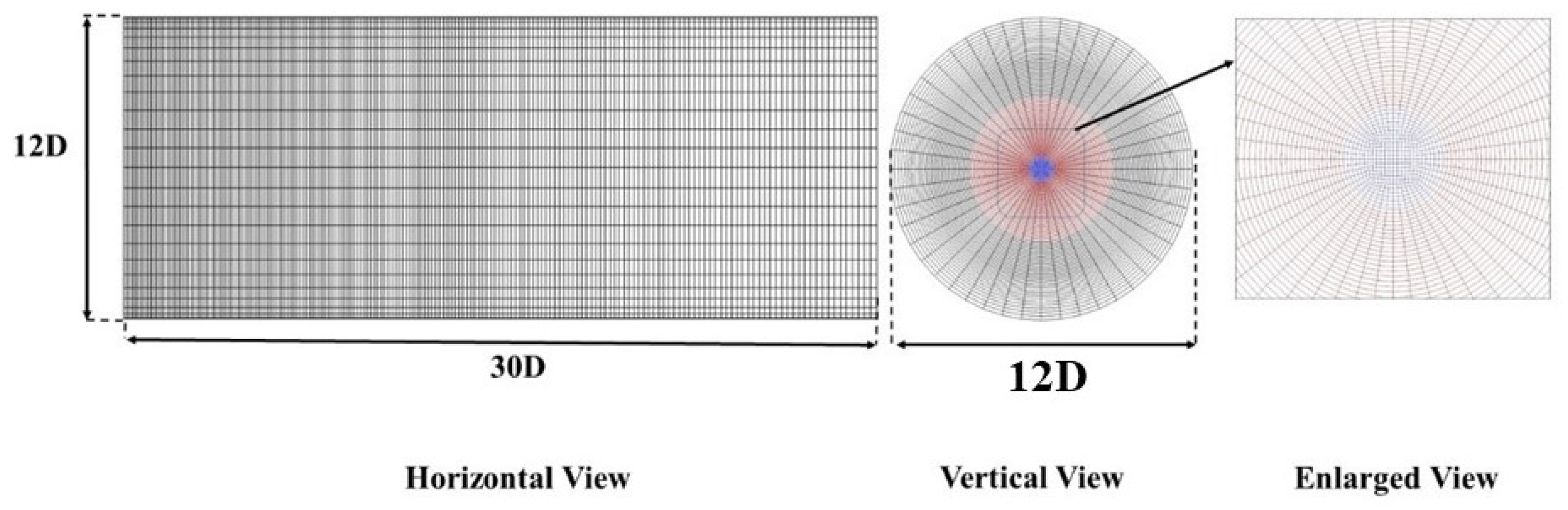
Figure 1. A sketch of the simulation domain and fine grid allocation. Blue area: main jet. Red area: pilot stream.
Energies 17 00252 g001
Figure 2. Instantaneous contour plots of the temperature and CO2 mass fraction distribution.
Energies 17 00252 g002
Figure 3. Centreline trends of the mixture fraction, temperature, axial velocity, and reactive species. Black solid line: mean value of the series model with a fine grid (i). Blue solid line: mean value of the series model with a coarse grid (ii). Square scatter: mean experimental data [34] (iii). Black dashed line: rms value of the series model with a fine grid (iv). Blue dashed line: rms value of the series model with a coarse grid (v). Triangle scatter: rms experimental data [34] (vi). Green solid line: mean value in reference [43] (vii). Green dashed line: rms value in reference [43] (viii).
Energies 17 00252 g003aEnergies 17 00252 g003b
Figure 4. Radial distributions of the mixture fraction, temperature, and reactive species. Black solid line: mean value of the series model with a fine grid (i). Blue solid line: mean value of the series model with a coarse grid (ii). Square scatter: mean experimental data [34] (iii). Black dashed line: rms value of the series model with a fine grid (iv). Blue dashed line: rms value of the series model with a coarse grid (v). Round scatter: rms experimental data [34] (vi). Green solid line: mean value in reference [43] (vii).
Energies 17 00252 g004
Figure 5. A sketch of the simulation domain and grid allocation. Blue area: main jet. Red area: pilot stream.
Energies 17 00252 g005
Figure 6. Radial trends of the temperature and species mass fractions. Black solid line: series model with a fine grid (i). Blue solid line: series model with a coarse grid (ii). Square scatter: experimental data [26] (iii). Green solid line: the Domingo et al. simulation [22] (iv).
Energies 17 00252 g006
Figure 7. Progress variable radial profiles. Black solid line: series model with a fine grid (i). Blue solid line: series model with a coarse grid (ii). Square scatter: experimental data [26] (iii).
Energies 17 00252 g007
Table 1. Sandia Flame D Simulation parameters and the comparison with previous studies.
ResearchTurbulent SGS ClosuresTurbulent Reacting LES ClosuresSimulation DomainGrid ResolutionChemistry Mechanism
Current studyDynamic eddy viscosity modelSeries model(15~30D) × 2π × 70DFine: 71 × 48 × 210 + 12 × 12 × 210 Coarse: 52 × 36 × 139 + 9 × 9 × 139 (Polar coordinates + o-grid)Jones–Lindstedt four-step mechanism
[43]Eddy viscosity modelEulerian stochastic field method40D × 40D × 84D68 × 68 × 106 (Cartesian coordinates)Jones–Lindstedt four-step
[44]SIGMA eddy viscosity modelDirect integration of chemical kinetics40D × 40D × 138D375 million tetrahedral elements (unstructured meshes)GRI 2.0 and 3.0
[45]Dynamic SmagorinskyMulti-environment PDF model(8~44D) × 2π × 80D101 × 64 × 197 (cylindrical coordinates)Reduced GRI 3.0
[46,47]Eddy–viscosity modelPresumed β-pdf and
Thickened flame approach
40D × 40D × 150D128 × 128 × 320 (Cartesian coordinates)GRI 3.0
[48,49]Dynamic SmagorinskyExtended flamelet/progress variable model26.5D × 2π × 80D160 × 64 × 256 (cylindrical coordinates)GRI 2.11
[36]SmagorinskyEulerian stochastic field method20D × 20D × 50D81 × 81 × 160 (Cartesian coordinates)Augmented GRI3.0
[50]Dynamic SmagorinskyLagrangian filtered-density approach20D × 2π × 80D256 × 128 × 32 (cylindrical coordinates)GRI-2.11
[51]Dynamic SmagorinskyConditional Moment Closure20D × 20D × 80D1.3M nodes (CMC grids)ARM2 chemistry
[52,53,54]Dynamic SmagorinksyHybrid Eulerian–Lagrangian MMC model35D × 2π × 35D512 × 55 × 32 (cylindrical coordinates)GRI-3.0
[55]One equation eddy viscosityEddy Dissipation Concept21D × 2π × 73D240 × 60 × 90 (cylindrical coordinates)GRI3.0 and Single-step mechanism
[56]SmagorinskyLagrangian Flamelet Model15D × 2π × 80D110 × 48 × 192 (cylindrical coordinates)GRI
2.11
[57]Modified kinetic energy viscosityFlamelet model15D × 15D × 80D101 × 101 × 91 (Cartesian coordinates)GRI
2.11
[58]SmagorinskyConditional Moment Closure8D × 8D × 80D96 × 96 × 320 (Cartesian coordinates)Meyer mechanism
Table 2. F3 Simulation parameters and the comparisons with previous studies.
ResearchTurbulent SGS ClosuresTurbulent Reacting LES ClosuresSimulation DomainGrid ResolutionChemistry Mechanism
CurrentDynamic eddy viscosity modelSeries model12H × 2π × 30HFine: 69 × 48 × 200 + 12 × 12 × 200 Coarse: 49 × 36 × 134 + 9 × 9 × 134
(Polar coordinates + o-grid)
Jones and Lindstedt’s four-step mechanism
[22,23]Vreman modelArtificially thickened flame8H × 8H × 16H194 × 194 × 306 (Cartesian coordinates)GRI 3.0
[61,62]SmagorinskyG-field4H × 4H × 20H64 × 64 × 296 (Cartesian coordinates)GRI-MECH 2.11
[63]Germano modelG-field and dynamic propagation model6H × 6H × 30H117 × 64 × 323 (cylindrical coordinates)GRI
[60]SmagorinskyEulerian stochastic fields5H × 5H × 15H56 × 36 × 112 (Cartesian coordinates)ARM for NO
[64,65]Dynamic SmagorinskyArtificially thickened flame4H × 2π × 20H94 × 64 × 300 (cylindrical coordinates)A two-step mechanism
[66,67,68]SmagorinskyDynamic modelling and Assumed PDF20H × 20H × 40H1.5 minion cells (Cartesian coordinates)Augmented reduction of GRI3.0
[69]Dynamic SmagorinskyDynamic thickened flame40H × 40H × 120HUnstructured meshesA single-step mechanism
[6]SmagorinskyDynamic thickened flame model40H × 40H × 120HUnstructured meshesA two-step mechanism
[70]Second momentTransported pdf4H × 4H × 12.5HLagrangian particle gridsLindstedt reduced mechanism
[71]Linear stress modelPdf method6.5H × 20H70 × 220 (2D simulation)Drm22
[72]SmagorinskyG-equation6H × 6H × 45H345,000 cells (cylindrical coordinates)Schmidt mechanism
Disclaimer/Publisher’s Note: The statements, opinions and data contained in all publications are solely those of the individual author(s) and contributor(s) and not of MDPI and/or the editor(s). MDPI and/or the editor(s) disclaim responsibility for any injury to people or property resulting from any ideas, methods, instructions or products referred to in the content.

