Abstract
The objective of this research paper is to apply a mathematical model to estimate and predict the economic growth of the Caspian countries in the period from 1995 to 2022. We use multiple regression by applying the OLS method to estimate the impact of global oil price, energy resource production per capita, trade, and renewable energy on GDP per capita. The mathematical approach uses fixed and random effects models to assess the overall impact of the independent variables on economic growth in this region and over the period analysed. This study also aims to investigate whether the explanatory variables are cointegrated in the long run; as such, we carry out several mathematical cointegration tests, namely the Pedroni and Johansen tests. The mathematical analysis is completed by the estimation of short- and long-run parameters using the stochastic VAR/VEC models, the impulse response function, and the causality test to assess economic growth in this region. This study’s main finding is that GDP per capita is increasingly influenced by its previous values, which is confirmed by considering lag 1 and lag 2. The results of the Granger causality tests identify several bidirectional relationships between GDP per capita and oil and gas production. These relationships are clearly positive evidence of the growth trend and progress of economic activity in the Caspian region. The practical implications of the study aim to promote and support the use of renewable energy sources. In this sense, policymakers in the Caspian countries should create favourable conditions for the transition to a green economy. An important aspect is the efforts of the government authorities to make their policies more environmentally friendly, as decarbonisation is a good practice in the current context of sustainability and related choices. As the Caspian countries are heavily dependent on conventional energy production, it is essential for them to increase their export earnings from energy resources via diversifying and strengthening new energy opportunities and partnerships.
1. Introduction
Currently, there is an increasing trend in the use of mathematical models to predict the consumption of energy resources over different periods and time intervals, across countries, industries, and sectors, using advanced econometric techniques—specifically, machine learning and deep learning tools [1,2,3,4,5,6,7].
The present research focuses on providing a multivariate analysis to examine the economic growth in the Caspian region and how this economic growth is influenced and affected by the turbulent movements of global energy prices, the dynamics and evolution of trade in energy products, and the potential domestic production of these energy resources (natural gas and oil). This study is also motivated by the increasing trend and inclination of energy-consuming countries (e.g., EU Member States) to diversify their import options and develop new energy partnerships. Thus, we believe that their endowment with these energy resources makes the Caspian countries relevant energy access points and relevant regional and global players. We also do not overlook the fact that the level of economic growth and development in these countries is closely linked to their potential to produce and export energy resources and to make significant efforts to discover and develop new oil and gas fields and reserves. Moreover, the importance of Caspian energy resources is extremely beneficial and necessary for the importing countries, especially in the current context of rapid and uncertain economic, social, and, above all, political changes and events.
Although there is a growing concern among researchers and academics to estimate and examine economic growth over different time intervals and across different countries or regions by applying multivariate analysis methods and techniques, we suggest that the current study is relevant in addressing the issue of the impact of energy resources on economic activity for the Caspian countries. More specifically, by developing a two-stage mathematical model, we were able to investigate how economic growth is increasingly sensitive and reacts differently depending on the variables used. At the same time, using multi-factor regression methods with cross-sectional data together with panel analysis techniques, it has been possible to highlight interdependencies on economic growth both for each Caspian country and at the level of this geographical region.
The structure of the paper is as follows: the second section presents the main findings according to the scientific literature; the following section presents the methodology and datasets used in the study. The fourth section presents the results. Section 5 presents the discussions and implications, and the last section presents the conclusions of the study.
2. Theoretical Background
In this section, we present the main theoretical and empirical contributions related to the estimation, modelling, and forecasting of natural gas and crude oil from the mathematical perspective of the models proposed and created. These energy resources continue to represent important points of interest in research activities, so we mention the valuable contribution of the study carried out by [8,9,10].
The central objective of these studies was to provide a rigorous and comprehensive analysis and synthesis of the scientific publications in the field. In this respect, these authors have chronologically presented different studies, classified according to the area of application, and used data, tools, and models to predict and investigate the causal relationship of natural gas consumption on economic activity in the countries analysed. We also believe that the paper provides a valuable background for future research in the field of energy and economic development, with a particular focus on the different forecasting tools and econometric techniques (i.e., mathematical models, statistical models, econometric models, dynamical systems models, and simulated annealing). In addition, the author draws attention to the need for theoretical development in this field and encourages future researchers to diversify and use new techniques, models, and data used to forecast natural gas supply, demand, production, and prices.
Thus, nowadays, more and more studies are investigating the causality relationships and possible effects of natural gas production and consumption on economic activity, economic growth, and economic development. In this regard, we mention the study conducted by [11], whose main objective was to assess the direct impact of natural gas consumption on economic growth in Tunisia over the period 1980 to 2010. The main aspects reported showed a long-term causal relationship between natural gas consumption, gross capital formation, and trade balance at the level of GDP, which should drive in the future the establishment, consolidation, and implementation of correlated energy and economic policies in economic activity. This consistently shows the tendency of net energy importing countries to use more and more natural gas as an alternative energy source to achieve environmental objectives (reduction of carbon dioxide (CO2) consumption), together with a high interest in studying its impact on economic activity [12,13,14].
Natural gas is an alternative energy source that has a positive impact on the environment (emitting less CO2 compared to other fossil fuels) and, in this sense, the study proposes a mathematical model (i.e., a Grey Model with an error latent information function) in order to forecast the annual production of natural gas consumption for the period 2016–2018 in the US and China. The novelty of this study is the extension of the classical Grey Model—GM (1,1)—via the inclusion of corrected outliers—GMCO (1,1)—such that the accuracy of the model improves remarkably. The evidence shows that this mathematical model was able to identify the series of variations and changes in natural gas consumption at the level of the two states mentioned. Specifically, in the short term, China will face a significant increase in its dependence on natural gas imports, with multiple implications for future global price trends. In the case of the United States, the increasing capacity for future natural gas exports to European and Asian countries has been demonstrated and confirmed by the current situation (e.g., the US exports an average of 5.6 billion cubic feet of natural gas per day).
The authors [15] have identified the bidirectional, long-run causal relationship between natural gas production, consumption, and economic growth in the seven Gulf Cooperation Council (GCC) countries. The causality analysis was conducted over the period 1980–2012 using multivariate mathematical models (i.e., FMOLS, DOLS models, Pedroni cointegration test, and Granger causality analysis) and the following independent variables: gross fixed capital formation, total trade in goods and services, labour force, and natural gas energy consumption. Furthermore, the study emphasises the important role of natural gas in reducing pollution and creating a clean and healthy environment in the region. The need to attract investments (natural gas energy projects and/or renewable energy investments) to generate long-term sustainable economic growth is another relevant aspect, according to the same study.
Using cluster mathematical analysis (i.e., analogue methods and fuzzy decision trees), ref. [16] drew attention to an innovative approach to long-term forecasting of natural gas consumption at the level of 79 countries in the period 1960–2019. Based on the macroeconomic variables used (GDP, GDP per capita, population, value added of industry to total GDP, CO2 emissions, energy intensity of GDP, share of natural gas consumption in the energy mix, HDD index, and annual natural gas consumption), it was found that the model leads to better results, in terms of increased performance and level of accuracy, in the analysis of forecasting annual natural gas consumption and production per capita. This proposed mathematical model can also be a valuable tool for forecasting natural gas consumption at the territorial level; the authors believe that its main advantage is the possibility of considering the cognitive uncertainty related to forecasts of socio-economic development, which are input variables to the model for forecasting demand for natural gas or other energy sources.
In addition, natural gas continues to be a primary energy alternative to support a clean and sustainable economic environment for Iran. This evidence was obtained by applying cointegration analysis (cointegration test, ARLD, FMOLS and DOLS models, and the Toda–Yamamoto Granger causality method) during 1991–2017.
Another study that examines both the causal relationships between economic growth and the use of energy sources, as well as economic growth and environmental pollution, is provided by [17]. Using panel data analysis for the period 1992–2013 for Georgia, Armenia, Azerbaijan, and Turkey, the results show the existence of a long-term causal relationship between the variables used (i.e., real gross domestic product (GDP), CO2 emissions, and energy use). Specifically, for Armenia, a unidirectional Granger relationship was found between energy use, CO2 emissions, and GDP, confirming the economic conservation hypothesis; for Georgia and Azerbaijan, a bidirectional relationship was found between energy use and GDP, confirming the feedback and growth hypotheses. In the case of Turkey, the validation of the neutrality hypothesis indicates that GDP and energy use are not cointegrated, implying that energy conservation policies would have no impact on real GDP. Furthermore, the policy implications of the study are aimed at maintaining and consolidating cooperative relations between Georgia, Armenia, Azerbaijan, and Turkey, which illustrates that energy has become an important precondition for the South Caucasus states to reduce poverty and promote regional economic growth and prosperity. Consequently, more and more countries are focusing on building a sustainable environment, and reducing CO2 emissions is one of their priorities. For these reasons, natural gas is becoming the best option for implementing a clean and low carbon energy system compared to traditional energy sources (especially fossil fuels). However, these priorities can only be met if government authorities establish a well-developed strategic energy plan, the core of which is a sound assessment and forecast of natural gas consumption, production, and price issues.
On the other hand, we identify valuable contributions on the significant impact of the global oil price on the general level of a country’s economic activity, as well as on the specific and individual level given by the market mechanism, the set of related industries, or the monetary-financial system. In this category, we include the study by [18], which assessed the response of the aggregate commodity market to oil price shocks and the impact of oil price shocks on China’s basic industries.
Thus, the authors were able to characterise the existing fluctuating movements and shocks of the global oil price and the resulting volatility by constructing composite mathematical indices composed of four major industries in China’s national economy: metals, petrochemicals, grains, and oil fats. Based on the ARJI, ARJI-ht, and EGARCH models, the results identify three types of volatility over the period 2001–2011, namely: expected, unexpected and negatively expected volatility. Moreover, the jumps in the price of crude oil are constant and have intensified in recent years, which can be explained by the increasingly sensitive response of Chinese industries, while the investment risk in these industries is becoming higher. Thus, a policy implication of this study focuses on starting to use technological mechanisms to produce renewable energy, which in the future will lead to a decrease in the import of traditional energy resources and additional protection against the volatility of the prices of these energy products at the level of China.
The authors of [19] concluded that GDP, as a macroeconomic indicator, is the most important factor contributing to (and directly affecting) increases in oil consumption. They captured this aspect by conducting a mathematical analysis among the world’s most important and complex economies—Japan, the US, India, and China—over the period from 1970 to 2008. In other words, it has been shown that oil demand is inelastic to price and perfectly elastic to income levels throughout the panel; surprisingly, however, there is a pseudo-demand in Japan. This can be explained by a number of factors; namely, an increase in population alone does not ensure demand for more oil. It must be supported by an increase in the purchasing power of the country’s citizens or the impact of technological progress aimed at major changes in the field of energy resilience (from fossil fuels to alternative energy sources such as nuclear energy).
The main objective of policymakers is to adopt interrelated and interconnected energy policies and strategies to improve the progressive process of economic development. On the other hand, the inverted U-shaped relationship between oil consumption per capita and GDP per capita was statistically found for 61 countries grouped into OECD, non-OECD, developing, and other developed countries [20]. The analysis was carried out over the period 1990–2008 using the common effects model, the fixed effects model, and the random effects model. The same study also concluded that oil consumption is prone to significant growth over a long period of time, explained by rapid population growth in most developing countries, calling for the development of policies based on the use of renewable resources, green technologies, and major investments to make oil production more efficient and increase its output.
A more recent study was conducted by [21], whose main objective was to test and examine the causal relationships between oil, natural gas, and economic growth. Specifically, they have used the following explanatory variables in terms of reserves, production, exports, and prices for each of the energy resources mentioned. The methodology used by the authors is based on specific mathematical models for the five Caspian countries in the period 1997–2015. The main implications of the study showed that oil and natural gas have a strong influence on economic activity in this region, that there is a unidirectional Granger relationship between GDP and oil prices, and the fact that any changes in natural gas prices and natural gas exports affect economic growth in this region.
It is also noted that the Caspian countries will be able to intensify and progressively consolidate their energy trade relations (especially within European countries) by developing mutually beneficial military, economic, and social cooperation objectives. On the other hand, there are specific studies aimed at identifying the main factors influencing the production and consumption of natural gas and oil, assessing export routes, and progress in improving the energy systems within the Caspian countries (Azerbaijan, Iran, Kazakhstan, Russia, and Turkmenistan).
First, studies estimating the production potential of the two energy resources [22,23,24,25] deserve our attention. The findings suggest that oil and gas production in this region is explained by and depends on the degree of FDI attraction, global oil price, export route capacity, political conflict, and proven oil and gas reserves. Attention is also drawn to the diversification of export options for Caspian resources, as well as the consolidation of new ways of developing European markets in the immediate future.
Secondly, we identify studies that assess the impact of oil and gas pipeline planning in Caspian countries [26,27,28]. These studies include the application of decision-making methods and several mathematical models to assess and identify the best export routes for Caspian energy resources (i.e., a hybrid group decision support system, the Delhi method, SWOT analysis, a preference-ranking organisation method for enrichment evaluation, and the Geometrical Analysis for Interactive Assistance plane).
Thirdly, there are studies that promote the use of renewable resources—solar energy, wind energy, hydropower, biomass, or other renewable energy sources to achieve a clean and CO2-emission-free energy system in the Caspian region [29,30].
The studies [31,32,33] suggest that energy system efficiency is mainly based on increasing and maximising the share of renewable resources in the total energy sources. The results showed a significant increase of about 40% of renewable energy sources in electricity generation within the Iranian provinces. At the same time, the scenario analysis concluded that the energy system in this Caspian country will become more efficient by improving the efficiency of power plants by 2% per year and increasing the capacity of hydropower by 10% per year in the period 2020–2030.
The author of [34] conducts a relevant study that uses multivariate regression methods to investigate the causal relationship between economic development and the environment. The aim of the paper was to investigate the role of the economy, finance, and institutions in environmental degradation. Therefore, from a methodological point of view, a panel sample of a number of EU and MENA countries was created, and a panel data analysis was conducted over the period 1990–2011. However, the empirical results suggest that the EKC (i.e., the Environmental Kuznets Curve hypothesis) of the EU and MENA shows a monotonic growth relationship between pollution and per capita income instead of an inverted U-shaped curve. From this perspective, the author draws attention to the fact that the emergence of such an inverted U-shaped curve is not a spontaneous result of economic growth, but rather depends on the existence of stringent environmental institutions and policies.
A relevant aspect found in the literature is the analysis of the relationship between the use of renewable energy sources, economic growth, and economic development. Studies by [35,36] go in this direction. The authors of these papers make a convincing case for the impact of renewable energy on economic progress and welfare by conducting a bibliometric analysis of publications on the subject between 2008 and 2021. The results show that there is a lack of studies in the literature analysing the causal relationship between renewable energy and economic development, as well as less focus on developed countries. It also showed a preference for the use of quantitative research methods in the study of this issue in economics.
Using stochastic panel-level models for more than 130 countries over the period 2008–2014, ref. [37] examined the impact of renewable energy consumption on the level of economic growth and productivity. The main findings suggest that a sequential and systematic increase in the use of renewable energy resources has a positive impact on productivity and thus generates economic growth. At the same time, while this is manifested in different ways depending on the level of development of each country analysed, attention was drawn to the beneficial effects of promoting and supporting renewable energy on environmental and energy security issues.
Similarly, we find a recent study performed by [38]. The aim of this study was to determine the causal relationships between the level of carbon dioxide emissions, renewable energy sources, and economic growth (expressed as GDP per capita) for Romania in the period 2000–2021. Following the application of the ARDL model and robustness tests, it was concluded that there is a negative causality relationship between CO2 emissions and GDP, while renewable energy resources have a positive impact on the level of economic growth in both the short and long term, indicating significant changes in the diversification of energy sources and the reduction of fossil fuel dependency for Romania in the immediate future.
Other authors [39] conducted a multivariate analysis of the significant role of renewable energy sources in economic growth for two European countries, Sweden and Poland, during the COVID-19 pandemic. The evidence showed that economic growth and development, as well as the share of renewable energy sources in gross marginal energy consumption, are the variables between which mutual interaction occurs in these two countries. The results also confirmed that the developed world’s economic growth prospects over the longer term, as measured by GDP, are dependent on renewable energy use.
Another interesting aspect found in the literature is the concept of inclusive growth. In this sense, this objective can be achieved by promoting and increasing the use of renewable energy sources, where this energy transition requires support and backing from government authorities and policy makers. The research carried out by [40] provides a focus on the study of inclusive economic growth that can be explained by renewable energy sources, energy trade, and indicators measuring the effectiveness of political governance for the 26 EU Member States over the period 2011–2020. As a result, the empirical evidence suggests that there is a non-linear, statistically significant relationship between e-governance and affordable and clean energy.
3. Research Methodology
The main objective of our study is to develop a mathematical growth assessment model that can be applied at the individual level, i.e., for each of the Caspian states under consideration, and at the aggregate/holistic level for this geographical region (i.e., the Caspian region). From this perspective, mathematical analysis is carried out over the period 1995–2022, based on the use of time series for each variable included in the model, for Azerbaijan, Iran, Kazakhstan, Russia, Turkmenistan, and Uzbekistan. The measurement and estimation of economic growth is explained by the level of GDP per capita, which is used as the target or dependent variable.
Our model also takes into account the following independent/explanatory variables over the period analysed: the global benchmark price of oil (i.e., Brent crude oil spot prices), domestic gas and oil production per capita, trade dynamics (given by the sum of total exports and total imports), and the trend in the share of renewable energy resources. The mathematical form is presented in Equation (1).In addition, the variables included in the mathematical model used have been selected on the basis of information available in the literature [41,42,43] and are strictly related to the increasing impact and influence of energy prices on the economic growth rate.
At the same time, following global initiatives on sustainability and the environment, recent studies [44,45,46] have shown that net-energy-producing and net-energy-exporting countries are becoming increasingly aware of environmental issues and, as a result, are showing a greater/greater willingness to reduce the consumption of greenhouse gas emissions and increase the share of renewable resources in their total domestic energy production. For each variable, data has been taken from the World Bank database, Our World in Energy, and the Statista database.
where: represents the country and represents the time (.
Table 1 provides a detailed overview of all variables used. Table 2 provides the statistical descriptions of the variables included in the panel and Appendix A provides the statistical descriptions of the time series for each Caspian country.

Table 1.
Variable presentation, definition and data sources.
Table 2.
Descriptive statistics of variables at the sample level.
As a first aspect, we note that the total number of observations is 168 and that the variables included in the model are extremely different in terms of mean, median, and standard deviation from the mean. More specifically, we observe that GDP per capita deviates the most from the mean, followed by domestic oil and gas production per capita, while renewable energy and trade dynamics deviate the least from the mean.
Looking at the statistical indicators describing the distribution of each variable, it can be seen that GDP per capita, natural gas production, and the series describing the evolution of trade have a leptokurtic distribution over the period analysed, which is confirmed by the values of the kurtosis coefficient greater than 3/00, while the rest of the variables have a platykurtic distribution, with the values of the kurtosis coefficient in both cases being less than 3.00 (the specific value of a normal/symmetric distribution).
With regard to the Skewness indicator, which describes the degree of asymmetry for each distribution, it can be seen that GDP per capita, the world oil price, and natural gas production per capita have a positive skewness, all having a long right tail and higher values of these variables, while only oil production per capita has negative values of the Skewness coefficient, indicating the existence of a long left tail and lower values. In addition, looking at the absolute values of the Jarque–Bera normality test, the degree of heterogeneity of the variables included in the model is highlighted, as they tend to deviate from a normal distribution N (0,1), which is confirmed by p-values that are less than 5%, so the null hypothesis (the series has a normal distribution) can be rejected.
All variables included in our model were transformed and presented in logarithmic form to obtain robust and appropriate mathematical results. The mathematical analysis was further divided into two phases. In the first phase, we applied the model set up to examine growth in each of the Caspian countries over the period 1995–2022 and we constructed six mathematical models that describe the impact of the explanatory variables on the GDP per capita in each of the Caspian countries analysed. In this respect, we first tested the mathematical assumption of stationarity using the ADF and PP unit root tests, the general form of which is shown in Equation (2).
where ; is the individual constant term, is the slop parameter; represents the stationary distribution, and and are I(1) variables.
Then, it was possible to apply the proposed mathematical model by applying multivariate regression for each individual Caspian country. The estimation of regression coefficients was performed using the least squares method, and the general form for each model is presented in Equation (3).
where is analysed individually and successively for Azerbaijan (Model 1), Iran (Model 2), Kazakhstan, (Model 3), Russia (Model 4), Turkmenistan (Model 5), and Uzbekistan (Model 6) from 1995 to 2022; represents the observations for each mathematical model; is the intercept; represent the estimated coefficients for the independent variables; and is the error term.
Within each multiple regression, we used control variables given by the first lag/decay of the explanatory variables (lag 1 variables) to investigate the dependence and prediction of GDP per capita in its dynamics for the analysed countries [47,48,49].
In our study, the proposed mathematical model for estimating and forecasting the economic growth rate among the Caspian countries has been achieved by applying the multiple regression method, or multifactor regression. The popularity of this econometric method is extremely well established, as it is often used and applied in various and diverse scientific fields and problems of interest.
At the same time, multivariate regression is the most used technique in the social sciences to measure the impact of independent (or explanatory) variables on a dependent variable. In general, regression—specifically, ordinary least squares (OLS) regression—assumes that the dependent variable is continuous [50,51].
It can be used to estimate the coefficient of each independent variable and test the extent to which it explains the variation in the dependent variable. In addition, multiple regression allows us to form hypotheses about the effects of different variables and to compare the fit of different models.
The ability to capture the complex and multifaceted nature of real-world phenomena is one of the main advantages of multiple regression. Including multiple independent variables allows one to account for more factors that influence the dependent variable, reducing error and bias in estimations. For example, multiple regression also allows us to control for confounding variables, which are variables that affect both the dependent and independent variables and can distort the true relationship between them.
From a methodological point of view, we investigated multivariate analysis in the following aspects: ensuring correct specification of the regression model, zero variance of independent variables, zero mean of the error, normal distribution of the error term, uncorrelated independent variables with the error term, and constant variance of the error term.
Therefore, we first tested the estimated coefficients for each economic growth model using the statistical t-test. According to [50,51], this test is a ratio that quantifies how significant the difference is between the means of two groups, considering their variance, or distribution, and the specific hypotheses: and .
Further, the F-test and the value of the adjusted coefficient of determination were also used to check the reliability of the economic growth model. In regression analysis, the F-test is a test of the hypothesis that all model parameters are equal to zero. It is used in statistical analysis to compare statistical models fitted to the same underlying factors and data set to determine which model is the best fit. The F-test is a measure of the ratio of the variances and was developed by Ronald A. Fisher (hence, the F-test).
According to [52,53,54], the adjusted form of R-squared (adj. R2) has been considered in predictive modelling as one of the most widely used and reliable statistical tools to test the goodness of fit of a model or to compare the performance of different models. In fact, the adjusted form of R-squared (adj. R2) is adj. (adjusted) R2 is considered a basic and essential tool for making a final decision about the relationship between the dependent variable and a set of explanatory variables.
In addition, the White test [55], the Breusch–Pagan–Godfrey test [56], and the Jarque–Bera test [57] were used to test the assumptions of the homoscedasticity of errors and normal distribution of errors for the proposed models of our analysis. The White and Breusch–Pagan–Godfrey tests are the main statistical tests used to determine whether the variance of the errors in a regression model is constant; that is, for homoscedasticity under the following hypotheses: and , and if the p-value is greater than the 5% level of statistical significance, the errors are homoscedastic. The Jarque–Bera test is a reference test for the normality of errors based on the following assumptions: the errors are normally distributed; and the errors are not normally distributed.
The second stage of the model was to examine the degree of interdependence for GDP per capita between the explanatory variables at the level of the Caspian region over the period 1995–2022.
However, it was necessary to test and examine the interrelationships between GDP per capita, global oil prices, trade, use of renewable energy sources in the energy mix, and total domestic oil and gas production (on a per capita basis) for the entire Caspian region. Our approach is holistic and comprehensive in measuring and predicting economic growth in this strategic region. Thus, we have chosen to use two econometric methods specific to panel analysis: the fixed effects regression model and the random effects regression model.
We emphasise that these econometric models are among the most popular and widely used research methods in economics and finance because of their ability to capture the interdependencies and autocorrelation of time series. Regression panel data is a combination of cross-sectional and time series data where the same unit cross-section is measured at different points in time.
In fact, panel regressions provide better estimation and prediction because they have a double index for their variables: the —index, which shows the cross-sectional dimension, and the —index, which shows the temporal dimension. For this reason, using the panel methodology approach, we can estimate the impact of a single coefficient on the independent variables specified over time and by entity, and determine and estimate these regressors [58]. An additional advantage comes from the fact that the panel methodology can estimate the coefficients in a dynamic and modified way, where they can be controlled by individual fixed effects.
The fixed effects model tests for the presence of individual effects, and the component may be correlated with the regressors , but the assumption remains that there is no correlation between and the random component of the error . Therefore, the fixed effects regression model also assumes that the errors are independent and identically distributed after removing the fixed effects, and takes the following form:
where is the error component that is specific to each cross-sectional dimension and reflects the differences between the countries; is the dependent variable (in this case, the natural logarithm of GDP per capita); represents the cross-sectional dimension (in this case, the Caspian countries); represents the temporal dimension (; is the intercept that does not change over time; represents the estimated coefficients; is a vector including the independent and explicative variables; and is the error terms.
The second panel data regression model is the random effects model. This model predicts how variables may be related over time and between individuals. In the random effects model, the difference between the intercept terms is compensated by the error terms of everyone (in our case, for each country). The form of this model is as follows:
where means the error term for each country.
On the other hand, the results of the multivariate analysis of economic growth in the Caspian countries carried out in this study need to be further investigated and evaluated. From this perspective, the reliability of our models’ results is ensured by conducting both accuracy and diagnostic tests.
From a mathematical point of view, we chose in this case to apply panel analysis by creating a balanced panel that included data for each state (cross-sectional dimension) and data for each year (temporal dimension). First, we applied unit root tests with panel/panel-type data in order to test the hypothesis of stationarity of the variables and to see their degree of order: I (0) or I (1). It was also necessary to see whether the variables used are cointegrated, i.e., whether they are correlated in the long run over the period analysed. For this reason, the cointegration hypothesis was tested using the Johansen and Pedroni tests, and the mathematical formula is shown in Equation (6).
where is the first difference, is the series in our panel in the time , is the number of lags, and is the distributed random variables.
If it was confirmed that the variables are cointegrated, we applied the vector error correction model, a model that allowed us to examine the deviation of the short-run and long-run coefficients from equilibrium. Alternatively, we also used the mathematical cointegrated regression models FMOLS and DOLS to investigate in the long-run relationships between variables and to estimate the regression coefficients of a panel regression model. The literature [59,60,61,62] suggests that the FMOLS model is superior to other regression models because it overcomes the problem of serial correlation and endogeneity of variables.
Otherwise, if the variables are not cointegrated, we used the VAR model and two other panel regression models, the fixed effects model and random effects model, to see how GDP per capita is affected by the explanatory variables in the short run. In Equation (7), the specific form of these mathematical regression models is illustrated.
where represents the country (); indicates the time (); is the constant term; are the coefficients for each independent/explanatory variable; represents the country-specific error component, which varies between countries; and indicates the error term, which captures the impact of unobserved variables that vary both across countries and over a period of time.
Equation (8) shows the general form for the VAR model, and the following Equations (9)–(14) show the specific form of the VAR model for the variables under analysis.
where is a -variate random process; is time period; is a positive integer; are fixed coefficient matrices; is a fixed vector of intercept terms; and ,…, is -dimensional white noise or error terms.
It should be noted that for these equations, the dependent variable is a function of its lagged values and the lagged values of the variables included in the model. Here, are the intercept terms for each equation; is the lag length for the VAR model; are the estimated short-run coefficients for each equation in the VAR model; and is the error term for each equation.
Regardless of whether the time series are cointegrated or not, testing the robustness and diagnosis of these regression models using panel data is an essential step in the mathematical approach.
The final step is to identify the mathematical Granger causality, which predicts a time series based only on its own past values, and that of the full model, which also includes the past values of another time series, and to perform the analysis of the impulse response functions resulting from the VAR model design.
In our case, it is important to see whether the economic growth rate can be driven by the dynamics of the world oil price, the share of renewable energy sources, the domestic production of oil and natural gas, and the evolution of trade in the immediate future.
The whole mathematical process was carried out in EViews 12, and the methodological steps are described in Figure 1.
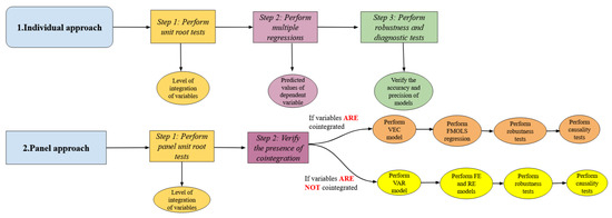
Figure 1.
Two-stages mathematical model design. (Source: Authors’ work).
4. Results
4.1. Results after the Application of the Mathematical Model at the Individual Level (for Each Caspian Country)
In this section of the paper, we comparatively present the results obtained from the implementation of the proposed mathematical model, focusing on the interdependence relationship between GDP per capita and global oil prices, domestic oil production, domestic gas production, share of renewable energy sources, and trade dynamics for each of the Caspian countries analysed (i.e., Azerbaijan, Iran, Kazakhstan, Russia, Turkmenistan, and Uzbekistan) over the period 1995–2022. Thus, we first focus on the mathematical testing of the stationarity assumption of the time series used for each country. In this respect, mathematical tests have been applied to determine the degree and order of integration of the time series to satisfy the condition of stationarity.
Table 3 shows the unit root tests commonly used in the statistical and mathematical analysis of time series proposed by [63,64,65,66]. In our case, it was possible to show that the time series analysed are not stationary in level, since they satisfy the condition of stationarity after the first difference.
Table 3.
Unit root tests results for each country.
Thus, for each of the six countries, the time series are integrated of type I (1), an aspect confirmed by probability values converging to 0.000, and the tests are statistically significant at the 5% level of significance. Moreover, the fulfilment of the stationarity condition of the time series for each analysed country is an important aspect in obtaining robust and appropriate results from our model.
Going further, we can successfully apply the proposed mathematical model to each country, and we can capture a number of empirical insights from the mathematical analysis in a comparative perspective. The results of the estimated coefficients from the application of multivariate linear regression for the six mathematical models are presented in Table 4, while Table 5 shows the main robustness/accuracy indicators and diagnostic tests for these applied mathematical models.
Table 4.
Results of estimated coefficients from individual multiple regression (GDP_CAP as dependent variable).
Table 5.
Results of robustness and diagnostic tests from individual multiple regression (GDP_CAP as dependent variable).
Specifically, for Azerbaijan (Model 1), GDP per capita is statistically significantly (at the 5% level) influenced by trade dynamics, domestic oil production per capita, and the share of renewable energy sources, as well as domestic natural gas production with one lag. Thus, the coefficients of these variables are statistically significant at least at the 5% confidence level, and the impact of these variables on GDP per capita is in the same direction and positive. Specifically, a 10% increase in domestic oil or gas production increases GDP per capita by around 8% and 3.60% respectively.
The mathematical model is also valid and correct, as shown by the very high value of the adjusted coefficient of determination, around 0.98, and the high and statistically significant value of the F-test, which confirms that GDP per capita is explained and influenced to a high degree by the variables included in the model. At the same time, the diagnostic tests indicate that the model is homoscedastic, does not suffer from autocorrelation or serial correlation, and that the errors are identically and normally distributed, aspects confirmed by the Jarque–Bera test, the LM test, and the Breusch–Pagan–Godfrey test.
Similar results are obtained for Iran (Model 2). The mathematical model is correctly specified, it does not suffer from heteroskedasticity and autocorrelation, and GDP per capita is explained by more than 95% of the variation in the independent variables.
However, in contrast to Azerbaijan, it was observed that the world oil price affects the level of GDP per capita; if it increases by 10%, GDP per capita increases by only 0.64% in the short run. At the same time, for Iran, it was found that a 10% increase in domestic oil and gas production changes the level of GDP per capita in the same direction, increasing it by 3.40% on average. These results suggest that the short-term evolution of trade in Iran leads to a decrease in GDP per capita of around 1%, which can be explained by significant differences between exports and imports and the existence of a negative short-term trade balance/short-term trade deficit. However, if the model also considers the first-order trade lag, the situation changes and GDP per capita is positively affected, increasing by about 0.90%.
The results obtained by applying the model for Kazakhstan (Model 3) indicate that the use of renewable energy sources is a driver for the growth rate of GDP per capita, with an upward trend of up to 2%. Like the results obtained for Iran, it was also observed that a 10% increase in the world oil price leads to a 1.48% increase in GDP per capita. The proposed mathematical model for Kazakhstan is adequate and robust, being correctly constructed and stable in terms of the absence of heteroskedasticity and the normal distribution of errors.
Analysing the situation for Russia (Model 4) and Turkmenistan (Model 5), the mathematical model is adequate for estimating and measuring economic growth, with the independent variables explaining more than 95% of the level of GDP per capita. For Russia, the specific results show that GDP per capita is directly and positively influenced by domestic oil consumption, which is captured by the estimated statistically significant coefficient at the 10% level.
The situation is no different for Turkmenistan, where the mathematical model shows a decrease in GDP per capita of about 18%, influenced by a 1% increase in the share of renewable energy use. This can be explained by the lack of development of the regulatory framework for energy conservation and efficiency, as well as for solid waste management as a renewable energy resource. In addition, the model is homoscedastic and stable for both Caspian countries analysed according to the Breusch–Pagan–Godfrey test.
Finally, the mathematical model has also been applied to Uzbekistan (Model 6). The results obtained and presented in Table 4 and Table 5 indicate that GDP per capita is indirectly influenced by domestic oil production per capita, trade dynamics, and the share of renewable energy use, with the estimated coefficients being statistically significant at the 5% and 10% significance levels. It was also found that a 10% increase in domestic natural gas production per capita (in the form of lag 1) tends to increase GDP per capita by about 2.90%, which is confirmed by the fact that Uzbekistan is one of the world’s largest natural gas producers, producing about 60 billion cubic metres (bcm) annually, of which 35–40 bcm are supplied by Uzbekneftegaz JSC [26,67,68].
It is interesting to note that the world oil price, in the form of lag 1, leads to a decrease of this indicator by 0.80%, which is explained by the unstable financial situation of the country and the insufficient introduction of resource- and energy-saving technologies, factors which have increased technological losses and increased the frequency of interruptions in the supply of fuel and energy resources. These results are complemented by the positive impact of trade on GDP per capita, which is very positive given the extensive reforms undertaken in recent years to strengthen the energy industry and the extension of energy cooperation to EU Member States.
As in the case of the other countries analysed, the mathematical model applied for Uzbekistan is stable and has no serial correlation, the errors are normally distributed, and the variance of the error term in each regression model is constant. Consequently, the proposed mathematical model was found to be suitable, adequate, and robust to assess the interdependent relationships between GDP per capita and the explanatory variables for each Caspian country during the period from 1995 to 2022.
Therefore, by estimating and forecasting GDP per capita values in the six Caspian countries, we draw attention to the fact that domestic production of natural gas, oil, and renewable resources are the main drivers that boost overall economic performance [69].
Essentially, it can be confirmed that the Caspian countries are significant regional and global producers and exporters of energy resources, and that they are undergoing a series of reforms and domestic policies to continuously improve their energy system.
4.2. Results of the Mathematical Model Applied to the Caspian Sea Region (the Panel Mathematical Approach)
In this section, we present and discuss the results obtained from the application of the proposed mathematical model from a multivariate and panel perspective. For this purpose, the model examines the impact of the world oil price, domestic production of energy resources, and trade developments on the level of GDP per capita in the Caspian region.
Thus, the panel consists of the six Caspian countries (i.e., Azerbaijan, Iran, Kazakhstan, Russia, Turkmenistan, and Uzbekistan) and the data for each variable examined are available for the period 1995–2022. From this point of view, we can confirm that the panel is balanced, equilibrated, and fixed and that the study of data in a panel structure affords the joint analysis of cross-sectional observations (regions, countries, sectors, households, firms, etc.) over several time periods. At the same time, an initial argument in favour of using the proposed mathematical model with panel data comes from the fact that it can capture individual peculiarities, invariant structures within a unit or at a given point in time, thus reducing or eliminating the distortions induced by the aggregation of data.
The literature [70,71,72,73,74] provides strong arguments for the use of mathematical analysis with panel data, and among the main issues raised are the provision of more information by capturing individual variability, reducing multicollinearity of variables, and increasing the number of degrees of freedom—and thus the power of the tests, and hence the confidence in the results—as well as increasing the efficiency and consistency of the resulting estimates and providing better analysis of the dynamics of structural adjustments.
To this end, we used the methodology specific to autoregressive models in the multivariate VAR/VEC form and go through several steps, including stationarity tests of variables, cointegration verification, VAR/VEC coefficient estimation, impulse response functions (IRFs) and Granger causality tests.
The results of the stationarity tests are presented in Table 6. This test was applied to each variable included in the model, indicating whether the time series used had a unit root. It was observed that the variables are not stationary at level I (0), but they became stationary after the application of the first difference, the tests applied being statistically significant at the 1% level of significance.
Table 6.
Panel unit root tests results.
This indicates that they are of I (1) form and that our model can be analysed by successfully applying the VAR/VEC methodology.
Given that the variables are I (1), a necessary condition in our analysis is to test the hypothesis of cointegration between the variables, or rather to test a long-run association between them. In this regard, the cointegration hypothesis was tested by applying the Pedroni test, where 9 out of 11 tests (i.e., panel V-statistic, panel rho-statistic, panel pp-statistic, panel ADF-statistic, group rho-statistic, group PP-statistic, and group ADF-statistic) confirmed that the variables are not cointegrated and, therefore, that there is no long-run relationship between the variables.
Thus, the null hypothesis of no cointegration is confirmed, as indicated by the probabilities of the statistical tests that are greater than the 5% confidence level, and in our case the VAR model is recommended in the proposed mathematical analysis. The results of the Pedroni cointegration test are presented in Table 7.
Table 7.
Results of cointegration panel test.
Furthermore, the VAR model was implemented with 2 lags, which was validated by the four statistical indicators (i.e., Akaike information criterion, Hannan–Quinn information criterion, final prediction error, and LR test) for determining the optimal number of lags.
The results of these statistical indicators on the VAR lag order selection criteria are presented in Table 8. Similarly, the cointegration hypothesis could also be tested using the Johansen cointegration test, the results of which are presented in Table 7 above. Once again, it is confirmed that the variables do not show a long-run relationship, since the values of the two cointegration tests (i.e., trace and maximum eigenvalue) are both lower than the critical values at the 5% significance threshold, thus calling for the application of the VAR model in our panel.
Table 8.
The results of the VAR lag order selection criteria.
Table 9 and Table 10 show the results of estimating the short-run coefficients using the VAR model. First of all, it should be noted that in the short run, GDP per capita is influenced by its previous values, i.e., a 1% change in GDP per capita is associated with a 1.52% increase in the previous value of GDP per capita at lag 1. However, this changes when we consider a two-period lag of GDP per capita, which shows a decrease of around 0.52% in the short run.
Table 9.
Short-run coefficients panel VAR results.
Table 10.
Robustness and diagnostic tests panel VAR results.
These results are supported by empirical evidence found in studies by other authors/researchers [21,22,23,75,76,77,78] that show that GDP per capita is increasingly influenced by its previous values and reacts differently depending on its evolution and tendency to increase or decrease. Again, it was observed that gas production per capita has an impact on GDP per capita over the analysed period; a 1% change in GDP per capita is associated with a 0.06% decrease in gas production per capita with lag (1).
As an alternative to the results captured by the VAR model, we applied panel data regression models in the form of a fixed effects model and a random effects model to investigate the short-run impact of GDP per capita over the period under study across the Caspian region.
The main findings of the fixed effects model (FE model) indicate that the level of GDP per capita is statistically significantly influenced by the dynamics of trade, the world oil price, oil production, and natural gas production expressed per capita.
In this geographical area, a 10% change in trade was found to reduce GDP per capita by about 3.6% in the short term, which can be explained by the different evolution of the trade balance specific to the countries that make up this area.
In addition, the use of renewable energy sources was found not to affect the dynamics of GDP per capita in the short term, as confirmed by the estimated statistically insignificant coefficient at the 5% significance threshold, which draws attention to the lack of measures and energy policies to promote the transition to a green economy and a clean environment. At the same time, the positive impact of the world oil price is felt in this region, as it leads to an increasing trend in GDP per capita of about 4.10%.
Regarding the robustness of the applied regression model, it was found that it is adequate and appropriate to estimate GDP per capita at the Caspian region due to the high value of the statistical F-test and the extremely low probability associated with it (p-value is less than 1%).
Applying the random effects regression model, it was found that 67% of GDP per capita is explained by the explanatory variables, which are also directly influenced by oil and gas production and indirectly (negatively) by the evolution of trade over the period analysed.
We have also proposed to investigate which of the two panel regression models (FE and RE models) is more appropriate to measure GDP per capita over the period 1995–2022. Several diagnostic tests were used for each panel and the results of these panel regression models and specific tests are presented in Table 11.
Table 11.
Panel regression models results (GDP_CAP as dependent variable).
The Hausman test was used to decide between the fixed effects panel and the random effects panel. The Hausman test indicates the following hypotheses: for H0, there is no correlation between the estimators, and for H1, there are random effects.
Thus, the results of the Hausmann test suggest that the fixed effects regression model, with a p-value of less than 5%, is more appropriate for investigating the impact of the explanatory variables on GDP per capita.
The results of the analysis carried out are complemented by Granger causality tests. To implement the panel causality test, we chose the Dumitrescu–Hurlin test [58], which assumes that the regression coefficients in the bivariate regressions resulting from the Granger causality tests can vary across cross-sections.
We performed this causality test using the optimal number of lags (in our case, two lags) and we wanted to focus on how the variables interact with each other and how they affect the level of GDP per capita in the future.
The results of the Dumitrescu–Hurlin test are presented in Table 12 and confirm that there are bidirectional causal relationships as follows: trade and GDP per capita, oil production per capita and GDP per capita, and world oil price and oil production per capita.
Table 12.
Results of panel causality test.
These bidirectional relationships reinforce the idea that the Caspian countries are increasingly seen as globally relevant and important in the production and trade of their energy resources.
In addition, they are responding to changes and shifts in energy reference prices by being able to reorganise and manage their current and future supply and expected demand, but also by finding possible levers and instruments strictly related to global price fluctuations and swings (i.e., price volatility risk management).
Other causal relationships were found between GDP per capita and world oil prices (unidirectional); GDP per capita and trade (unidirectional); and GDP per capita and natural gas production per capita (unidirectional).
Interestingly, the world oil price causes a Granger-linked trade dynamic; this unidirectional relationship points to the following: when the benchmark price is higher, exports also tend to increase, thus affecting economic activity.
The final step in our analysis is to uncover the impulse response functions (IRFs) for GDP per capita in the Caspian region. These functions show the impact of a shock originating in an independent variable on the dependent variable, on an individual basis.
The results (Figure 2) show that a single shock to GDP per capita from the world oil price decreases progressively from the first period to the end of the forecast period and remains stable between the two-and four-year periods. It also shows that shocks to GDP per capita will have a negative impact on trade, which falls sharply into negative territory in at least two years. In addition, shocks to GDP per capita will have asymmetric impacts on gas production per capita and oil production per capita and the values are expected to remain stable over the entire 10-year forecast period. Nonetheless, a single shock to GDP per capita initially increases the use of renewable energy.
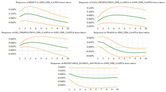
Figure 2.
Response to Cholesky One S.D. Innovations ± 2 analytic asymptotic S.E.s. Note: The line in green represents the response of the independent variables to the GDP per capita as our dependent variables. The lines in orange represent the asymptotic standard errors at the 5% level of confidence. (Source: Authors’ own calculations).
This positive response declines sharply until the second period, when it reaches its steady state value, from where it remains negative from the third to the tenth period. The results of the impulse-response analysis are ultimately consistent and reasonable. Recent events have become increasingly imprecise and unpredictable. They have had a negative impact on the level of GDP per capita, trade dynamics, and domestic production of energy resources in the countries of the Caspian region.
5. Discussion and Implications
Following the results achieved, an important point to be discussed is the intensification and strengthening of energy relations and partnerships from which the Caspian countries can benefit, with a positive impact on economic activity. For example, revenues from increased exports of energy resources are an important driver of economic development and prosperity. There are specialised studies [79,80,81] that have focused on the possible establishment of an economic and trade partnership in the energy sphere between the European Union as the sole importer (as a buyer) and the countries of the Caspian Sea region, which are considered to be the main countries in the export of energy resources (as sellers). This represents a relevant condition and necessity to achieve the goals of supply, insurance with such energy resources, leading to medium- and long-term implications.
Therefore, the benefits in terms of achieving energy security through new access routes and maritime transport options, assessing the potential for energy product production or economic growth, are only likely to be realised if the parties involved develop their strategies in a collaborative/cooperative and realistic manner by building this solid framework for the development of this partnership.
Thus, the Caspian region could represent the perfect candidate, with a remarkable potential option in the supply of energy products (natural gas and oil), especially as its genetic DNA supports its rich natural resources, with strategic positioning close to the attraction/exploitation of reserves in the Persian Gulf.
Another aspect of studying the importance of Caspian energy resources is the implementation of various models aimed at measuring regional energy security and highlighting the main strategies specific to these countries, exclusively focused on the export of energy products.
Therefore, the studies conducted by [80,82] have as a primary objective the development of a techno-economic model in the energy system, capable of developing the sector’s response to different potential risks related to export strategies and energy security (a composite risk index is calculated considering important variables: total costs, total export volumes, and specific turnover).
In a similar direction, according to the Energy Charter Secretariat [83], energy security is not only this sufficient trend of energy supply, especially in exporting countries (government authorities), but rather a set of instruments to make the relationship between importers and exporters a stable one, based on diversification, intensification, and increase of domestic energy production, control over energy demand, free trade, control over branches, and the transit effect (transit countries tend to adopt the concept of security of energy supply).
The relationship between energy and the environment in energy-producing countries is another issue to consider. From a methodological point of view, the study by [84] uses the LEAP model, a scenario-based projection model for future carbon dioxide emissions developed under the auspices of the Intergovernmental Panel on Climate Change. Specifically, this model was based on the three scenarios for formulating policies to reduce gas emissions in line with the Paris Agreement targets, i.e., easy to achieve (without any intervention or measures, as natural gas is increasingly used in electricity generation); difficult to achieve and requiring intervention by national authorities (scenario based on the adoption of plans to improve the energy grid by using mainly renewable resources); and very difficult to achieve (extremely difficult to switch to renewable energy and requiring financial support from the EU; the scenario that could bring the most promising results, consisting of a significant reduction in greenhouse gas emissions and an increase of up to 32% in the use of renewable resources). The motivation behind the application of the LEAP forecasting model was to focus on the analysis of the energy sector, provide robust data analysis, and enable comparison of the most beneficial/optimal policies and choices in assessing greenhouse gas emissions [85,86,87,88].
The use of renewable energy sources in the energy mix is also an important and beneficial step towards protecting the environment. For example, one of the most serious problems facing energy-producing countries, namely the Caspian countries, is the increase in carbon dioxide emissions. From this perspective, there are studies that have examined the relationship between carbon intensity and heavy industry. For example, the authors of [89] applied the VEC model to assess and investigate the impact of heavy industry structure on carbon dioxide emissions in the China over the period 1978 to 2008. The results of the study show that there is a long-term equilibrium relationship between heavy industrialisation and carbon emissions, which explains why heavy industrialisation emerged and carbon emissions grew.
In a similar direction, the studies conducted by [90,91] used quantile regression and cointegration analysis to test the causal relationship between energy consumption, energy efficiency, urbanisation, economic growth, and the amount of carbon dioxide emitted by heavy industry at the level of 30 Chinese village provinces between 2005 and 2017. The empirical results show that economic growth has a stronger impact on heavy industry CO2 emissions in the 25th–50th quantile provinces due to the difference in fixed asset investment and heavy industry output. The impact of urbanisation on CO2 emissions is lower in the 10th–25th quantile provinces than in other quantile provinces because these provinces have the lowest number of university graduates. Energy efficiency has a smaller impact on CO2 emissions in the upper 90th quantile province due to differences in R&D personnel investment and the number of patents granted.
Based on the results of the mathematical model, we can recommend that energy-producing countries, especially the Caspian countries, accelerate the use of renewable energy resources to reduce greenhouse gas emissions. From this perspective, alignment with the current trend of promoting a low-carbon economy or decarbonisation of heavy industries can be supported and underpinned by pilot projects and implementing new technologies that would make good use of the recovery funds, as well as incorporating green building practices into the projects themselves. Since key industrial commodities are not going away, policymakers need to focus on how to decarbonise their production. For these industries, policymakers face the choice of how to accelerate technologies that are not yet commercially viable—a very different problem from promoting more mature technologies such as renewable power generation or electric vehicles.
However, the relevance of the mathematical model outlined in our study is given by the inclusion of renewable energy sources as an explanatory variable for the economic growth of the Caspian countries during the period under study. From this point of view, we observe that there is currently an increasing emphasis on all aspects of energy transition, sustainable development, sustainable economic growth, sustainable production, and consumption [92,93,94].
Since 2015, the 2030 Agenda has been a universal global development agenda for action, promoting a balance between the three dimensions of sustainable development—economic, social, and environmental. Therefore, under the ambitious 17 goals of the 2030 Agenda, participating countries need to step up their efforts to achieve them as adequately and appropriately as possible. The success or failure of their implementation depends mostly on national implementation efforts, as measured by broad and composite indicator frameworks [95].
In this direction, there are studies that have analysed the achievement of these objectives using different tools and methods of quantitative decision analysis, a good example being the establishment of those composite indicators that measure this inclination towards sustainability. In this sense, we include the study carried out by [95], where they evaluated these objectives for EU countries through the development of a multi-criteria aggregate sustainability indicator. The main finding was that, among the countries of the EU, the Nordic countries are the most advanced in terms of the multi-criteria aggregate sustainability indicator. In general, these countries are at the top of the ranking for all dimensions, apart from the environmental dimension for Denmark.
It is also worth noting the study carried out by [96], with the application of scenario-based decision-making methods in the United Kingdom, suggests young people as a specific group among the different actors that need to be involved, as well as the partnerships, innovation, design, and investment needed to localise the Sustainable Development Goals (SDGs). At the same time, the authors have sounded the alarm on how public authorities are acting and managing issues related to climate change, income inequality, and decarbonisation.
From another perspective, there are studies that have analysed the relationship between GDP per capita and composite sustainability indicators [89,97,98,99].
These authors have shown that GDP is a key driver and contributor to achieving the goals of the 2030 Agenda; therefore, focusing solely on GDP targets, as the BRICS countries do, leads to contradictory SDG outcomes. GDP has been described as the primary indicator of a nation’s wealth, but its performance is at odds with measures of social well-being. To reduce emissions in a timely manner, thoughtful policies that incentivise slow economic growth will be essential.
As a result of the elements discussed in the literature regarding the link between economic growth and sustainability issues, our study can be extended in the immediate future by developing composite indicators that are capable of assessing and investigating how sustainability priorities are realised and implemented at the level of energy-producing countries. We believe that such an analysis is necessary as the role of energy is growing and its impact on economic growth and development is increasingly felt.
6. Conclusions
The primary contribution of this study is the implementation of a mathematical model to assess and study the growth rate in net energy-producing and net energy-exporting countries. From this perspective, the Caspian countries (i.e., Azerbaijan, Iran, Kazakhstan, Russia, Turkmenistan, and Uzbekistan) were selected and the proposed mathematical model was built, including the following explanatory variables to assess their impact on the level of GDP per capita: global reference price of oil, domestic production of oil and natural gas expressed per capita, share of renewable resources in the energy mix, and the evolution and dynamics of trade (given by the sum of exports and imports).
The mathematical and statistical analysis was carried out over the period 1995–2022, and the proposed mathematical model was applied in two phases; namely, the first phase consisted of applying the model to each individual Caspian country (six models), while the second phase consisted of applying the model within the Caspian region, in other words in a panel approach. The time series used had an annual frequency and were included in the model in logarithmic form. The main mathematical methods and tools used were to test the stationarity hypothesis (application of unit root tests), to verify the cointegration hypothesis (application of Pedroni and Johansen tests), to apply multifactor regression methods, to implement the multivariate VAR/VEC autoregressive model, and to use Granger causality tests and impulse response function analysis to examine possible interdependencies and predictive relationships between variables.
After applying the mathematical method of multivariate regression, the results showed that for each Caspian country, GDP per capita is statistically significantly positively influenced by the evolution of total oil and gas production, but it should be noted that this influence is not always propagated in the same way. In addition, the model showed that each of the six analysed countries react differently to the dynamics of the global oil price benchmark, with the level of GDP per capita showing a downward trend over the period.
On the other hand, it was shown that the variables are not cointegrated and do not have a long-run relationship, allowing the application of VAR model and, alternatively, panel regression methods: the fixed effects model and the random effects model. The main finding is that GDP per capita is increasingly influenced by its previous values, which is confirmed by taking into account lag 1 and lag 2. At the same time, the results showed that the dynamics and tendency of trade have a significant impact on the level of GDP per capita within the region and over the period.
The focus of the econometric analysis in this study is on the main factors influencing economic growth in the Caspian countries. The methodological process is based on the development of a mathematical model that is applied to each Caspian country and at the level of the whole region under analysis. The main methods used are multifactor linear regression and panel data techniques. Although the approach adopted is quantitative, we face several methodological limitations and challenges.
An initial limitation arises from the fact that we have run the economic growth model for only a few countries in a particular geographical region, which does not allow us to assess whether the proposed model is appropriate for other oil- and gas-producing countries or other groups of countries endowed with energy resources. In future studies, we will test the robustness of the economic growth models on a global basis, again using a panel analysis that includes countries with a similar energy profile to those analysed in this study.
Another limitation relates to the availability of the data used. In most cases, the construction of the model and the choice of dependent and independent variables are strongly influenced by the available data. In this paper, we use annual frequency data over the period 1995–2022. Despite this limitation, the constructed model could be successfully applied and the results empirically demonstrate the interdependencies between energy resources and economic growth in the countries studied. However, a possible extension of this analysis is relevant for future studies, especially as energy resources play an extremely important role at the global level.
Moreover, the results of the Granger causality tests identified several bidirectional relationships between GDP per capita and oil and gas production, which are clearly positive evidence of the growth trend and progress of economic activity in this geographical region. An interesting finding of the study suggests that the Caspian countries have started to make efforts to meet the goals of reducing greenhouse gas emissions and promoting a clean and green energy system.
From this point of view, we can say that the present study suggests several future implications. Essentially, the tendency of the countries to become aware of the real benefits of using renewable energy sources may have a positive impact on their rates of growth and economic prosperity in the future. In addition, these countries may have concrete instruments and policies (e.g., taxation) at their disposal to encourage the transition to clean energy and a significant reduction in pollution.
A further implication comes from the use of the mathematical model in estimating and predicting values for GDP per capita, as this model could capture the series of interdependencies and relationships in an economic approach. Therefore, we can confirm that the proposed mathematical model fits well within the framework of investigating the pace/level of economic growth, and our study is in line with the study conducted by [100], which states that economic growth may be affected by economic crises that are likely to occur in the immediate future. It should not be neglected that our model could capture the dynamics of the balance of trade and the fluctuations of energy prices, which leads to efforts that can be made by government authorities towards economic growth and development [101].
One possible line of future research is to use the mathematical model proposed in this study to study economic growth in other countries and to use other types of mathematical methods and tools [78,102] to expand the literature and to capture and provide valuable evidence to characterize the fields of economics, energy, and other areas.
Author Contributions
Conceptualization, G.E.G. and O.V.; methodology, G.E.G.; software, G.E.G. and G.I.S.; validation, G.E.G., O.V. and D.A.B.; formal analysis, D.A.B. and R.I.G.; investigation, G.I.S. and R.I.G.; resources, O.V.; data curation, G.E.G.; writing—original draft preparation, O.V. and G.E.G. All authors have read and agreed to the published version of the manuscript.
Funding
This research received no external funding.
Data Availability Statement
All data used in this study is publicly available and mentioned in the paper.
Conflicts of Interest
The authors declare no conflicts of interest.
Abbreviations
| ADF | Augmented Dickey–Fuller |
| CO2 | Carbon Dioxide |
| EU | European Union |
| GDP | Gross Domestic Product |
| FE | Fixed Effects |
| FMOLS | Fully Modified Ordinary Least Squares |
| IRF | Impulse Response Function |
| PP | Phillips–Perron |
| OLS | Ordinary Least Squares |
| RE | Random Effects |
| VAR | Vector Autoregression |
| VEC | Vector Error Correction |
| MENA | Middle East and Northen Africa countries |
| BRICS | Brazil, Russia, India, China and South Africa countries |
| R&D | Research and Development |
Appendix A
Table A1.
Descriptive statistics of variables at the sample level for Azerbaijan.
Table A1.
Descriptive statistics of variables at the sample level for Azerbaijan.
| GDP_CAP | BRENT | GAS_CAP | OIL_CAP | TRADE | REEN | |
|---|---|---|---|---|---|---|
| Mean | 2108.05 | 56.89 | 14,305.82 | 37,889.32 | 85.74 | 3.75 |
| Median | 2754.71 | 54.35 | 17,274.47 | 41,295.13 | 81.46 | 3.44 |
| Maximum | 3159.09 | 111.63 | 32,956.67 | 648,868.70 | 121.50 | 7.41 |
| Minimum | 625.10 | 12.76 | 5318.37 | 13,122.89 | 69.48 | 1.91 |
| Standard deviation | 1028.32 | 31.90 | 7979.88 | 16,944.71 | 13.49 | 1.23 |
| Skewness | −0.39 | 0.31 | 0.57 | −0.08 | 1.11 | 0.86 |
| Kurtosis | 1.33 | 1.88 | 2.51 | 1.63 | 3.60 | 3.82 |
| Jarque–Bera | 3.96 | 1.93 | 1.81 | 2.21 | 6.25 | 4.25 |
| Probability | 0.13 | 0.37 | 0.40 | 0.32 | 0.04 | 0.11 |
| Observations | 28 | 28 | 28 | 28 | 28 | 28 |
Source: Authors’ own calculations.
Table A2.
Descriptive statistics of variables at the sample level for Iran.
Table A2.
Descriptive statistics of variables at the sample level for Iran.
| GDP_CAP | BRENT | GAS_CAP | OIL_CAP | TRADE | REEN | |
|---|---|---|---|---|---|---|
| Mean | 154,000,000.00 | 56.89 | 17,130.21 | 30,587.34 | 43.91 | 1.54 |
| Median | 163,000,000.00 | 54.35 | 17,558.27 | 32,400.97 | 43.94 | 1.45 |
| Maximum | 177,000,000.00 | 111.63 | 29,293.84 | 35,477.69 | 58.38 | 2.84 |
| Minimum | 116,000,000.00 | 12.76 | 5241.89 | 19,234.66 | 29.22 | 0.73 |
| Standard deviation | 20,750,843.00 | 31.90 | 7688.58 | 4873.03 | 6.97 | 0.56 |
| Skewness | −0.70 | 0.31 | 0.02 | −0.93 | −0.07 | 0.49 |
| Kurtosis | 1.91 | 1.88 | 1.77 | 2.55 | 2.53 | 2.45 |
| Jarque–Bera | 3.67 | 1.93 | 1.74 | 4.32 | 0.27 | 1.50 |
| Probability | 0.15 | 0.37 | 0.41 | 0.11 | 0.86 | 0.47 |
| Observations | 28 | 28 | 28 | 28 | 28 | 28 |
Source: Authors’ own calculations.
Table A3.
Descriptive statistics of variables at the sample level for Kazakhstan.
Table A3.
Descriptive statistics of variables at the sample level for Kazakhstan.
| GDP_CAP | BRENT | GAS_CAP | OIL_CAP | TRADE | REEN | |
|---|---|---|---|---|---|---|
| Mean | 561,136.00 | 56.89 | 12,287.00 | 43,360.60 | 75.98 | 4.11 |
| Median | 596,784.80 | 54.35 | 13,984.81 | 50,321.65 | 73.42 | 4.04 |
| Maximum | 798,597.20 | 111.63 | 21,133.98 | 56,687.63 | 105.69 | 6.12 |
| Minimum | 259,138.90 | 12.76 | 2551.87 | 14,601.26 | 53.04 | 2.85 |
| Standard deviation | 195,282.30 | 31.90 | 5829.95 | 14,012.88 | 15.41 | 0.86 |
| Skewness | −0.35 | 0.31 | −0.41 | −0.94 | 0.24 | 0.76 |
| Kurtosis | 1.60 | 1.88 | 1.75 | 2.34 | 1.75 | 3.24 |
| Jarque–Bera | 2.84 | 1.93 | 2.62 | 4.66 | 2.08 | 2.83 |
| Probability | 0.24 | 0.37 | 0.26 | 0.09 | 0.35 | 0.24 |
| Observations | 28 | 28 | 28 | 28 | 28 | 28 |
Source: Authors’ own calculations.
Table A4.
Descriptive statistics of variables at the sample level for Russia.
Table A4.
Descriptive statistics of variables at the sample level for Russia.
| GDP_CAP | BRENT | GAS_CAP | OIL_CAP | TRADE | REEN | |
|---|---|---|---|---|---|---|
| Mean | 491,306.30 | 56.89 | 40,754.32 | 37,198.91 | 52.44 | 6.33 |
| Median | 545,096.30 | 54.35 | 40,981.98 | 40,571.29 | 50.45 | 6.34 |
| Maximum | 645,614.10 | 111.63 | 48,387.56 | 45,755.51 | 69.39 | 7.05 |
| Minimum | 282,990.80 | 12.76 | 35,388.52 | 23,762.61 | 43.77 | 5.53 |
| Standard deviation | 126,625.40 | 31.90 | 3384.61 | 7965.10 | 6.51 | 0.41 |
| Skewness | −0.49 | 0.31 | 0.25 | −0.75 | 1.08 | −0.20 |
| Kurtosis | 1.64 | 1.88 | 2.39 | 1.92 | 3.57 | 2.07 |
| Jarque–Bera | 3.31 | 1.93 | 0.73 | 3.97 | 5.90 | 1.18 |
| Probability | 0.19 | 0.37 | 0.69 | 0.13 | 0.052 | 0.55 |
| Observations | 28 | 28 | 28 | 28 | 28 | 28 |
Source: Authors’ own calculations.
Table A5.
Descriptive statistics of variables at the sample level for Turkmenistan.
Table A5.
Descriptive statistics of variables at the sample level for Turkmenistan.
| GDP_CAP | BRENT | GAS_CAP | OIL_CAP | TRADE | REEN | |
|---|---|---|---|---|---|---|
| Mean | 5735.09 | 56.89 | 96,106.03 | 21,695.38 | 80.73 | 0.02 |
| Median | 5060.68 | 54.35 | 105,329.40 | 23,112.48 | 81.64 | 0.02 |
| Maximum | 10,005.24 | 111.63 | 125,016.50 | 26,682.88 | 168.17 | 0.03 |
| Minimum | 2425.83 | 12.76 | 27,105.81 | 11,199.03 | 36.10 | 0.01 |
| Standard deviation | 2795.98 | 31.90 | 26,405.32 | 4248.12 | 32.87 | 0.008 |
| Skewness | 0.33 | 0.31 | −1.30 | −1.04 | 0.78 | −0.06 |
| Kurtosis | 1.51 | 1.88 | 3.70 | 3.34 | 3.36 | 1.47 |
| Jarque–Bera | 3.10 | 1.93 | 8.46 | 5,23 | 3.05 | 2.71 |
| Probability | 0.21 | 0.37 | 0.01 | 0.07 | 0.21 | 0.25 |
| Observations | 28 | 28 | 28 | 28 | 28 | 28 |
Source: Authors’ own calculations.
Table A6.
Descriptive statistics of variables at the sample level for Uzbekistan.
Table A6.
Descriptive statistics of variables at the sample level for Uzbekistan.
| GDP_CAP | BRENT | GAS_CAP | OIL_CAP | TRADE | REEN | |
|---|---|---|---|---|---|---|
| Mean | 270,132.00 | 56.89 | 18,966.08 | 2181.20 | 56.50 | 3.16 |
| Median | 2,564,433.00 | 54.35 | 19,326.71 | 1942.59 | 56.98 | 3.17 |
| Maximum | 4,503,783.00 | 111.63 | 22,008.47 | 3920.01 | 79.74 | 4.28 |
| Minimum | 1,478,689.00 | 12.76 | 14,048.87 | 955.61 | 29.19 | 2.32 |
| Standard deviation | 1,015,339.00 | 31.90 | 2128.55 | 1133.99 | 14.57 | 0.46 |
| Skewness | 0.32 | 0.31 | −0.92 | 0.33 | −0.20 | 0.18 |
| Kurtosis | 1.67 | 1.88 | 3.09 | 1.50 | 1.92 | 2.96 |
| Jarque–Bera | 2.56 | 1.93 | 4.04 | 3.15 | 1.55 | 0.15 |
| Probability | 0.27 | 0.37 | 0.13 | 0.20 | 0.45 | 0.92 |
| Observations | 28 | 28 | 28 | 28 | 28 | 28 |
Source: Authors’ own calculations.
References
- Brabec, M.; Konár, O.; Pelikán, E.; Malý, M. A nonlinear mixed effects model for the prediction of natural gas consumption by individual customers. Int. J. Forecast. 2008, 24, 659–678. [Google Scholar] [CrossRef]
- del Real, A.J.; Dorado, F.; Durán, J. Energy Demand Forecasting Using Deep Learning: Applications for the French Grid. Energies 2020, 13, 2242. [Google Scholar] [CrossRef]
- Ma, R.; Zheng, X.; Wang, P.; Liu, H.; Zhang, C. The prediction and analysis of COVID-19 epidemic trend by combining LSTM and Markov method. Sci. Rep. 2021, 11, 17421. [Google Scholar] [CrossRef] [PubMed]
- Liu, J.; Wang, S.; Wei, N.; Chen, X.; Xie, H.; Wang, J. Natural gas consumption forecasting: A discussion on forecasting history and future challenges. J. Nat. Gas Sci. Eng. 2021, 90, 103930. [Google Scholar] [CrossRef]
- Qiao, W.; Yang, Z.; Kang, Z.; Pan, Z. Short-term natural gas consumption prediction based on Volterra adaptive filter and improved whale optimization algorithm. Eng. Appl. Artif. Intell. 2020, 87, 103323. [Google Scholar] [CrossRef]
- Beyca, O.F.; Ervural, B.C.; Tatoglu, E.; Ozuyar, P.G.; Zaim, S. Using machine learning tools for forecasting natural gas consumption in the province of Istanbul. Energy Econ. 2019, 80, 937–949. [Google Scholar] [CrossRef]
- Anagnostis, A.; Papageorgiou, E.; Bochtis, D. Application of Artificial Neural Networks for Natural Gas Consumption Forecasting. Sustainability 2020, 12, 6409. [Google Scholar] [CrossRef]
- Soldo, B. Forecasting natural gas consumption. Appl. Energy 2012, 92, 26–37. [Google Scholar] [CrossRef]
- Tamba, J.G.; Essiane, S.N.; Sapnken, E.F.; Koffi, F.D.; Nsouandélé, J.L.; Soldo, B.; Njomo, D. Forecasting Natural Gas: A Literature Survey. Int. J. Energy Econ. Policy 2018, 8, 216–249. [Google Scholar]
- Šebalj, D.; Mesarić, J.; Dujak, D. Analysis of Methods and Techniques for Prediction of Natural Gas Consumption: A Literature Review. J. Inf. Organ. Sci. 2019, 43, 99–117. [Google Scholar] [CrossRef]
- Farhani, S.; Shahbaz, M.; Arouri, M.; Teulon, F. The role of natural gas consumption and trade in Tunisia’s output. Energy Policy 2014, 66, 677–684. [Google Scholar] [CrossRef]
- Villada, J.; Olaya, Y. A simulation approach for analysis of short-term security of natural gas supply in Colombia. Energy Policy 2013, 53, 11–26. [Google Scholar] [CrossRef]
- Kum, H.; Ocal, O.; Aslan, A. The relationship among natural gas energy consumption, capital and economic growth: Bootstrap-corrected causality tests from G-7 countries. Renew. Sustain. Energy Rev. 2012, 16, 2361–2365. [Google Scholar] [CrossRef]
- Apergis, N.; Payne, J.E. Natural gas consumption and economic growth: A panel investigation of 67 countries. Appl. Energy 2010, 87, 2759–2763. [Google Scholar] [CrossRef]
- Ozturk, I.; Al-Mulali, U. Natural gas consumption and economic growth nexus: Panel data analysis for GCC countries. Renew. Sustain. Energy Rev. 2015, 51, 998–1003. [Google Scholar] [CrossRef]
- Gaweł, B.; Paliński, A. Long-Term Natural Gas Consumption Forecasting Based on Analog Method and Fuzzy Decision Tree. Energies 2021, 14, 4905. [Google Scholar] [CrossRef]
- Magazzino, C. The Relationship among Real Gross Domestic Product, CO2 Emissions, and Energy use in South Caucasus and Turkey. Int. J. Energy Econ. Policy 2016, 6, 672–683. [Google Scholar]
- Zhang, C.; Chen, X. The impact of global oil price shocks on China’s bulk commodity markets and fundamental industries. Energy Policy 2014, 66, 32–41. [Google Scholar] [CrossRef]
- Das, D.; Srinivasan, R.; Dhankar, R. Petroleum Oil Consumption in Major Countries of the World: A Panel Data Analysis. Energy Sources Part A 2014, 36, 2635–2644. [Google Scholar] [CrossRef]
- Lim, K.-M.; Lim, S.-Y.; Yoo, S.-H. Oil consumption and economic growth: A panel data analysis. J. Energy Eng. 2014, 23, 66–71. [Google Scholar] [CrossRef][Green Version]
- Jahangir, S.M.; Dural, B.Y. Crude oil, natural gas, and economic growth: Impact and causality analysis in Caspian Sea region. Int. J. Econ. Manag. 2018, 54, 169–184. [Google Scholar] [CrossRef]
- Emadi, S.E.; Nezhad, H. Energy market for Caspian Sea oil and its supply. IBSI Sci. J. 2011, 5, 21–34. [Google Scholar]
- Chu, H.-P. Oil consumption and output: What causes what? Bootstrap panel causality for 49 countries. Energy Policy 2012, 51, 907–915. [Google Scholar] [CrossRef]
- Pirlogea, C.; Cicea, C. Econometric perspective of the energy consumption and economic growth relation in European Union. Renew. Sustain. Energy Rev. 2012, 16, 5718–5726. [Google Scholar] [CrossRef]
- Majidli, F. The Effects of Oil Prices and Oil Production on Non-Oil Exports in an Oil-Rich Country: The Case of Dutch Disease Symptom in Azerbaijan. Int. J. Energy Econ. Policy 2022, 12, 32–40. [Google Scholar] [CrossRef]
- Tavana, M.; Behzadian, M.; Pirdashti, M.; Pirdashti, H. A PROMETHEE-GDSS for oil and gas pipeline planning in the Caspian Sea basin. Energy Econ. 2013, 36, 716–728. [Google Scholar] [CrossRef]
- Iskin, I.; Daim, T.; Kayakutlu, G.; Altuntas, M. Exploring renewable energy pricing with analytic network process—Comparing a developed and a developing economy. Energy Econ. 2012, 34, 882–891. [Google Scholar] [CrossRef]
- Behzadian, M.; Kazemzadeh, R.; Albadvi, A.; Aghdasi, M. PROMETHEE: A comprehensive literature review on methodologies and applications. Eur. J. Oper. Res. 2010, 200, 198–215. [Google Scholar] [CrossRef]
- Østergaard, P.A.; Duic, N.; Noorollahi, Y.; Mikulcic, H.; Kalogirou, S. Sustainable development using renewable energy technology. Renew. Energy 2020, 146, 2430–2437. [Google Scholar] [CrossRef]
- Noorollahi, Y.; Janalizadeh, H.; Yousefi, H.; Jahangir, M.H. Biofuel for energy self-sufficiency in agricultural sector of Iran. Sustain. Energy Technol. Assess. 2021, 44, 101069. [Google Scholar] [CrossRef]
- Huang, Z.; Yu, H.; Peng, Z.; Zhao, M. Methods and tools for community energy planning: A review. Renew. Sustain. Energy Rev. 2015, 42, 1335–1348. [Google Scholar] [CrossRef]
- Manowska, A.; Rybak, A.; Dylong, A.; Pielot, J. Forecasting of Natural Gas Consumption in Poland Based on ARIMA-LSTM Hybrid Model. Energies 2021, 14, 8597. [Google Scholar] [CrossRef]
- Izanloo, M.; Noorollahi, Y.; Aslani, A. Future energy planning to maximize renewable energy share for the south Caspian Sea climate. Renew. Energy 2021, 175, 660–675. [Google Scholar] [CrossRef]
- Abid, M. Does Economic, Financial and Institutional Developments Matter for Environmental Quality? A Comparative Analysis of EU and MEA Countries. J. Environ. Manag. 2017, 188, 183–194. [Google Scholar] [CrossRef] [PubMed]
- Oliveira, H.; Moutinho, V. Renewable Energy, Economic Growth and Economic Development Nexus: A Bibliometric Analysis. Energies 2021, 14, 4578. [Google Scholar] [CrossRef]
- Said, R.; Bhatti, M.I.; Hunjra, A.I. Toward Understanding Renewable Energy and Sustainable Development in Developing and Developed Economies: A Review. Energies 2022, 15, 5349. [Google Scholar] [CrossRef]
- Makieła, K.; Mazur, B.; Głowacki, J. The Impact of Renewable Energy Supply on Economic Growth and Productivity. Energies 2022, 15, 4808. [Google Scholar] [CrossRef]
- Androniceanu, A.; Georgescu, I.; Nica, I.; Chiriță, N. A Comprehensive Analysis of Renewable Energy Based on Integrating Economic Cybernetics and the Autoregressive Distributed Lag Model—The Case of Romania. Energies 2023, 16, 5978. [Google Scholar] [CrossRef]
- Ślusarczyk, B.; Żegleń, P.; Kluczek, A.; Nizioł, A.; Górka, M. The Impact of Renewable Energy Sources on the Economic Growth of Poland and Sweden Considering COVID-19 Times. Energies 2022, 15, 332. [Google Scholar] [CrossRef]
- Kwilinski, A.; Lyulyov, O.; Pimonenko, T. Inclusive Economic Growth: Relationship between Energy and Governance Efficiency. Energies 2023, 16, 2511. [Google Scholar] [CrossRef]
- Abumunshar, M.; Aga, M.; Samour, A. Oil Price, Energy Consumption, and CO2 Emissions in Turkey. New Evidence from a Bootstrap ARDL Test. Energies 2020, 13, 5588. [Google Scholar] [CrossRef]
- Akinsola, M.O.; Odhiambo, N.M. Asymmetric effect of oil price on economic growth: Panel analysis of low-income oil-importing countries. Energy Rep. 2020, 6, 1057–1066. [Google Scholar] [CrossRef]
- Alam, M.M.; Murad, M.W.; Noman, A.H.; Ozturk, I. Relationships among carbon emissions, economic growth, energy consumption and population growth: Testing Environmental Kuznets Curve hypothesis for Brazil, China, India and Indonesia. Ecol. Indic. 2016, 70, 466–479. [Google Scholar] [CrossRef]
- Balitskiy, S.; Bilan, Y.; Strielkowski, W.; Štreimikienė, D. Energy efficiency and natural gas consumption in the context of economic development in the European Union. Renew. Sustain. Energy Rev. 2016, 55, 156–168. [Google Scholar] [CrossRef]
- Bilgili, F.; Koçak, E.; Bulut, Ü. The dynamic impact of renewable energy consumption on CO2 emissions: A revisited Environmental Kuznets Curve approach. Renew. Sustain. Energy Rev. 2016, 54, 838–845. [Google Scholar] [CrossRef]
- Park, J.; Hong, T. Analysis of South Korea’s economic growth, carbon dioxide emission, and energy consumption using the Markov switching model. Renew. Sustain. Energy Rev. 2013, 18, 543–551. [Google Scholar] [CrossRef]
- Dong, K.; Sun, R.; Hochman, G.; Zeng, X.; Li, H.; Jiang, H. Impact of natural gas consumption on CO2 emissions: Panel data evidence from China’s provinces. J. Clean. Prod. 2017, 162, 400–410. [Google Scholar] [CrossRef]
- Destek, M.A. Natural gas consumption and economic growth: Panel evidence from OECD countries. Energy 2016, 114, 1007–1015. [Google Scholar] [CrossRef]
- Akouemo, H.N.; Povinelli, R.J. Probabilistic anomaly detection in natural gas time series data. Int. J. Forecast. 2016, 32, 948–956. [Google Scholar] [CrossRef]
- Berry, W.R. Probit/Logit and Other Binary Models. Encycl. Soc. Meas. 2005, 3, 161–169. [Google Scholar] [CrossRef]
- Wadhwa, R.R.; Marappa-Ganeshan, R. T Test. In StatPearls; StatPearls Publishing: Tampa, FL, USA, 2023. Available online: https://www.ncbi.nlm.nih.gov/books/NBK553048/ (accessed on 28 December 2023).
- Sapra, R.L. Using R2 with Caution. Curr. Med. Res. Pract. 2014, 4, 130–134. [Google Scholar] [CrossRef]
- Colin Cameron, A.; Windmeijer, F.A.G. An R-Squared Measure of Goodness of Fit for Some Common Nonlinear Regression Models. J. Econ. 1997, 77, 329–342. [Google Scholar] [CrossRef]
- Cheng, C.-L.; Shalabh; Garg, G. Coefficient of Determination for Multiple Measurement Error Models. J. Multivar. Anal. 2014, 126, 137–152. [Google Scholar] [CrossRef]
- White, H. A Heteroskedasticity-Consistent Covariance Matrix Estimator and a Direct Test for Heteroskedasticity. Econometrica 1980, 48, 817. [Google Scholar] [CrossRef]
- Breusch, T.S.; Pagan, A.R. A Simple Test for Heteroscedasticity and Random Coefficient Variation. Econometrica 1979, 47, 1287–1294. [Google Scholar] [CrossRef]
- Jarque, C.M.; Bera, A.K. Efficient Tests for Normality, Homoscedasticity and Serial Independence of Regression Residuals. Econ. Lett. 1980, 6, 255–259. [Google Scholar] [CrossRef]
- Baltagi, B.H. Econometric Analysis of Panel Data, 3rd ed.; John Wiley & Sons, Ltd.: Chichester, UK, 2008; pp. 53–104. [Google Scholar]
- Fadiran, G.; Adebusuyi, A.T.; Fadiran, D. Natural gas consumption and economic growth: Evidence from selected natural gas vehicle markets in Europe. Energy 2019, 169, 467–477. [Google Scholar] [CrossRef]
- Uyanık, G.K.; Güler, N. A Study on Multiple Linear Regression Analysis. Procedia-Soc. Behav. Sci. 2013, 106, 234–240. [Google Scholar] [CrossRef]
- Narayan, P.K.; Smyth, R. A panel cointegration analysis of the demand for oil in the Middle East. Energy Policy 2007, 35, 6258–6265. [Google Scholar] [CrossRef]
- Sentürk, C.; Sataf, C. The Determination of Panel Causality Analysis on the Relationship between Economic Growth and Primary Energy Resources Consumption of Turkey and Central Asian Turkish Republics. Procedia-Soc. Behav. Sci. 2015, 195, 393–402. [Google Scholar] [CrossRef]
- Dickey, D.A.; Fuller, W.A. Likelihood Ratio Statistics for Autoregressive Time Series with a Unit Root. Econometrica 1981, 49, 1057–1072. [Google Scholar] [CrossRef]
- Im, K.S.; Pesaran, M.; Shin, Y. Testing for unit roots in heterogeneous panels. J. Econ. 2003, 115, 53–74. [Google Scholar] [CrossRef]
- Levin, A.; Lin, C.-F.; Chu, C.-S.J. Unit root tests in panel data: Asymptotic and finite-sample properties. J. Econ. 2002, 108, 1–24. [Google Scholar] [CrossRef]
- Phillips, P.C.; Hansen, B.E. Statistical Inference in Instrumental Variables Regression with I (1) Processes. Rev. Econ. Stud. 1990, 57, 99–125. [Google Scholar] [CrossRef]
- Vedadi Kalanter, S.; Maleki, A.; Saifoddin, A. Study of Caspian energy markets via a hybrid index for energy demand security in Caspian countries in years 2020 and 2030. Int. J. Energy Water Resour. 2021, 5, 145–157. [Google Scholar] [CrossRef]
- Grigore, G.-E. The Place and Role of the Caspian Energy Resources in the European Energy Policies. Ph.D. Thesis, Bucharest University of Economic Studies, Bucharest, Romania, 28 September 2023. [Google Scholar]
- Aimer, N.; Hamoudi, M.E. Investigation of effect of crude oil consumption on economic growth in oil exporting countries: Panel data analysis. Int. J. Humanit. Soc. Sci. 2018, 1, 6–14. [Google Scholar]
- Pedroni, P. Fully modified OLS for heterogeneous cointegrated panels. Adv. Econ. 2001, 15, 93–130. [Google Scholar] [CrossRef]
- Engle, R.F.; Granger, C.W. Co-Integration and Error Correction: Representation, Estimation, and Testing. Econometrica 1987, 55, 251–276. [Google Scholar] [CrossRef]
- Hansen, B.E.; Seo, B. Testing for two-regime threshold cointegration in vector error-correction models. J. Econ. 2002, 110, 293–318. [Google Scholar] [CrossRef]
- Johansen, S. Estimation and Hypothesis Testing of Cointegration Vectors in Gaussian Vector Autoregressive Models. Econometrica 1991, 59, 1551–1580. [Google Scholar] [CrossRef]
- Dumitrescu, E.-I.; Hurlin, C. Testing for Granger non-causality in heterogeneous panels. Econ. Model. 2012, 29, 1450–1460. [Google Scholar] [CrossRef]
- Ighodaro, C.A. Co-integration and causality relationship between energy consumption and economic growth: Further empirical evidence for Nigeria. J. Bus. Econ. Manag. 2010, 11, 97–111. [Google Scholar] [CrossRef]
- Kalyoncu, H.; Gürsoy, F.; Gocen, H. Causality Relationship between GDP and Energy Consumption in Georgia, Azerbaijan and Armenia. Int. J. Energy Econ. Policy 2013, 3, 111–117. [Google Scholar]
- Busu, M. Analyzing the Impact of the Renewable Energy Sources on Economic Growth at the EU Level Using an ARDL Model. Mathematics 2020, 8, 1367. [Google Scholar] [CrossRef]
- Gómez Sánchez, M.; Macia, Y.M.; Fernández Gil, A.; Castro, C.; Nuñez González, S.M.; Pedrera Yanes, J. A Mathematical Model for the Optimization of Renewable Energy Systems. Mathematics 2021, 9, 39. [Google Scholar] [CrossRef]
- Abbasov, F.G. EU’s External Energy Governance: A Multidimensional Analysis of the Southern Gas Corridor. Energy Policy 2014, 65, 27–36. [Google Scholar] [CrossRef]
- Bakdolotov, A.; De Miglio, R.; Akhmetbekov, Y.; Baigarin, K. Techno-Economic Modelling to Strategize Energy Exports in the Central Asian Caspian Region. Heliyon 2017, 3, e00283. [Google Scholar] [CrossRef] [PubMed]
- Guliyev, F.; Akhrarkhodjaeva, N. The Trans-Caspian Energy Route: Cronyism, Competition and Cooperation in Kazakh Oil Export. Energy Policy 2009, 37, 3171–3182. [Google Scholar] [CrossRef]
- Akbulaev, N.; Bayramli, G. Maritime Transport and Economic Growth: Interconnection and Influence (an Example of the Countriesin the Caspian Sea Coast; Russia, Azerbaijan, Turkmenistan, Kazakhstan and Iran). Mar. Policy 2020, 118, 104005. [Google Scholar] [CrossRef]
- Energy Charter Secretariat. International Energy Security: Common Concept for Energy Producing, Consuming and Transit Countries. 2015. Available online: https://www.energycharter.org/what-we-do/trade-and-transit/trade-and-transit-thematic-reports/international-energy-security-common-concept-for-energy-producing-consuming-and-transit-countries-2015/ (accessed on 29 December 2023).
- Felver, T.B. How Can Azerbaijan Meet Its Paris Agreement Commitments: Assessing the Effectiveness of Climate Change-Related Energy Policy Options Using LEAP Modeling. Heliyon 2020, 6, e04697. [Google Scholar] [CrossRef]
- Hasanov, F.; Bulut, C.; Suleymanov, E. Review of Energy-Growth Nexus: A Panel Analysis for Ten Eurasian Oil Exporting Countries. Renew. Sustain. Energy Rev. 2017, 73, 369–386. [Google Scholar] [CrossRef]
- Hasanov, F.J.; Mahmudlu, C.; Deb, K.; Abilov, S.; Hasanov, O. The Role of Azeri Natural Gas in Meeting European Union Energy Security Needs. Energy Strategy Rev. 2020, 28, 100464. [Google Scholar] [CrossRef]
- Karatayev, M.; Hall, S. Establishing and Comparing Energy Security Trends in Resource-Rich Exporting Nations (Russia and the Caspian Sea Region). Resour. Policy 2020, 68, 101746. [Google Scholar] [CrossRef] [PubMed]
- Karatayev, M.; Clarke, M.L. A Review of Current Energy Systems and Green Energy Potential in Kazakhstan. Renew. Sustain. Energy Rev. 2016, 55, 491–504. [Google Scholar] [CrossRef]
- Wang, Z.; Shi, C.; Li, Q.; Wang, G. Impact of Heavy Industrialization on the Carbon Emissions: An Empirical Study of China. Energy Procedia 2011, 5, 2610–2616. [Google Scholar] [CrossRef]
- Xu, G.; Zhao, T.; Wang, R. Research on Carbon Emission Efficiency Measurement and Regional Difference Evaluation of China’s Regional Transportation Industry. Energies 2022, 15, 6502. [Google Scholar] [CrossRef]
- Xu, B.; Lin, B. Investigating Drivers of CO2 Emission in China’s Heavy Industry: A Quantile Regression Analysis. Energy 2020, 206, 118159. [Google Scholar] [CrossRef]
- D’Adamo, I.; Mazzanti, M.; Morone, P.; Rosa, P. Assessing the Relation between Waste Management Policies and Circular Economy Goals. Waste Manag. 2022, 154, 27–35. [Google Scholar] [CrossRef]
- D’Adamo, I.; Gastaldi, M. Monitoring the Performance of Sustainable Development Goals in the Italian Regions. Sustainability 2023, 15, 14094. [Google Scholar] [CrossRef]
- Pollesch, N.; Dale, V.H. Applications of Aggregation Theory to Sustainability Assessment. Ecol. Econ. 2015, 114, 117–127. [Google Scholar] [CrossRef]
- Rocchi, L.; Ricciolini, E.; Massei, G.; Paolotti, L.; Boggia, A. Towards the 2030 Agenda: Measuring the Progress of the European Union Countries through the SDGs Achievement Index. Sustainability 2022, 14, 3563. [Google Scholar] [CrossRef]
- Bonsu, N.O.; TyreeHageman, J.; Kele, J. Beyond Agenda 2030: Future-Oriented Mechanisms in Localising the Sustainable Development Goals (SDGs). Sustainability 2020, 12, 9797. [Google Scholar] [CrossRef]
- Adrangi, B.; Kerr, L. Sustainable Development Indicators and Their Relationship to GDP: Evidence from Emerging Economies. Sustainability 2022, 14, 658. [Google Scholar] [CrossRef]
- Chodakowska, E.; Nazarko, J. Assessing the Performance of Sustainable Development Goals of EU Countries: Hard and Soft Data Integration. Energies 2020, 13, 3439. [Google Scholar] [CrossRef]
- Gross, S. The Challenge of Decarbonizing Heavy Industry. 2021. Available online: https://www.brookings.edu/wp-content/uploads/2021/06/FP_20210623_industrial_gross_v2.pdf (accessed on 28 December 2023).
- Moraru, L.C. SME’S as a Support Factor for Progress. Theor. Appl. Econ. 2007, 11, 107–112. [Google Scholar]
- Moraru, L.C.; Tănase, I. Crisis: A Return to Rationality. Theor. Appl. Econ. 2012, 19, 59–68. [Google Scholar]
- Aliukov, S.; Buleca, J. Comparative Multidimensional Analysis of the Current State of European Economies Based on the Complex of Macroeconomic Indicators. Mathematics 2022, 10, 847. [Google Scholar] [CrossRef]
Disclaimer/Publisher’s Note: The statements, opinions and data contained in all publications are solely those of the individual author(s) and contributor(s) and not of MDPI and/or the editor(s). MDPI and/or the editor(s) disclaim responsibility for any injury to people or property resulting from any ideas, methods, instructions or products referred to in the content. |
© 2024 by the authors. Licensee MDPI, Basel, Switzerland. This article is an open access article distributed under the terms and conditions of the Creative Commons Attribution (CC BY) license (https://creativecommons.org/licenses/by/4.0/).