Abstract
This paper presents a study on the magnetic and thermal behaviors of a planar toroidal transformer, comprising two planar toroidal coils. In our configuration, the primary coil consists of twenty turns, while the secondary coil consists of ten turns. This design combines the advantages of both toroidal and planar transformers: it employs flat coils, akin to those utilized in planar transformers, while retaining a toroidal shape for its magnetic core. This combination enables leveraging the distinctive characteristics of both transformer types. This study delves into electromagnetic and thermal behaviors. Electromagnetic behavior is elucidated through Maxwell’s equations, offering insights into the distribution of magnetic fields, potentials, and electric current densities. Fluid flow is modeled via the Navier–Stokes equations. By coupling these equation sets, a more comprehensive and accurate portrayal of the thermal phenomena surrounding electrical equipment is attained. Such research is invaluable in the design and optimization of electrical systems, empowering engineers to forecast and manage thermal effects more efficiently. Consequently, this aids in enhancing the reliability, durability, and performance optimization of electrical equipment. The mathematical model was solved using the finite element method integrated into the COMSOL Multiphysics software v. 6.0. The COMSOL Multiphysics simulation showed correct behavior of potential, electric field, current density, and uniformly distributed temperature. In addition, this planar toroidal coil transformer model offers many advantages, such as small dimensions, high resonance frequency, and high operating reliability. This study made it possible to identify the range of its optimal functioning.
Keywords:
fly-back converter; integration; planar transformer; dimensioning; CFD; inductive elements 1. Introduction
In recent years, research into power electronics has largely focused on integration, with a view to improving the performance of converters in terms of efficiency, compactness, and reliability [,,,]. At the same time, the fields of application for power electronics have continued to diversify, making their use indispensable across a wide power range from a few watts to several hundred kilowatts [,,]. Despite regular advances in power integration, the state of the art in the various integrated functions shows that it is still not possible to design conversion chains even at relatively low powers of around one watt [,]. The integration of passive components has always been the biggest stumbling block. Inductive components such as coils and transformers are key elements in power electronics. These components are well known and mastered in their discrete form, but their integration is still at the study stage and is still a long way from industrialization [,,,,,]. Because of the limited surface area and volume, two criteria guide the design of planar toroidal coils: the first is the geometric shape or topology of the structure, and the second is linked to the nature of the materials used to manufacture the various parts of the component. These two criteria will affect the value of the inductance, the stored energy, the losses in the core (in the case of a coil with a core) and in the conductor, the volume of the coil, and the disturbances generated by the component. Whatever the type of coil, it remains the central element in a transformer.
In this framework, to overcome the gap in the literature, the present paper focuses on the design of a new type of transformer with planar toroidal coils on the primary and secondary windings, which have been designed to withstand high power, so that their turns are wide enough to reduce the electrical current density and thus Joule losses [,,].
This new type of coil has been attracting a great deal of attention in recent years, and it is currently being researched to determine its performance and usefulness. Several stages led to the design of this type of transformer. The first step is to carry out a geometric and electrical dimensioning of the two primary and secondary coils in order to arrive at an electrical model [,,], which will enable us to carry out a series of simulations on their magnetothermal behavior and also on the operation of the converter into which this transformer will be inserted. A good assessment of the electrical and thermal behavior of electronic circuits and components enables us to estimate the local temperature more accurately [,,,,,,]. Because of the sensitivity of thermal phenomena around miniaturized equipment, particularly around and in these coils, many researchers have presented various studies aimed at determining the thermal map on the one hand and highlighting the operating zones of the various items of equipment that make up electronic circuits on the other.
This study provides a more realistic view of thermal phenomena around electrical equipment of all kinds, based on the mathematical coupling between Maxwell’s electromagnetism equations and the Navier–Stokes momentum equations [].
2. Materials and Methods
The specifications of the converter into which we want to insert our planar transformer are the starting point for designing the transformer. We chose a fly-back converter, sketched in Figure 1, consisting of a planar transformer and a few passive components. This disposal operates in discontinuous conduction when the current demanded by the load is low and in continuous conduction for higher currents. The starting point for realizing such a device is a conventional transformer winding. To implement this function, it is necessary to have a magnetic core around which the primary and secondary windings are placed. Because of magnetic coupling, this transformer inherently induces leakage effects, primarily stemming from the placement of windings. We have opted for the converter’s specifications, which are the starting point for sizing the transformer. Input voltage Vin = 100 Output voltage Vout = 50 V; output power’s = 100 W; operating frequency f = 1 MHz’s
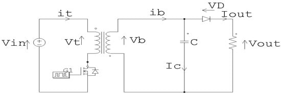
Figure 1.
Electrical scheme of the fly-back converter containing the planar transformer.
Planar transformers come in a variety of forms, depending on the research requirements. The most common forms are as follows: with modified and partially inclined deformed planar windings or with purely planar windings that take the form of part of a sector, the transformer’s primary and secondary. Generally, planar toroidal coils are constructed from two thin coaxial cylinders arranged in parallel. Each cylinder is segmented into n unconnected sectors, leading to gaps between the turns, as shown in Figure 2 [,].
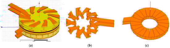
Figure 2.
Example of a transformer with planar toroidal coils: general view (a), primary coil with 20 turns (b), and secondary coil with 10 turns (c).
The coils chosen for the transformer’s primary and secondary are identical and have the following characteristics: number of primary turns nt = 20; number of secondary turns nb = 10; inner diameter din = 37 mm; outer diameter dout = 63 mm; outer diameter of magnetic ferrite material dexNiFe = 60 mm; inner diameter of magnetic ferrite material dinNiFe = 40 mm; outer diameter of PCB material dPCB = 68 mm; turn thickness t = 0.07 mm; and PCB thickness ePCB = 0.3 mm. The electrical characteristics of the toroidal coil, substrate, and insulator are given in Table 1. As is well known, FR4 is a type of fiberglass-reinforced epoxy laminate. It is here used as an insulator.

Table 1.
Characteristics of inductance, substrate, and insulation.
Taking into account certain electrical and magnetic characteristics of the planar transformer, the volume of the magnetic core and the surface area on which the transformer’s electrical circuit will be placed are evaluated. On this basis, the dimensions of the magnetic core can be evaluated while remaining in line with the converter’s specifications in terms of magnetic energy storage and material losses [,].
Our transformer is described geometrically by the following several parameters: the width, the conductor thickness t, the winding spacing s, and the number of turns n, as well as the inside diameter din, the outside diameter dout, and the total conductor length lT, []. The din and dout must be chosen to optimize the ratio between the coil and the surface area occupied on the circuit. This surface is made up of copper conductors laid on three stacked layers, two layers of FR4 and the PCB, between the two layers, and a ferromagnetic layer of NiFe, all laid on a ground plane, as sketched in Figure 3.
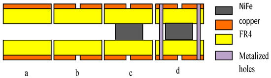
Figure 3.
Process for producing the planar toroidal coil. (a) Thin PCB; (b) etched tracks; (c) magnetic circuit pressed between the two PCBs; and (d) plated through holes to connect the two PCBs.
The following equations can be used to calculate the various geometric parameters:
In Equations (1)–(3), m is the transformation ratio, w is the energy stored in the core, v theenergy density by volume, α represents the duty cycle, Pout is the power at the transformer output, Vin is the input voltage of the transformer, Vout is the voltage at the transformer output, is is the electric current at the output of the transformer, and ie is the electric current at the input of the transformer. The values of the frequency f and the input voltage Vin allow us to calculate the value of the inductances of the primary and secondary coils lt and lb of our transformer. The sizing of the magnetic core is determined by the core volume needed to store the energy, which is calculated using the energy density (as expressed in Equation (3)) and the energy stored in the windings [,]. The volumetric energy that can be stored in the magnetic core wmax is a function both of the maximum induction Bmax that the material can withstand and of its relative permeability µr.
is the thickness of the NiFe. Dout is the outside diameter. We opted for a core section equal to the following:
In conclusion, we found a volume of 314 mm3 of NiFe necessary to store 12.5 µJ of energy. Note that the higher the relative magnetic permeability, the greater the volume of the magnetic circuit will be for a given maximum induction.
The equations below are used to calculate the average width of a single conductor; since its width is not the same, one is greater than the other.
The lengths of the primary and secondary coil conductors can be calculated as follows:
All the parameters involved in the design of the micro-transformer are summarized in Table 2.
Table 2.
Values of transformer’s Geometrical parameter and electrical parameters.
Figure 4 depicts the equivalent electrical model derived from the diagram in Figure 2. This model is utilized to simulate the electrical behavior of the transformer [,], as illustrated in Figure 4. From the three-dimensional cross-section of the transformer, we can deduce the equivalent electrical circuit, as shown in Figure 5.
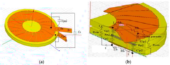
Figure 4.
Schematic of the electrical circuit of the primary inductors (a); parasitic effect between the first and the last turn as well as the inter-turn capacitive effect Cs (b).
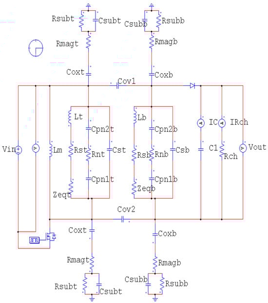
Figure 5.
Model of the equivalent electrical circuit of transformer.
The equivalent electrical model of the transformer is similar to the spiral inductor model, as evident in Figure 5. In fact, the transformer is simply a pair of magnetically coupled spiral inductors. This model includes the series inductances of the primary and secondary coils (lt, lb), the series resistances of the second primary coil (Rst, Rsb), the coupling capacitances between the turns (Cov1,2), the capacitances between the secondary and primary coils and the substrate (Coxt, Coxb), and the substrate capacitance of the primary and secondary coils (Cst, Csb).
Let us now present the analytical expressions for the various elements of the electrical circuit: Rst, Rsb primary and secondary coil substrate resistances; Coxt, Coxb, parasitic capacitance, and oxide capacitors; Cpn2 parasitic capacitance between the part of the core above the last foil at the bottom and the 1st foil at the top (Cpn2 is above Cpn1); Rn2 core resistance; Covt coupling capacitance between turns; and Cst, Csb primary and secondary coil substrate capacitance.
3. Simulating the Magnetic Behavior
Figure 6 shows the influence of the frequency on the inductances of the primary lt and secondary lb. These inductances are extracted from the imaginary part of the impedances and are expressed by Equation (1).
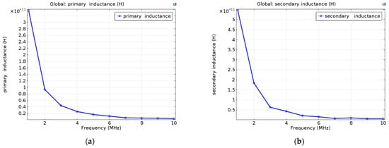
Figure 6.
(a) Influence of the operating frequency on the inductanceprimary (a,b) Influence of the operating frequency on the inductance secondary lb.
Figure 7 shows the influence of the frequency on the series resistors of primary Rst and secondary Rsb. The obtained results are very satisfactory: in fact, the results show that the resistance values increase as the frequency increases and the inductances decrease. Figure 7 shows that the resistances Rst and Rsb increase as a function of frequency (skin effect) and similarly for the impedance (proximity effect). The resistance values are therefore very sensitive to changes in frequency due to the skin and proximity effects. On the other hand, Figure 6 shows that inductance values also vary significantly as a function of frequency. As the frequency increases, skin and proximity phenomena increase. The current density then becomes increasingly inhomogeneous in the conductor, with a concentration on the surface in the skin thickness.
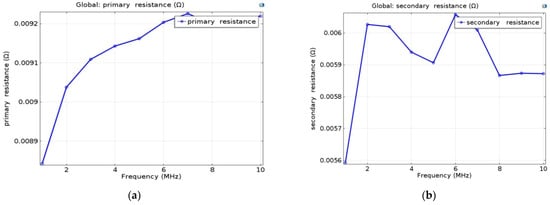
Figure 7.
Behavior ofprimary (a) and secondary (b) series resistance versus frequency.
To visualize the converter output voltage and the output current, we employed PSIM 6.0, a simulation software package for electrical engineering and power electronics; the software allows us to draw the pattern of the mounting from the elements of the library. The expression of fly-back converter load resistance, fly-back converter capacitance and inductance, output power, input power, output power, efficiency, losses Joule, and iron losses are, respectively, given by the following expressions:
Figure 8 reports the appearance of the converter output voltage and current. As expected, these results show that the dimensioning of the transformer was carried out correctly. Indeed, simulation results display input and output voltages of the micro transformer equal to 100 V and 50 V, respectively, with a current Iout = 2 A. These results are in excellent agreement with the specifications.
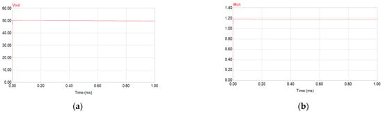
Figure 8.
Output voltage of the integrated transformer (a); output current of the integrated transformer (b).
The specifications are the starting point for sizing the planar transformer. As already discussed, the transformer consists of two planar toroidal coils deposited on a magnetic material and separated by a dielectric, which also provides the magnetic coupling, as sketched in Figure 9.
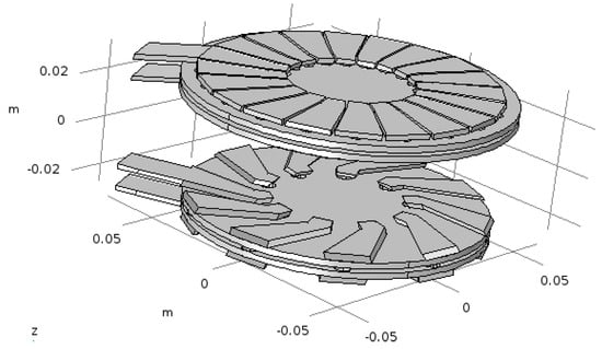
Figure 9.
View in 3D of the primary and secondary transformer.
The electromagnetic phenomenon is governed by Maxwell’s equations:
The numerical resolution of the physical problem for the study of the magnetothermal behavior of the transformer was carried out using the finite element method based on Galerkin discretization under the software package COMSOL Multiphysics 6.0. The solution of Equation (12) will allow us to visualize the magnetic behavior of the planar coil [,]. Figure 10 illustrates the mesh grid adapted to the device object of the present analysis.It is a tetrahedral grid refined in the vicinity of the walls of the study area, including the transformer boundaries. In order to ensure the reliability and accuracy of the numerical results, a test of the independence of the results with respect to the type of mesh and the number of elements was carried out. For this purpose, we opted for a number of elements of 1,235,802, beyond which the simulation results remain unchanged.
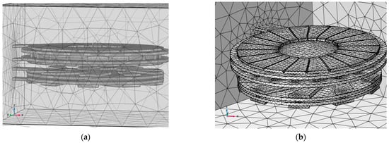
Figure 10.
Mesh size of the study area (a). Mesh size of the transformer (b).
To provide a more detailed analysis, two cases have been studied: a coil with a magnetic core and without a magnetic core. In this framework, Figure 11 shows the distribution of the electrical potential across the turns of the toroidal coils in both cases. In both cases, it can be seen that the potential is greater in the primary winding than in the secondary winding. This is because this type of transformer is a step-down transformer. On the other hand, through the primary and secondary windings, the electrical potential gradually decreases between the inputs and outputs of the coils. Moreover, the electrical potential is almost identical between the two cases. In addition, the input current decreases along the turns of the transformer due to the resistance of the conductor.
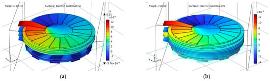
Figure 11.
Distribution of electrical potential in the transformer: without NiFe (a) with NiFe (b).
Figure 12 shows the magnetic flux density produced by the transformer in the two cases studied. We can see that the magnetic flux density generated by the transformer with the magnetic core is the greatest.
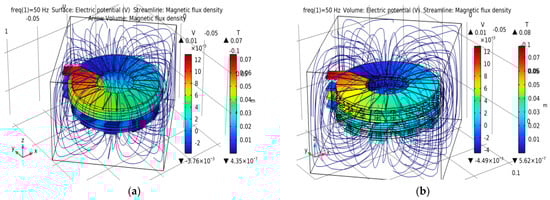
Figure 12.
Distribution of the magnetic flux density in the transformer: without NiFe (a); with NiFe (b).
For a more detailed analysis, Figure 13 shows the magnetic flux density distribution along the vertical line running through the middle of the transformer’s two coils. It can also be seen that the magnetic density generated by the transformer is greater when a magnetic core is present. This confines the magnetic field lines, leading to a peak at the magnetic core.
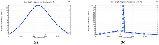
Figure 13.
Distribution of the magnetic flux density distribution in the transformer along the vertical central line: without NiFe (a); with NiFe (b).
By solving Maxwell’s equations, we can also visualize the electrical current density distribution in the planar toroidal transformer in 3D. Figure 14 shows the current density distribution in the planar transformer. It is minimal inside the transformer because of the conductor resistance. Moreover, it is not uniform in the planar transformer; it is greater at the corners, which induces non-homogeneous resistance in the conductors []. It should be noted that the skin effect and the proximity effect are present and occur, in particular, between adjacent conductors. Figure 15 shows the distribution of the electric current density in the two toroidal coils making up our transformer in the two cases: absence and presence of a magnetic material (a magnetic core). By virtue of the homogeneity of the coil material, the current density in both cases is the same. On the other hand, in both cases, the current density is high at the links connecting the upper and lower turns. This is due to the small cross-section of the links.
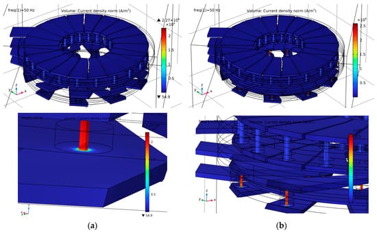
Figure 14.
Distribution of current density on the turns of the coils forming the transformer, with detail immediately above: without NiFe (a); with NiFe (b).
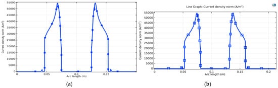
Figure 15.
Distribution of current density along a direction passing through the expanded primary and secondary turns: without NiFe (a); with NiFe (b).
As shown in Figure 16, indeed, across a horizontal line that passes longitudinally through two primary windings facing each other in the two cases studied, the current density curves are almost identical. On the other hand, along the measurement line, the current density increases as the turn shrinks (from the outside diameter to the inside diameter).
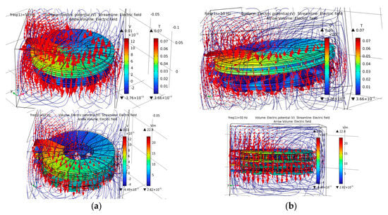
Figure 16.
Distribution of the electric field in the study area from different perspectives: without NiFe (a); with NiFe (b).
Let us now investigate the electric field. Figure 16 shows the distribution of the electric field lines in the vicinity of the coil in both cases. As is recognized in the literature, the electric field has a divergent pattern perpendicular to the surface of the coils. On the other hand, by comparing the two cases studied, we can see that the electric field intensity is lower in the presence of a magnetic core, as evident in Figure 17.
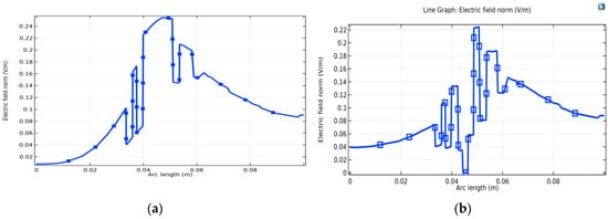
Figure 17.
Electric field distribution along a direction passing through the expanded primary and secondary turns: without NiFe (a); with NiFe (b).
4. Thermal Behavior of the Planar Transformer
A complete sizing of the transformer requires a study of its thermal behavior. In most cases, an increase in temperature can lead to severe degradation of the equipment, reducing its lifespan or even putting it out of service. In this section, we will present a study of the thermal behavior of the toroidal winding transformer using a mathematical model that is a coupling between Maxwell’s equations and the heat equation in the following two cases: windings with and without a magnetic core.
Equation (13) is used to determine the temperature distribution in a given area, taking into account the different transmission modes [,,,,,].
In Equation (13), p represents the source term due to an internal heat generation [W/m3], and the subscript i corresponds to the nature of the material: copper, PCB, or air. Moreover, T is the temperature [K], is the speed of the air if it is in motion (convection) [m/s], t is time [s], is the density of the material [Kg/m3], Cp is the heat capacity of the material [J/(Kg K)], and λ is the thermal conductivity of the material [W/(m K)].
Our thermal study is performed in 3D, which allows us to transcribe Equation (14) in general writing. By posing and , one obtains the following:
Moreover, in the hypothesis of negligible convection, Indeed,
Moreover, let us assume material homogeneity, i.e., (constants). Then,
In the steady case, one has
where the source term p corresponds to the heat flux released by the conductor by the Joule effect:
P = RI2
By substituting the resistance expression, one has the following:
Indeed, the equation to be solved is
The general conditions of the simulation are as follows: The isotropy of the different materials in the study domain, the thermal conductivity coefficient, depends on the temperature, and the thermal convection is introduced as a condition at the boundaries of the planar substrate–coil assembly. The micro-coil is a heat source, and its term is well introduced in Equation (15). At time t = 0, the temperature of the coil, substrate, and air is considered to be at room temperature, 20 °C. At the boundaries of the air box, the convective flux is given by the following:
In Equation (15), is the air conductivity [W/mK)], is the direction normal to the border [m], is the air convection coefficient [W/(m2 K)], and is the ambient temperature.
5. The Thermal Behavior
In this section, we present a comparison between the thermal behavior of our devices in the presence and absence of a magnetic core. Figure 18 and Figure 19 illustrate the temperature distribution within the study area. We can see that the highest temperature is at the secondary coil turns in both cases. On the other hand, the greatest amount of heat was generated by the transformer, which does not have a magnetic core. At the turns of the two transformers, the temperature rises as the electric current moves away from the outlets and inlets. On the other hand, the temperature peak is located at the cylindrical links connecting the upper and lower turns. The small diameter of these links results in a high current density, leading to an increase in temperature.
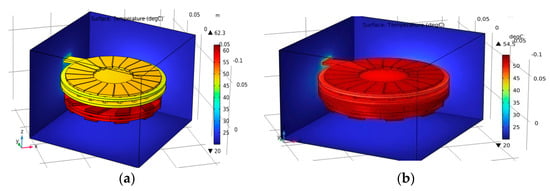
Figure 18.
Temperature distribution in the global simulation domain: without NiFe (a); with NiFe (b).
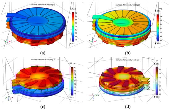
Figure 19.
Temperature distribution in the primary coils: Distribution of the electric field in the study area from different perspectives: without NiFe (a); with NiFe (b), and in the secondary coils: without NiFe (c); with NiFe (d).
Figure 20 shows the temperature distribution along the vertical median line crossing the study area in the presence and absence of a magnetic core. The thermal behavior of the system changes radically with the introduction of this core. Without the core, the temperature is higher, particularly in the vicinity of the coils. With the introduction of the magnetic core, the temperature becomes lower by changing its distribution structure. The lower temperature is due to the higher thermal conductivity of the ferrite, which dissipates more heat.
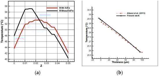
Figure 20.
Validation: thermal distribution along the vertical center line with and without magnetic core (a); temperature distribution in the core and comparison with the literature (b).
In order to ensure the reliability of our numerical results, we first compared one of our results with that available in the literature [], by putting us in the same conditions of simulation. Figure 20 displays the temperature distribution in the study area. It appears clearly that there is a great agreement between our results, which validates our model.
6. Conclusions
The present analysis concerns the study of the magnetothermal behavior of a toroidal transformer intended to be inserted into a fly-back converter. Indeed, the latter is increasingly used in low- and very-low-power electronic devices because it presents major interests in terms of size, efficiency, and manufacturing. The paper deals with optimizing the operation of this transformer by studying the two phenomena to which it is subject: its magnetic and thermal behavior. To carry out this study, we first had to carry out a sizing, which allowed us to determine the different geometric and electrical parameters characterizing this transformer. The study of magnetothermal behavior using mathematical models describing these phenomena and the resolution of the governing equations has shown the distribution of currents and voltages, the magnetic field, as well as the distribution of temperature in the different layers. of materials making up this transformer. All these results made it possible to identify the optimal operation of this transformer.
Author Contributions
Conceptualization, K.B., A.H., E.R.d.S., A.M., R.M. and P.V.; methodology, E.R.d.S., A.M. and P.V.; software and validation K.B., A.H., A.M. and R.M.; investigation, K.B., A.H., E.R.d.S., A.M., R.M. and P.V.; writing—original draft preparation, K.B., A.H., E.R.d.S., A.M. and R.M.; writing—review and editing, K.B., A.H., E.R.d.S., A.M., R.M. and P.V.; visualization, K.B., A.H., A.M. and R.M.; supervision, E.R.d.S., A.M. and P.V. All authors have read and agreed to the published version of the manuscript.
Funding
This research received no external funding.
Data Availability Statement
The original contributions presented in the study are included in the article, further inquiries can be directed to the corresponding author.
Conflicts of Interest
The authors declare no conflicts of interest.
References
- Benzidane, M.R.; Melati, R.; Benyamina, M.; Meskine, S.; Spiteri, P.; Boukortt, A.; Adda Benattia, T. Miniaturization and optimization of a DC–DC boost converter for photovoltaic application by designing an integrated dual-layer inductor model. Trans. Electr. Electron. Mater. 2022, 23, 462–475. [Google Scholar] [CrossRef]
- Luna, M. High-Efficiency and High-Performance Power Electronics for Power Grids and Electrical Drives. Energies 2022, 15, 5844. [Google Scholar] [CrossRef]
- Raghavendra, K.V.G.; Zeb, K.; Muthusamy, A.; Krishna, T.N.V.; Kumar, S.V.P.; Kim, D.H.; Kim, M.S.; Cho, H.G.; Kim, H.J. A comprehensive review of DC–DC converter topologies and modulation strategies with recent advances in solar photovoltaic systems. Electronics 2019, 9, 31. [Google Scholar] [CrossRef]
- Aggas, J.M. Planar Magnetics Design for Low Voltage High Power DC-DC Converters. Doctoral Dissertation, Auburn University, Auburn, AL, USA, 2014. [Google Scholar]
- Bose, B.K. Global energy scenario and impact of power electronics in 21st century. IEEE Trans. Ind. Electron. 2012, 60, 2638–2651. [Google Scholar] [CrossRef]
- Melati, R.; Hamid, A.; Thierry, L.; Derkaoui, M. Design of a new electrical model of a ferromagnetic planar inductor for its integration in a micro-converter. Math. Comput. Model. 2013, 57, 200–227. [Google Scholar] [CrossRef]
- Derkaoui, M.D.M.; Hamid, A.; Lebey, T.L.T.; Melati, R. Design and modeling of an integrated micro-transformer in a flyback converter. IEEE Trans. Power Electron. 2013, 11, 669–682. [Google Scholar] [CrossRef][Green Version]
- Li, Q.; Wolfs, P. A review of the single phase photovoltaic module integrated converter topologies with three different DC link configurations. IEEE Trans. Power Electron. 2008, 23, 1320–1333. [Google Scholar]
- Shawky, A.; Ahmed, M.; Orabi, M.; Aroudi, A.E. Classification of three-phase grid-tied microinverters in photovoltaic applications. Energies 2020, 13, 2929. [Google Scholar] [CrossRef]
- Liu, Y.; Liu, X.; Lu, Q.; Zhang, T.; Yin, X. A T-model with parameter extraction method for modeling 3-D spiral inductor. IEEE Microw. Wirel. Compon. Lett. 2021, 32, 37–40. [Google Scholar] [CrossRef]
- Kouril, L.; Pospisilik, M.; Adamek, M.; Jasek, R. Coil optimization with aid of flat coil optimizer. In Proceedings of the 5th WSEAS Congress on Applied Computing Conference, and Proceedings of the 1st International Conference on Biologically Inspired Computation. World Scientific and Engineering Academy and Society (WSEAS), Faro, Portugal, 2–4 May 2012. [Google Scholar]
- Senhadji, N.; Hamid, A.; Bley, V.; Leby, T. Design and integration of planar inductances on PCB application passive type filters. Trans. Electr. Electron. Mater. 2020, 21, 123–137. [Google Scholar] [CrossRef]
- Derkaoui, M.; Benhadda, Y.; Hamid, A. Modeling and simulation of an integrated octagonal planar transformer for RF systems. SN Appl. Sci. 2020, 2, 656. [Google Scholar] [CrossRef]
- Ferrell, J.; Lai, J.S.; Nergaard, T.; Huang, X.; Zhu, L.; Davis, R. The role of parasitic inductance in high-power planar transformer design and converter integration. In Proceedings of the Nineteenth Annual IEEE Applied Power Electronics Conference and Exposition, 2004, APEC’04, Anaheim, CA, USA, 22–26 February 2004; Volume 1, pp. 510–515. [Google Scholar]
- Wang, S.; Xu, C. Design theory and implementation of a planar EMI filter based on annular integrated inductor–capacitor unit. IEEE Trans. Power Electron. 2012, 28, 1167–1176. [Google Scholar] [CrossRef]
- Yunas, J.; Majlis, B.Y. Comparative study of stack interwinding micro-transformers on silicon monolithic. Microelectron. J. 2008, 39, 1564–1567. [Google Scholar] [CrossRef]
- Zhang, Y.; Li, E.; Long, H.; Feng, Z. Accurate model for micromachined microwave planar spiral inductors. Int. J. RF Microw. Comput.-Aided Eng. 2003, 13, 229–238. [Google Scholar] [CrossRef]
- Lewaiter, A.; Ackermann, B. A thermal model for planar transformers. In Proceedings of the 4th IEEE International Conference on Power Electronics and Drive Systems, IEEEPEDS2001-Indonesia, Proceedings (Cat. No. 01TH8594), Denpasar, Indonesia, 25–25 October 2001; IEEE: Piscataway, NJ, USA, 2001; Volume 2, pp. 669–673. [Google Scholar]
- Allaoui, A.; Hamid, A.; Spitéri, P.; Bley, V.; Lebey, T. Thermal modeling of an integrated inductor in a micro-converter. J. LowPower Electron. 2015, 11, 63–73. [Google Scholar] [CrossRef]
- Benhadda, Y.; Hamid, A.; Lebey, T. Thermal modeling of an integrated circular inductor. J. Nano Electron. 2017, 9, 1004. [Google Scholar] [CrossRef]
- Hu, J. Analyses of the temperature field in a bar-shaped piezoelectric transformer operating in longitudinal vibration mode. IEEE Trans. Ultrason. Ferroelectr. Freq. Control 2003, 50, 594–600. [Google Scholar]
- Joo, H.W.; Lee, C.H.; Rho, J.S.; Jung, H.K. Analysis of temperature rise for piezoelectric transformer using finite-element method. IEEE Trans. Ultrason. Ferroelectr. Freq. Control 2006, 53, 1449–1457. [Google Scholar] [CrossRef]
- Susa, D.; Lehtonen, M.; Nordman, H. Dynamic thermal modelling of power transformers. IEEE Trans. Power Deliv. 2005, 20, 197–204. [Google Scholar] [CrossRef]
- Rajnak, M.; Wu, Z.; Dolnik, B.; Paulovicova, K.; Tothova, J.; Cimbala, R.; Timko, M. Magnetic field effect on thermal, dielectric, and viscous properties of a transformer oil-based magnetic nanofluid. Energies 2019, 12, 4532. [Google Scholar] [CrossRef]
- Benhadda, Y.; Derkaoui, M.; Kharbouch, H.; Hamid, A.; Spiteri, P. Numerical Simulation for Cooling of Integrated Toroidal Octagonal Inductor Using Nanofluid in a Microchannel Heat Sink. Metall. Mater. Eng. 2024, 30, 17–44. [Google Scholar] [CrossRef]
- Mokhefi, A.; Rossi di Schio, E. Effect of a magnetic field on the Couette forced convection of a Buongiorno’s nanofluid over an embedded cavity. JP J. Heat Mass Transf. 2022, 30, 89–104. [Google Scholar] [CrossRef]
- Caillaud, R.; Buttay, C.; Mrad, R.; Le Lesle, J.; Morel, F.; Degrenne, N.; Mollov, S. Comparison of planar and Toroidal PCB integrated inductors for a multi-cellular 3.3 kW PFC. In Proceedings of the 2017 IEEE International Workshop on Integrated Power Packaging (IWIPP), Delft, The Netherlands, 5–7 April 2017; pp. 1–5. [Google Scholar]
- Pasko, S.W.; Kazimierczuk, M.K.; Grzesik, B. Self-capacitance of coupled toroidal inductors for EMI filters. IEEE Trans. Electromagn. Compat. 2015, 57, 216–223. [Google Scholar] [CrossRef]
- Wheeler, H.A. Simple inductance formulas for radio coils. Proc. Inst. Radio 1928, 16, 1398–1400. [Google Scholar] [CrossRef]
- Mohan, S.S.; del Mar Hershenson, M.; Boyd, S.P.; Lee, T.H. Simple accurate expressions for planar spiral inductances. IEEE J. Solid-State Circuits 1999, 34, 1419–1424. [Google Scholar] [CrossRef]
Disclaimer/Publisher’s Note: The statements, opinions and data contained in all publications are solely those of the individual author(s) and contributor(s) and not of MDPI and/or the editor(s). MDPI and/or the editor(s) disclaim responsibility for any injury to people or property resulting from any ideas, methods, instructions or products referred to in the content. |
© 2024 by the authors. Licensee MDPI, Basel, Switzerland. This article is an open access article distributed under the terms and conditions of the Creative Commons Attribution (CC BY) license (https://creativecommons.org/licenses/by/4.0/).