Abstract
Aiming at the problem of source-load uncertainty caused by the increasing penetration of renewable energy and the large-scale integration of electric vehicles (EVs) into modern power system, a robust optimal operation scheduling algorithm for regional integrated energy systems (RIESs) with such uncertain situations is urgently needed. Based on this background, aiming at the problem of the irregular charging demand of EV, this paper first proposes an EV charging demand model based on the trip chain theory. Secondly, a multi-RIES optimization operation model including a shared energy storage station (SESS) and integrated demand response (IDR) is established. Aiming at the uncertainty problem of renewable energy, this paper transforms this kind of problem into a dynamic robust optimization with time-varying parameters and proposes an improved robust optimization over time (ROOT) algorithm based on the scenario method and establishes an optimal scheduling mode with the minimum daily operation cost of a multi-regional integrated energy system. Finally, the proposed uncertainty analysis method is verified by an example of multi-RIES. The simulation results show that in the case of the improved ROOT proposed in this paper to solve the robust solution of renewable energy, compared with the traditional charging load demand that regards the EVs as a whole, the EV charging load demand based on the trip chain can reduce the cost of EV charging by 3.5% and the operating cost of the multi-RIES by 11.7%. With the increasing number of EVs, the choice of the starting point of the future EV trip chain is more variable, and the choice of charging methods is more abundant. Therefore, modeling the charging demand of EVs under more complex trip chains is the work that needs to be studied in the future.
1. Introduction
In the face of increasingly serious energy and environmental problems, building an energy-sustainable and environmentally friendly development strategy is a key issue of common concern in the world today [1,2]. A regional integrated energy system (RIES), which is based on a renewable energy source (RES) and combined cooling heating and power (CCHP), can improve energy efficiency due to its complementary characteristics between energy sources and energy ladder utilization characteristics [3,4]. However, with the increasing penetration of RES and the massive access of electric vehicles (EVs) as loads to RIES, the RIES faces more uncertainties due to the RES’s inherent randomness and volatility and EVs’ irregular charging time and charging power. Based on the above background, it is of great theoretical and practical significance to study the RIES optimal scheduling method considering the uncertainty of RESs and EVs [5].
Large-scale EV access to a power grid will bring problems such as increased network loss and decreased power quality to the power grid [6]. In reference [7], a model considering advanced support vector machine (SVM) and hybrid electric vehicle (EV) charging demand is proposed, and the influence of hybrid EV charging on the whole system is studied. Considering the dual attributes of EVs with load and energy storage equipment, reference [8,9] proposed that the orderly participation of EVs in grid activities can reduce the load peak–valley gap and improve the scheduling flexibility. Reference [10] proposes that EVs, as a flexible energy storage carrier, can smooth the energy fluctuations caused by the uncertainty of RESs, and through the guidance of electricity price, EVs can improve the consumption rate of the RES to a certain extent. For the coordinated scheduling problem of EVs in integrated energy system, reference [11] proposed an EV charging behavior framework based on time-of-use (TOU) electricity price guidance to attract EVs users to charge during the valley price period. On the basis of the TOU electricity price, reference [12] proposes that when the load is at the peak, the EVs can be used as a power source to discharge to the system to a smooth load curve. Example results show that a certain scale of EVs can be used as a backup power source to alleviate the system operating pressure during peak periods. Reference [13] also proposes a decentralized EV scheduling strategy based on the TOU electricity price. In reference [14], an optimization model with the objective of minimizing household energy consumption is established for EV home users with self-use energy storage equipment. Experimental results show that the reasonable use of EV charging and discharging can reduce the cost of energy consumption. However, most of the current research only focuses on the charging and discharging behavior of an EV at a fixed time of place and does not fully consider the characteristics of the non-fixed-time random charging of an EV during use, which is very common in the use of EV.
Due to the unpredictability of the natural environment in which RES equipment is located, there is a high uncertainty in RES output, which is one of the main reasons for the uncertainty of the power supply side. In order to solve the uncertainty of RES, reference [15] proposed a prediction method based on a deep learning approach (DLA) from the perspective of prediction. Reference [16] by assigning the probability to chance constraint of each constraint event, the complex combinatorial chance constraint is transformed into a severalty chance constraint for solution. Reference [17] uses the method of support vector machine to identify zero-probability events, improve the average distribution of intersection probability, and improve the reliability of the consequences. In reference [18], an algorithm based on Wasserstein Gan with gradient penalty (WGAN-GP) is proposed to delineate the scenarios of renewable energy. In reference [19], the uncertainty problem is modeled by improving the generative adversarial network. In reference [20], they propose a two-stage distributed robust optimization algorithm and integrate a data-driven approach to deal with these uncertainty problems. In reference [21], a two-stage model is established to solve the uncertainty of a RES and the economy of power grid operation, and experimental results show that this model can achieve system robustness while reducing operating costs.
At present, most of the research on the charging behavior of an EV connected to the power grid regards the EV as a whole part and conducts charging and discharging behavior at a fixed time, while ignoring the randomness of the individual charging behavior of the EV; meanwhile, most of the research on the uncertainty of RESs based on scenario method does not consider whether data after scenario reduction are robust. Aiming at these problems in current research, in this paper, the charging demand model of EV is established based on the trip chain theory, and an improved robust optimization over time (ROOT) algorithm based on the scenario method is proposed to solve the uncertainty problem of RESs. The main contributions are as follows:
- Aimed at the randomness of EV charging behavior, a charging demand model of an EV based on trip chain theory is proposed;
- Aimed at the RES uncertainty problem, an improved robust optimization over time algorithm based on the scenario method is proposed;
- Based on the existing comprehensive demand response, a cold–heat–electric alternative integrated demand response (IDR) model is proposed.
The rest of this paper is structured as follows. Section 2 introduces the basic structure of the RIES, IDR and shared energy storage station (SESS). In Section 3, the EV charging demand model based on the trip chain theory is established. In Section 4, the algorithm for solving the uncertainty of RES is proposed. In Section 5, the optimization model is established. Section 6 presents example analysis and finally, the conclusions are given in Section 7.
2. Structure Modeling of RIES Based on SESS and IDR
2.1. Overall Framework of RIES
The structure of RIES is shown in Figure 1. It is known from Figure 1 that the RIES includes several CCHPs in different regions, and each CCHP is connected to the external power network, gas network and water network. Each CCHP provides cold, heat and electricity energy supply for their respective energy users. At the same time, a power transmission node is established at each CCHP, which is connected to the SESS through the node. Because there is no direct electrical interaction between each CCHP in this region, CCHP can only interact with the external power grid (EPG) or SESS through the power network.

Figure 1.
The structure of RIES with SESS.
For any CCHP shown in Figure 1, its internal structure is shown in Figure 2. It is known from Figure 2 that CCHP is mainly composed of the following components: energy supply, energy conversion, energy demand and energy exchange. The energy supply part comprises a wind turbine (WT), photovoltaic (PV), gas turbine (GT) and gas boiler (GB), and EPG, which is connected to the CCHP via a transformer. The energy conversion part comprises a waste heat boiler (WHB), electric boiler (EB), absorption chiller (AC), heat exchanger (HE), electrical chiller (EC) and electric storage (ES). The energy demand part comprises electrical, cooling and heating loads. The energy exchange part mainly comprises the SESS, EV, other CCHPs, external energy market and carbon market, etc. The CCHP receives the natural gas and the electric energy provided by the EPG and RES included in the energy supply and converts it into the energy needed by the user through the energy coupling device of the energy conversion, and finally provides it to the energy demand. At the same time, the CCHP also participates in other forms of energy interaction mentioned in the energy exchange. This paper mainly studies the interaction between the CCHP, EV and SESS. The detailed modeling work of the equipment in CCHP can be found in reference [22], which will not be introduced in this paper.

Figure 2.
The structure of the CCHP.
2.2. Modeling of SESS
An SESS usually refers to a model in which a public energy storage device provides energy storage services to multiple users [23,24]. An SESS utilizes the difference and complementarity of load curves of different users, and through the integration and optimization, to improve the utilization of energy storage equipment, the level of RES consumption and the user’s benefit, so as to realize value creation [25,26,27]. An SESS should satisfy the following constraints.
2.2.1. Power Continuity Constraint
Under the action of the user’s charging and discharging behavior, the internal energy of SESS should remain continuous.
where and are the state of charge (SOC) of the SESS at time and , respectively; and are the charge and discharge power at time , respectively; , and are the self-discharge, charge and discharge efficiency, respectively; and is the scheduling time interval.
2.2.2. SOC Constraints
The SOC of SESS cannot exceed the design parameters of its equipment.
where , and are the maximum, initial and final SOC of the SESS, respectively; , and are the lower limit, upper limit and initial coefficient of the SOC, respectively.
2.2.3. Charge and Discharge Constraints
There can be no simultaneous charging and discharging behavior between the SESS and the user.
where is the maximum power of the SESS; and are the charging and discharging state bits of the SESS at time , respectively.
2.3. Modeling of IDR
An IDR is an important means of RIES load demand management [28]. It aims to guide power users and load aggregators to adjust energy consumption strategies through market-oriented means, actively participate in power grid valley filling, and improve the reliability of power system operation. This paper divides the IDR load into a reducible load (RL), transferable load (TL) and substituted load (SL).
2.3.1. Modeling of RL
Energy users determine whether the current load is a RL by comparing the changes in energy prices during the scheduling period. RL can be described as follows:
where is the variation in RL after IDR; is the initial RL; is the price elasticity matrix of the RL; is the energy price at time ; and is the initial energy price at time .
The constraint of RL is as follows:
where is the maximum value of .
2.3.2. Modeling of TL
TL refers to those loads the access time of which users can flexibly adjust according to their demand price. The TOU energy price is used as the signal to guide users to transfer the load from the peak price period to valley price period. TL can be described as follows:
where is the variation in the TL after IDR; is the initial TL; is the price elasticity matrix of the TL.
The constraint of the TL is as follows:
where is the maximum value of .
2.3.3. Modeling of SL
For those loads that can be directly supplied by electric energy or cold/heat energy, when the electricity price per unit of energy supply is less than the price of cold/heat energy, electric energy is used to substitute cold/heat energy; otherwise, cold/heat energy is used to substitute electric energy. SL can be described as follows:
where and are the substituted electrical load and corresponding substituted cold/heat load, respectively; is the electro-cold/heat substitution coefficient; and are unit calorific values of electric and cold/heat, respectively; and and are the energy efficiency of electric and cold/heat, respectively.
The constraints of SL are as follows:
where and are the minimum and maximum substitution values of the substituted electrical load, respectively; and are the minimum and maximum substitution values of the substituted cold/heat load.
3. EV Modeling Based on Trip Chain Theory
3.1. Basic Theory of EV Trip Chain
The trip chain simulates a series of behavioral characteristics during the period from the initial point to the terminal point [29]. The EV trip chain is defined as a space–time chain formed by linking the time series and spatial state of the EV travel process, with the residence of the EV user as the starting point and terminal point. Figure 3 is the schematic diagram of the EV trip chain.

Figure 3.
Schematic diagram of the EV trip chain.
The variables describing the spatial transfer of EV are called spatial variables, including destination and driving distance . The variables describing the change in the EV driving and stopping state are called time variables, including the start time of driving , end time of driving , driving time and parking time .
Based on the actual EV usage environment, it is known that EV travel behavior has the memoryless nature of Markov chains. That is, the destination of an EV driving at time is only related to the last driving destination , and is not related to any of the travel destinations . Based on this fact, the trip chain of EV can be regarded as a special class of Markov chain. The state of an EV at time is , and the state at the next moment is . According to the Markov chain theory, the probability from to is as follows:
where is the probability of EV transferring from the current state to the next state. Based on (1), the space transition probability matrix of EV can be expressed as follows:
In order to construct a reasonable EV trip chain, based on the data of the national household travel survey (NHTS), the NHTS divides the parking places of vehicles within one day into three types: home, work and other, and according to the data of the NHTS, the probability of EV in different parking places at the initial state () is shown in Table 1.

Table 1.
The probability of an EV in a different parking place at the initial state.
3.2. Modeling of EV Trip Chain
According to the trip chain theory, the following models can be established. The probability distribution function (PDF) of is shown as follows:
where and are the mathematical expectation of and variance in PDF, respectively.
The obeys the normal distribution, and its PDF is as follows:
The can be calculated by driving time and average speed . The average driving speed is affected by many factors, such as real-time traffic conditions. According to <China’s major urban traffic analysis report>, the average speed of automobiles in Lanzhou is 35.17 km/h. Similarly, can be obtained by summing and .
The PDF of the home area parking time , working area parking time and other area parking time are shown as follows:
- The PDF of the home area parking time:
- The PDF of the working area parking time:
- The PDF of the other area parking time:
The spatial variable is determined by the actual engineering application environment, and the time variable is obtained by (12)~(16). Based on the above data, a complete EV trip chain can be constructed to obtain the EV charging load demand of each charging station in a scheduling day.
4. Uncertainty Analysis of Renewable Energy Based on Scenario Method and Improved Robust Optimization over Time
In the actual engineering environment, there are many uncertain factors affecting RES. Therefore, from the perspective of cybernetics, this paper regarded a WT and PV as a kind of time-varying factor, transformed the uncertainty of an RES into a kind of dynamic optimization problem with time-varying parameters, and focused on the robustness of output data in the time domain. ROOT is a new algorithm for solving dynamic optimization problems with time-varying parameters. Its central idea is to find a time–domain robust solution and make the solution applicable to a variety of changing environments to improve the stability and robustness of the system operation. Therefore, the ROOT algorithm is more feasible than the traditional optimization algorithm in practical engineering problems [30,31]. At the same time, this paper used the Latin hypercube sampling (LHS) and backward reduction (BR) scenario method as a pre-method to establish the renewable energy output curve, which can make the time-varying factors transformed by the wind power output curve and the photovoltaic processing curve contained in the established dynamic optimization problem as close as possible to the actual output of renewable energy and obtain a more realistic time–domain robust solution.
4.1. Scene Analysis Method
The scene analysis method mainly includes two parts: scene generation and scene reduction. Scene generation refers to the large-scale scenarios with uncertain characteristics obtained by sampling according to the PDF or statistical characteristics of the research object, which can be represented by the set . In this paper, LHS was used as a method for scene generation. Scene reduction reduces the number of similar scenes by analyzing the data set of set , obtains the expected number of scenes, and reduces computational complexity. In this paper, BR was used as a method for scene reduction. The set , composed of a small number of classical scenes, was obtained by BR, which can represent the random variables of the original scene to a large extent. The process is shown in Figure 4.

Figure 4.
Process of scenario analysis.
4.1.1. Scene Generation Based on LHS
LHS can divide a large interval into several fixed intervals, generates a probability value in each interval , then reorders the intervals according to the probability value of each interval. LHS was used to sample multiple renewable uncertain data at the hourly level, and the sample set was constructed by using sampling results.
4.1.2. Scene Reduction Based on BR
In order to merge the similar scenes more effectively, a scene reduction model based on BR was constructed to process the large amount data. We defined the stochastic scenario , where is the reduced object at time in m-th scene; then, we defined the probability of the occurrence of scenario as . The distance between and can be described as follows:
The objective of BR is to minimize the probabilistic distance between the set of scenes before reduction and the set of scenes retained after reduction, which can be described as follows:
where is the set of deleted scenes for scene reduction.
4.1.3. Curving Fitting
According to the number of scenarios obtained from the scenario reduction and probability of occurrence of the corresponding scenarios , it is possible to calculate optimal RES output fitting curve , which can be described as follows:
where is the number of scenes after scene reduction, which is specified by the decision maker. Then, we could fit curve , and the algebraic expression could be obtained. The specific steps of the scene analysis method proposed in this paper are shown in Figure 5.

Figure 5.
The specific steps of scenario analysis.
4.2. Uncertainty Analysis of Renewable Energy Based on the Scenario Method and Improved Robust Optimization over Time
4.2.1. Description of Renewable Uncertainty Problem
The optimal scheduling result of the RIES is based on the establishment of robustness, and robustness requires RIES to be able to maintain stability under different operating environments. Therefore, this paper considered predicting the minimum output of the RES. According to the fitting curve of RES output obtained by LHS and BR, the optimization problem with time-varying parameters was established as follows:
where is the output of renewable generation; is the objective function; and and are the output of the WT and PV, respectively, and are both time-varying parameters. Suppose that and are constants that remain constant, and each change only occurs at the scheduling time point. That is, in a fixed period of time , the optimization problem described by (17) can be re-formulated as follows: with the change in parameters and , it is divided into a sequence of functions composed of multiple static functions. These can be described as follows:
From the above analysis, it can be seen that for the dynamic optimization problem with time-varying parameters shown in (21), ROOT has good engineering application value because it can find the robust solutions of the time-varying elements of the WT and PV in the time domain of the dynamic optimization problem. Therefore, ROOT was introduced to solve the problem. However, most ROOT algorithms need to use future predicted fitness values to find solutions with better robustness. However, the existing methods ignore the influence of prediction error on the robustness of the solution, and the prediction error is large, so it is difficult to find a better robust solution. In order to reduce the influence of prediction error on the robustness of the solution, this paper makes full use of the change trend of the fitness value of the solution in the historical moment and the future moment and guides the algorithm to select the better solution of survival time (ST) and average fitness (AF) [32] in the solution space. At the same time, by analyzing the characteristic quantity of the change in the fitness value of the solution, the limitation of the prediction error on the robustness optimization is reduced.
4.2.2. Improved ROOT
This paper introduces two new evaluation metrics: feasible direction (FD) and stability degree (SD), to reduce the influence of the error of predicted value on the robustness evaluation of ROOT solution. Based on these new evaluation metrics, a ROOT based on the characteristics change in fitness value (ROOT-CCFV) was proposed, so that the optimal solution obtained by ROOT-CCFV could have better robustness in multiple dynamic environments.
- Feasible direction
The FD is used to describe the change trend of function.
where is the decision variable, is the current moment; is the number of historical environments; is the number of future environments; and is the time-varying parameter. The magnitude of FD is proportional to the change in objective function value: a large FD indicates that current objection function value changes with more magnitude at that moment.
- Stability degree
The SD is used to describe the stability of the predicted value.
where is the fluctuation threshold. When the SD is positive, it means that the objective function of the solution in the current environment is not smaller than the mean value curve of the known objective function.
- ROOT-CCFV
In ROOT-CCFV, the FD and SD of the solutions are firstly judged, and the better solution is selected, then the robustness of the selected solutions is evaluated by ST and AF, and finally the optimal robust solution satisfying the actual requirements is obtained. The algorithm flow based on scenario method and ROOT-CCFV is shown in Figure 6.

Figure 6.
Process of ROOT-CCFV based on the scenario method.
5. Optimal Scheduling Model Considering EV and Renewable Energy Uncertainty
5.1. Optimization Objective
The objective functions are expressed as follows:
where and are the electrical energy transaction expenditure and gas energy transaction expenditure with EPG, respectively; is the operation and maintenance expenditure of RIES; and is the energy transaction expenditure with SESS.
where is the number of CCHP; is the CCHP; is the length of the scheduling period; is the time period ; is the purchase price of electricity energy from the EPG; is the purchase power of electricity; is the price of electricity energy sold to the EPG; and is the sale power of electricity.
where is the price of natural gas; and are the electrical and heat power output of the GT and GB, respectively; and are the efficiencies of the GT and GB, respectively; and is the heating value of natural gas.
where , and are the operating and maintenance expenditure of electric energy equipment, heat energy equipment and cold energy equipment, respectively; , and are the output of electric power, heat power and cold power of various types of energy equipment, respectively.
where is the purchase price of electricity energy from the SESS; is the price of electricity energy sold to the SESS.
5.2. Operational Constraints
From the system structure shown in Figure 1 and Figure 2, the constraints can be categorized into CCHP equipment constraints, SESS equipment constraints and coupling constraints between CCHP and the SESS, as shown in Table 2.
Table 2.
Details of operational constraints.
CCHP constraints are detailed in references [22,33], and SESS constraints are detailed in Section 2.2. Compared with an RIES without an SESS, the RIES with an SESS increases the energy coupling link between CCHP and the SESS, as follows:
where and are the charging and discharging of the CCHP using the SESS at time period .
In particular, the heat energy emitted by the WHB in CCHP constructed in this paper simultaneously supplies the AC and HE, so it is necessary to add the heat energy balance constraint between the WHB, AC and HE, as follows:
where is the heat output power of the HE; is the efficiency of the HE; is the cold output power of the AC; is the energy efficiency ratio of the AC; is the heat output power of the GT; is the thermoelectric ratio of the GT; and is the efficiency of the WHB.
5.3. Optimization Method
After introducing the RES power data obtained based on ROOT-CCFV into the optimal scheduling model, the model became a mixed-integer linear programming (MILP) model. The decision variables were the output of each piece of equipment in CCHPs, the input and output of the SESS and the purchase and sale of energy from the EPG. At present, the MILP model has a mature solution algorithm and can be directly solved by CPLEX 12.10, GUROBI 9.5.1 and other commercial software. In this paper, YALMIP20230622 + CPLEX12.10 was used to simulate and solve the optimal scheduling problems.
6. Case Study
6.1. Simulation System
We took a comprehensive area as an example, as shown in Figure 7. The area was divided into four sub-regions: the residential area (RA), commercial area (CA), industrial area (IA) and office area (OA). Each sub-region had CCHP, and each CCHP was interconnected with the SESS and EPG through the regional power gird to form an RIES.

Figure 7.
Structure partition diagram of RIES.
Among them, the RA and OA are not separately configured with an ES, and the CA and IA are configured with independent ES. The parameters of each piece of equipment in CCHP are shown in Table A1 and Table A2. The historical output curve of the RES and historical load curve in each region are shown in Figure 8.

Figure 8.
The historical output curve of the RES and historical load curve in each region. (a) The output and load data of the RA and CA. (b) The output and load data of the IA and OA.
6.2. Simulation Results and Analysis
6.2.1. Analysis of Charging Demand of EV
This paper considered the most important travel purpose of EV, supposing that EVs drive up to four times a day and the last drive is to return to the RA. The spatial transfer probability of the driving can be found in reference [29]. While ignoring traffic congestion and short-term parking for non-main travel purposes, the EV can only be charged after reaching the travel destination. This paper assumed that this region contained 2000 EVs, the initial SOC of each EV was a random number of 0.6~0.8, the power consumption per kilometer was a random number of 0.1~0.25 kWh, the EV battery capacity was a random number of 25~35 kWh, and the maximum charging power of charging piles in each area was 5 kW. The relationship between and is referred to in [34]. According to Section 3, the EV charging demand in each region could be obtained, as shown in Figure 9.

Figure 9.
The charging demand of EV in each region. (a) The charging demand of the RA and CA. (b) The charging demand of the IA and OA.
As can be seen from Figure 9, the RA bears the largest demand of EV charging. The charging valley was 05:00–07:00, and the charging peak was 16:00–18:00, which is in line with the regularity of commuting and traveling for most users. Combined with Figure 7, it can be seen that the IA was the farthest from the RA, so the IA had EV charging demand start from 09:00, while the CA and OA had EV charging demand at an earlier time node. Since it was assumed that the EVs return to the RA for the last trip, the other areas assumed charging demand after 20:00 tended to zero. From the above analysis, it can be seen that the method proposed in this paper can reflect the complex driving, parking rules and charging demand of EV in the daytime, so that each region can obtain a value closer to the actual EV charging demand, so as to better carry out the optimal scheduling work.
6.2.2. Analysis of the Effectiveness of ROOT-CCFV
Because each peak of the improved moving peak benchmark (mMPB) can change autonomously, we could test the effectiveness of the dynamic optimization algorithms when facing the dynamic environment well. This paper used mMPB as the test function to verify the effectiveness of ROOT-CCFV compared with other ROOT algorithms. The parameter setting of mMPB is detailed in reference [31]. We compared the methods in references [31,32,35,36]. The results of the average time of robust solutions under different algorithms are shown in Figure 10 and Table 3.
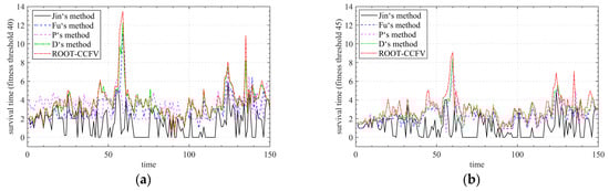

Figure 10.
The survival time of different algorithms under different fitness thresholds. (a) Fitness threshold = 40. (b) Fitness threshold = 45. (c) Fitness threshold = 50.
Table 3.
The average survival time of robust solutions under different algorithms.
From Figure 10 and Table 2, it can be seen that the robustness of the solution obtained by ROOT-CCFV is better than other existing ROOT methods proposed in references [29,30,33] when dealing with mMPB under different fitness thresholds. Taking the fitness threshold of 40 as an example, the average survival time of ROOT-CCFV under the current fitness threshold was 145.1%, 23.8%, 11.9% and 3.6% higher than that of Jin’s ROOT, Fu’s ROOT, P’s ROOT and D’s ROOT, respectively.
6.2.3. Analysis of RES Uncertainty under ROOT-CCFV Based on Scene Method
This section took the WT in the IA as an example to illustrate. Figure 11 shows the process of the scene analysis method based on LHS and BR, where Figure 11a is the generated wind speed in multiple scenarios based on LHS; based on BR, we reduced the large-scale scene and calculated the probability of each scene after reduction, as shown in Figure 11b; the output power of the WT in typical scenarios by (16) is shown in Figure 11c; and Figure 11d fits the typical wind power output power curve obtained by the scenario method.
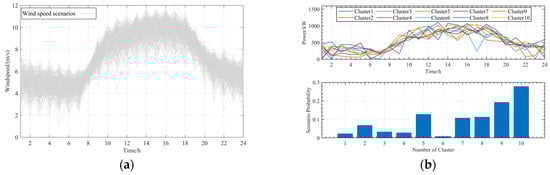

Figure 11.
Process of scene analysis method. (a) Scene generation based on LHS. (b) Scene reduction based on BR. (c) Calculated typical outpower power. (d) Curving fitting.
Based on the fitting curve of the RES in each region, the ROOT-CCFV was used to solve the optimal robust solution of the RES power output in each region. In order to verify the robustness of ROOT-CCFV, the algorithm was compared with stochastic optimization (SO) and fuzzy optimization (FO). The confidence interval of FO was set to 0.95. The robust solutions of RES output power under different algorithms are shown in Figure 12 and Figure 13.

Figure 12.
Robust solutions of the WT under different algorithms in the IA and OA.

Figure 13.
Robust solutions of PV under different algorithms in each region. (a) Robust solutions of PV in the RA and CA. (b) Robust solutions of PV in the IA and OA.
It can be seen from Figure 12 and Figure 13 that due to the robustness requirements for the stable operation of a RIES, the uncertainty prediction curves of the RES are slightly smaller than the actual RES output curve. Compared with the other two comparison algorithms, the prediction curve of ROOT-CCFV based on the scene method was closest to the actual output curve. Compared with SO, the curve of ROOT-CCFV was smoother. This is because under the ROOT-CCFV strategy, when the RES changes dynamically, the algorithm can obtain a more robust solution through and . Compared with FO, ROOT-CCFV can make the RIES obtain better economy under the premise of ensuring the robustness of optimal scheduling.
6.2.4. Analysis of SESS Capacity Configuration Considering EV Charging Demand
In order to study the influence of different EV charging models and RES uncertain calculation methods on SESS capacity configuration, the following four modes were set up.
Mode 1: The charging load of an EV was considered as a whole and it was charged only at RI; meanwhile, the SO was used to calculate the output power of the RES.
Mode 2: The charging loads of an EV were based on the trip chain proposed in this paper; meanwhile, the SO was used to calculate the output power of the RES.
Mode 3: The charging load of EV was considered as a whole and charged only at RI; meanwhile, the ROOT-CCFV was used to calculate the power output of an RES.
Mode 4: The charging loads of an EV were based on the trip chain proposed in this paper; meanwhile, the ROOT-CCFV was used to calculate the output power of the RES.
It was stipulated that the electric energy charged into an SESS is positive, indicating that each region charges the electric energy into SESS, the release of electric energy is negative, and indicating that each region is retrieving electric energy from SESS. The capacity configuration result of the SESS and the charging expenditure of the EV under different modes is shown in Table 4.
Table 4.
Capacity configuration of SESS and charging expenditure of EV under different modes.
Comparing the results of mode 1 and mode 2, and mode 3 and mode 4, respectively, it can be seen that under the same RES algorithm, the traditional EV charging model has a greater demand for SESS capacity and charging expenditure than the EV charging model based on the trip chain. This is because under the traditional EV charging, RI bears huge load pressure. In order to reduce the operating cost of the entire RIES, it is necessary to maintain sufficient SESS capacity to provide a power supply for RI, and a large number of EV charging loads are concentrated in RI, resulting in higher charging expenditure. Similarly, under the same RES algorithm, it can be seen that the charging expenditure of the EV charging model based on the trip chain was 3.6% and 3.1% lower than that of the traditional EV charging model, respectively. Therefore, the EV charging model proposed in this paper has better energy economy.
Comparing the results of mode 1 and mode 3, and mode 2 and mode 4, respectively, it can be seen that under the same EV charging model, the SESS capacity configuration under ROOT-CCFV was higher than that under SO. This is because under the premise of ensuring robustness, ROOT-CCFV can obtain a value closer to the actual RES output power through its strategy than SO. In order to reduce the operating expenditure, the RIES chooses to store the surplus RES in the SESS and retrieve it from the SESS to the load during the peak load period, so as to achieve the purpose of reducing the interaction cost with EPG during peak period. Therefore, more SESS capacity configuration is required in the case of ROOT-CCFV.
Upon further study of the influence of different scales of the EV charging load on SESS capacity configuration and the RIES operating cost, based on the EV trip chain charging demand model in this paper, the total electric load of the four regions without the EV was 229,220 kW on a typical scheduling day. Assuming that the scale of the EV charging load was equal to 15%/20%/25%/30%/35% of the total electric load, the results of the SESS capacity configuration and RIES operating cost are shown in Table 5.
Table 5.
The result of capacity configuration and operation cost under different EV load scales.
From Table 5, as the scale of the EV load continues to increase, the optimal configuration capacity of the SESS continues to decrease, and the operating cost of the RIES continues to increase. For the SESS, this is because when the EV load is large, each region needs to provide more power to the EV, and there is no more surplus RES stored in SESS, resulting in a reduction in the required capacity of SESS. For RIES, this is because each region needs to produce more electric power to meet the demand for the EV load.
6.2.5. Analysis of Optimal Scheduling Results of the RIES Considering the EV Charging Demand
Based on the four modes set out in Section 6.2.4, the influence of different EV charging models and the RES uncertainty calculation methods on RIES operating costs were studied. The details of RIES operation costs under different modes are shown in Table 6.
Table 6.
The details of RIES operating costs under different modes.
It can be seen from Table 6 that in the mode of the same use of ROOT-CCFV, the operating cost of the RIES under the EV charging demand based on the trip chain was 11.7% lower than that under the traditional EV charging demand model. In the same mode of using the EV charging demand based on the trip chain, the operating cost of the RIES under ROOT-CCFV was 6.9% lower than that of the RIES under SO. In summary, compared with the traditional EV charging demand modeling method, the EV charging demand model based on the trip chain can help the RIES obtain a capacity configuration result that is more in line with the actual energy demand, thereby reducing the operating cost of the RIES. Similarly, compared with SO, ROOT-CCFV can obtain more robust RES output power, reduce the interaction cost between the RIES and EPG, and thus reduce the operating cost of the RIES. Taking mode 4 as an example, the optimal scheduling results of each region in the RIES were analyzed and are described as follows.
The RIES electrical load optimization scheduling results are shown in Figure 14. It can be seen from Figure 14a that since the RA and CA only contain PV, the RA and CA purchase the required electrical energy from the EPG when PV has less output power or no output power. At the same time, when the EPG price is high, the RA and CA will also start the GT for power generation. From Figure 14b, it can be seen that because the IA and OA contain abundant RESs, excess power can be sold to EPG or stored in the SESS when the RES meets its own load demand. The IA and OA start the GT power generation to make up for the electric load gap only when the RES output power is not enough to meet their own load in the morning and evening.

Figure 14.
Electric load optimization scheduling results of the RIES. (a) Electric optimal scheduling of the RA and CA. (b) Electric optimal scheduling of the IA and OA.
The RIES electrical load optimization scheduling results are shown in Figure 15. From Figure 15, we can see that the GB is the main equipment to provide heat power for each region. It can be seen from Figure 15a that when the PV equipment starts to work during the 10:00–17:00 period, the RA and CA choose PV to provide electricity for the EB to provide the required heat energy in order to better reduce operating costs. From Figure 15b, it can be seen that for the IA and OA, their RES was mainly sold to the EPG for revenue, so their heat load was mainly provided by the GB.

Figure 15.
Heat load optimization scheduling results of the RIES. (a) Heat optimal scheduling of the RA and CA. (b) Heat optimal scheduling of the IA and OA.
The RIES cold load optimization scheduling results are shown in Figure 15. From Figure 16, we can see that the EC was the main equipment to provide heat power for each region. It can be seen from Figure 16a and previous analysis that the GT needs to provide power for the RA and CA when PV energy stops. At this time, the high-temperature waste heat generated by the GT was transmitted through the WHB, part of which was transmitted to the HE and converted into heat energy to meet the heat load demand, and part of which was transmitted to the AC and converted into cold energy to meet the cold load demand. For the IA and OA, from Figure 16b we can see that because they contain very rich RES, they mainly met their own demand for cooling load through the EC.

Figure 16.
Cold load optimization scheduling results of the RIES. (a) Cold optimal scheduling of the RA and CA. (b) Cold optimal scheduling of the IA and OA.
6.2.6. Analysis of IDR
The IDR optimization results are shown in Figure 17, Figure 18 and Figure 19. The RL according to the EPG price, in the period of a high electricity price, cut part of the load. The TL transferred the load in the high-energy-price period to the low-energy-price period, and reduced the operating costs while causing the load curve to tend to be smooth. When the electricity price per unit energy supply was higher than the price of cold/heat energy price, SL converted part of the cold/heat energy into electric load. The IDR model established in this paper makes the load curve smoother and realizes peak load shifting. In order to verify the effect of the IDR in RIES optimal scheduling, the following mode were set.

Figure 17.
Electric load IDR optimization results of the RIES. (a) Electric load IDR results of the RA and CA. (b) Electric load IDR results of the IA and OA.

Figure 18.
Heat load IDR optimization results of the RIES. (a) Heat load IDR results of the RA and CA. (b) Heat load IDR results of the IA and OA.

Figure 19.
Cold load IDR optimization results of the RIES. (a) Cold load IDR results of the RA and CA. (b) Cold load IDR results of the IA and OA.
Mode 5: based on mode 4 without considering the IDR.
Mode 6: based on mode 4 considering the IDR.
The details of RIES operating costs before and after considering the IDR are shown in Table 7. From Table 7, it can be seen that when the RIES considers the IDR model proposed in this paper, its optimal operating cost decreases from CNY 104,548.92 without considering the IDR model to CNY 99,502.61; the optimal operating cost decreases by 4.8%. In summary, the IDR model proposed in this paper can effectively reduce the operating cost of the RIES.
Table 7.
The details of RIES operating costs before and after the IDR.
7. Conclusions
Aiming at the optimal scheduling problem of an RIES with EVs, this paper first established a charging demand load mode of EV based on the trip chain theory; meanwhile, it established a multi-energy IDR model. Aiming at the uncertainty problem of an RES, firstly, the above problem was transformed into a class of dynamic robust optimization problems with time-varying parameters, and then a ROOT-CCFV algorithm based on a scenario method was proposed to solve this kind of problem. By establishing an RIES model containing four regions and conducting case studies, the following conclusions can be drawn:
- The ROOT-CCFV algorithm can better solve the dynamic optimization problem with time-varying parameters and obtain a more robust solution. Compared with the existing algorithms, in the mMPB test environment, the average survival time of the robust solution obtained by the ROOT-CCFV algorithm was increased by 46.1% on average. The proposed ROOT-CCFV algorithm provides a solution for solving dynamic optimization problems in the future.
- The reasonable modeling of an EV charging demand model can effectively reduce the capacity configuration cost of an SESS and the optimal operation cost of an RIES in this region. And the larger the EV load in the region, the less the SESS capacity required in the region. Under the same RES uncertainty solving algorithm, compared with the traditional EV charging model, the EV charging model based on the trip chain proposed in this paper can reduce the cost of its own charging expenditure by 3.5%, and at the same time reduce the operating cost of an RIES by 11.7%.
- The alternative IDR model proposed in this paper can realize the coupling of electric heating and cold energy, and effectively reduce the operation cost of an RIES. When the IDR model proposed in this paper is considered in RIES optimal scheduling, the operating cost can be reduced by 4.8%.
Author Contributions
Conceptualization, B.Z. and E.L.; methodology, B.Z. and E.L.; validation, E.L.; investigation, B.Z.; data curation, B.Z. and E.L.; writing—original draft preparation, B.Z.; writing—review and editing, B.Z. and E.L.; supervision, E.L.; funding acquisition, B.Z. and E.L. All authors have read and agreed to the published version of the manuscript.
Funding
This research was funded by National Nature Science Foundation of China, grant number 62063019. This research was funded by Natural Science Foundation of Gansu Province, grant number 22JR5RA241 and 2023CXZX-465.
Data Availability Statement
The data that support the findings of this study are available from the corresponding author upon reasonable request.
Conflicts of Interest
The authors declare no conflicts of interest.
Appendix A
Table A1.
Capacity parameters of equipment in each CCHP/(kWh).
Table A1.
Capacity parameters of equipment in each CCHP/(kWh).
| Equipment | RA | CA | IA | OA |
|---|---|---|---|---|
| PV | 2000 | 4000 | 8000 | 2000 |
| WT | / | / | 6000 | 3000 |
| ES | / | 1000 | 2000 | / |
| GT | 2000 | 5000 | 8000 | 3000 |
| WHB | 5000 | 5000 | 8000 | 5000 |
| GB | 5000 | 5000 | 8000 | 5000 |
| EH | 5000 | 5000 | 8000 | 5000 |
| EC | 5000 | 5000 | 8000 | 5000 |
| AC | 5000 | 5000 | 8000 | 5000 |
| HE | 4000 | 4000 | 4000 | 4000 |
Table A2.
Efficiency parameters of equipment in each CCHP.
Table A2.
Efficiency parameters of equipment in each CCHP.
| Equipment | RA | CA | IA | OA |
|---|---|---|---|---|
| Efficiency of GT | 0.35 | 0.35 | 0.35 | 0.35 |
| Heat-to-electric ratio of GT | 2.3 | 2.3 | 2.3 | 2.3 |
| Efficiency of WHB | 0.73 | 0.73 | 0.73 | 0.73 |
| Efficiency of GB | 0.85 | 0.85 | 0.85 | 0.85 |
| Efficiency of EH | 0.98 | 0.98 | 0.98 | 0.98 |
| Efficiency of EC | 4 | 4 | 4 | 4 |
| Efficiency of AC | 1.2 | 1.2 | 1.2 | 1.2 |
| Efficiency of HE | 0.9 | 0.9 | 0.9 | 0.9 |
| Maximum charging of ES | / | 200 kW | 400 kW | / |
| Maximum discharging of ES | / | 200 kW | 400 kW | / |
| Charging efficiency of ES | / | 0.95 | 0.95 | / |
| Discharging efficiency of ES | / | 0.95 | 0.95 | / |
| Self-discharging efficiency of ES | / | 0.04 | 0.04 | / |
| Initial energy storage of ES | / | 200 kWh | 400 kWh | / |
| Maximum energy storage of ES | / | 900 kWh | 1800 kWh | / |
| Minimum energy storage of ES | / | 200 kWh | 400 kWh | / |
Table A3.
Equipment parameters of an SESS.
Table A3.
Equipment parameters of an SESS.
| Parameter | Value | Parameter | Value |
|---|---|---|---|
| Charging efficiency | 0.95 | Initial state of SOC | 0.50 |
| Discharging efficiency | 0.95 | Maximum state of SOC | 0.90 |
| Self-discharging efficiency | 0.04 | Minimum state of SCO | 0.20 |
| Maximum charge/discharge power to each region | 1000 kW |
Table A4.
TOU electricity price of EPG (CNY/kWh).
Table A4.
TOU electricity price of EPG (CNY/kWh).
| RA | CA/IA/OA | ||||||
|---|---|---|---|---|---|---|---|
| Price Types | Time Interval | Purchase Price | Sale Price | Price Types | Time Interval | Purchase Price | Sale Price |
| Peak time | 07:00–09:00 18:00–24:00 | 0.759 | 0.415 | Peak time | 07:00–09:00 17:00–23:00 | 0.8650 | 0.415 |
| Usual time | 00:00–02:00 04:00–07:00 09:00–11:00 17:00–18:00 | 0.510 | 0.415 | Usual time | 23:00–00:00 00:00–07:00 | 0.5843 | 0.415 |
| Valley time | 02:00–04:00 11:00–17:00 | 0.261 | 0.415 | Valley time | 09:00–17:00 | 0.3036 | 0.415 |
Table A5.
TOU electricity price of an SESS (CNY/kWh).
Table A5.
TOU electricity price of an SESS (CNY/kWh).
| Price Types | Time Interval | Purchase Price | Sale Price |
|---|---|---|---|
| Peak time | 08:00–09:00, 19:00–24:00 | 0.725 | 0.435 |
| Usual time | 00:00–02:00, 05:00–07:00 10:00–11:00, 18:00–18:00 | 0.475 | 0.435 |
| Valley time | 03:00–04:00, 12:00–17:00 | 0.271 | 0.435 |
References
- European Commission. Horizon 2020 Work Programme 2018–2020: 10. Secure, Clean and Efficient Energy; Official Publications of the European Communities: Luxembourg, 2018. [Google Scholar]
- Zhou, S.; Han, Y.; Mahmoud, K.; Darwish, M.M.; Lehtonen, M.; Yang, P.; Zalhaf, A.S. A novel unified planning model for distributed generation and electric vehicle charging station considering multi-uncertainties and battery degradation. Appl. Energy 2023, 348, 121566. [Google Scholar] [CrossRef]
- Zhang, N.; Sun, Q.; Yang, L.; Li, Y. Event-Triggered Distributed Hybrid Control Scheme for the Integrated Energy System. IEEE Trans. Ind. Inform. 2021, 18, 835–846. [Google Scholar] [CrossRef]
- Liu, L.; Yao, X.; Qi, X.; Han, Y. Low-carbon economy configuration strategy of electro-thermal hybrid shared energy storage in multiple multi-energy microgrids considering power to gas and carbon capture system. J. Clean. Prod. 2023, 428, 139366. [Google Scholar] [CrossRef]
- Li, Y.; Han, M.; Yang, Z.; Li, G. Coordinating Flexible demand response and renewable uncertainties for scheduling of community integrated energy systems with an electric vehicle charging station: A bi-level approach. IEEE Trans. Sustain. Energy 2021, 12, 2321–2331. [Google Scholar] [CrossRef]
- Gan, L.; Chen, X.; Yu, K.; Zheng, J.; Du, W. A probabilistic evaluation method of household EVs dispatching potential considering users’ multiple travel needs. IEEE Trans. Ind. Appl. 2020, 56, 5858–5867. [Google Scholar] [CrossRef]
- Lan, T.; Jermsittiparsert, K.; Alrashood, S.T.; Rezaei, M.; Al-Ghussain, L.; Mohamed, M.A. An Advanced Machine Learning Based Energy Management of Renewable Microgrids Considering Hybrid Electric Vehicles’ Charging Demand. Energies 2021, 14, 569. [Google Scholar] [CrossRef]
- Taibi, E.; del Valle, C.F.; Howells, M. Strategies for solar and wind integration by leveraging flexibility from electric vehicles: The Barbados case study. Energy 2018, 164, 65–78. [Google Scholar] [CrossRef]
- Mwasilu, F.; Justo, J.J.; Kim, E.-K.; Do, T.D.; Jung, J.-W. Electric vehicles and smart grid interaction: A review on vehicle to grid and renewable energy sources integration. Renew. Sustain. Energy Rev. 2014, 34, 501–516. [Google Scholar] [CrossRef]
- Rassaei, F.; Soh, W.S.; Chua, K.C. Demand response for residential electric vehicles with random usage patterns in smart grids. IEEE Trans. Sustain. Energy 2015, 6, 1367–1376. [Google Scholar] [CrossRef]
- Tan, J.; Wang, L. Real-Time charging navigation of electric vehicles to fast charging stations: A hierarchical game approach. IEEE Trans. Smart Grid 2015, 8, 846–856. [Google Scholar] [CrossRef]
- Li, G.; Wu, D.; Hu, J.; Li, Y.; Hossain, M.S.; Ghoneim, A. HELOS: Heterogeneous load scheduling for electric vehicle-integrated microgrids. IEEE Trans. Veh. Technol. 2016, 66, 5785–5796. [Google Scholar] [CrossRef]
- Yu, M.; Hong, S.H. A real-time demand-response algorithm for smart grids: A stackelberg game approach. IEEE Trans. Smart Grid 2015, 7, 879–888. [Google Scholar] [CrossRef]
- Wang, D.; Guan, X.; Wu, J.; Li, P.; Zan, P.; Xu, H. Integrated energy exchange scheduling for multimicrogrid system with electric vehicles. IEEE Trans. Smart Grid 2015, 7, 1762–1774. [Google Scholar] [CrossRef]
- Husein, M.; Chung, I.-Y. Day-Ahead Solar Irradiance Forecasting for Microgrids Using a Long Short-Term Memory Recurrent Neural Network: A Deep Learning Approach. Energies 2019, 12, 1856. [Google Scholar] [CrossRef]
- Huang, Y.; Wang, L.; Guo, W.; Kang, Q.; Wu, Q. Chance constrained optimization in a home energy management system. IEEE Trans. Smart Grid 2016, 9, 252–260. [Google Scholar] [CrossRef]
- Baker, K.; Bernstein, A. Joint chance constraints in AC optimal power flow: Improving bounds through learning. IEEE Trans. Smart Grid 2019, 10, 6376–6385. [Google Scholar] [CrossRef]
- Zhang, Y.; Ai, Q.; Xiao, F.; Hao, R.; Lu, T. Typical wind power scenario generation for multiple wind farms using conditional improved Wasserstein generative adversarial network. Int. J. Electr. Power Energy Syst. 2020, 114, 105388. [Google Scholar] [CrossRef]
- Li, Y.; Wang, B.; Yang, Z.; Li, J.; Chen, C. Hierarchical stochastic scheduling of multi-community integrated energy systems in uncertain environments via Stackelberg game. Appl. Energy 2021, 308, 118392. [Google Scholar] [CrossRef]
- Li, Y.; Han, M.; Shahidehpour, M.; Li, J.; Long, C. Data-driven distributionally robust scheduling of community integrated energy systems with uncertain renewable generations considering integrated demand response. Appl. Energy 2023, 335, 120749. [Google Scholar] [CrossRef]
- Yang, J.; Su, C. Robust optimization of microgrid based on renewable distributed power generation and load demand uncertainty. Energy 2021, 223, 120043. [Google Scholar] [CrossRef]
- Huang, S.; Lu, H.; Chen, M.; Zhao, W. Integrated energy system scheduling considering the correlation of uncertainties. Energy 2023, 283, 129011. [Google Scholar] [CrossRef]
- Kalathil, D.; Wu, C.; Poolla, K.; Varaiya, P. The sharing economy for the electricity storage. IEEE Trans. Smart Grid 2017, 10, 556–567. [Google Scholar] [CrossRef]
- Dai, R.; Esmaeilbeigi, R.; Charkhgard, H. The utilization of shared energy storage in energy systems: A comprehensive review. IEEE Trans. Smart Grid 2021, 12, 3163–3174. [Google Scholar] [CrossRef]
- Kang, C.; Liu, J.; Zhang, N. A new form of energy storage in future power system: Cloud energy storage. Autom. Electr. Power Syst. 2017, 41, 2–8. [Google Scholar]
- Walker, A.; Kwon, S. Analysis on impact of shared energy storage in residential community: Individual versus shared energy storage. Appl. Energy 2020, 282, 116172. [Google Scholar] [CrossRef]
- Liu, N.; Tan, L.; Sun, H.; Zhou, Z.; Guo, B. Bilevel Heat–Electricity Energy Sharing for Integrated Energy Systems with Energy Hubs and Prosumers. IEEE Trans. Ind. Inform. 2021, 18, 3754–3765. [Google Scholar] [CrossRef]
- Jabir, H.J.; Teh, J.; Ishak, D.; Abunima, H. Impacts of Demand-Side Management on Electrical Power Systems: A Review. Energies 2018, 11, 1050. [Google Scholar] [CrossRef]
- Tang, D.; Wang, P. Probabilistic modeling of nodal charging demand based on spatial-temporal dynamics of moving electric vehicles. IEEE Trans. Smart Grid 2015, 7, 627–636. [Google Scholar] [CrossRef]
- Yu, X.; Jin, Y.; Tang, K.; Yao, X. Robust optimization over time—A new perspective on dynamic optimization problems. In Proceedings of the 2010 IEEE Congress on Evolutionary Computation, Barcelona, Spain, 18–23 July 2010; pp. 3998–4003. [Google Scholar]
- Jin, Y.; Tang, K.; Yu, X.; Sendhoff, B.; Yao, X. A framework for finding robust optimal solutions over time. Memetic Comput. 2013, 5, 3–18. [Google Scholar] [CrossRef]
- Fu, H.; Sendhoff, B.; Tang, K.; Yao, X. Finding Robust Solutions to Dynamic Optimization Problems. In Proceedings of the 16th European Conference on Applications of Evolutionary Computation, Vienna, Austria, 3–5 April 2013; pp. 616–625. [Google Scholar]
- Cao, M.; Shao, C.; Hu, B.; Xie, K.; Li, W.; Peng, L.; Zhang, W. Reliability Assessment of Integrated Energy Systems Considering Emergency Dispatch Based on Dynamic Optimal Energy Flow. IEEE Trans. Sustain. Energy 2021, 13, 290–301. [Google Scholar] [CrossRef]
- Lee, T.-K.; Bareket, Z.; Gordon, T.; Filipi, Z.S. Stochastic modeling for studies of real-world PHEV usage: Driving schedule and daily temporal distributions. IEEE Trans. Veh. Technol. 2012, 61, 1493–1502. [Google Scholar] [CrossRef]
- Novoa-Hernandez, P.; Pelta, D.A.; Corona, C.C. Approximation Models in Robust Optimization Over Time—An Experimental Study. In Proceedings of the 2018 IEEE Congress on Evolutionary Computation (CEC), Rio de Janeiro, Brazil, 8–13 July 2018; pp. 1–6. [Google Scholar] [CrossRef]
- Yazdani, D.; Nguyen, T.T.; Branke, J. Robust Optimization over Time by Learning Problem Space Characteristics. IEEE Trans. Evol. Comput. 2018, 23, 143–155. [Google Scholar] [CrossRef]
Disclaimer/Publisher’s Note: The statements, opinions and data contained in all publications are solely those of the individual author(s) and contributor(s) and not of MDPI and/or the editor(s). MDPI and/or the editor(s) disclaim responsibility for any injury to people or property resulting from any ideas, methods, instructions or products referred to in the content. |
© 2024 by the authors. Licensee MDPI, Basel, Switzerland. This article is an open access article distributed under the terms and conditions of the Creative Commons Attribution (CC BY) license (https://creativecommons.org/licenses/by/4.0/).