Evaluating Outdoor Performance of PV Modules Using an Innovative Explicit One-Diode Model

Abstract

Due to its simplicity, the one-diode model is commonly used for modeling the operation of photovoltaic (PV) modules at standard test conditions (STC). However, its inherent implicit nature often presents challenges in modeling PV energy production. In this paper, the innovative explicit one-diode model developed by us over time is adapted for estimating PV power production under real weather conditions. Simple yet accurate equations for calculating the energy output of a PV generator equipped with a maximum power point tracking (MPPT) system are proposed. The model’s performance is assessed under various normal and harsh operating conditions against measured data collected from the experimental setup located at the Solar Platform at West University of Timisoara, Romania. As an application of the new equation for maximum power, this paper presents a case study where the energy loss in the absence of an MPPT system is evaluated based on atmospheric and sky conditions.

1. Introduction

In recent years, significant increases in energy costs, particularly for natural gas, have impacted Europe and various other countries. Consequently, the transition towards adopting cleaner energy sources, notably solar power, is gaining momentum. In 2023, the International Energy Agency recommended installing approximately 60 GWp of solar power to offset the reduction in the gas market. As a result, nearly 17 million additional European households were powered by solar energy in 2023 due to a 40% growth in solar installations compared to 2022. Europe experienced a substantial increase in solar capacity, with 55.9 GWp of new installations in 2023 compared to 40 GWp in the previous year [1]. Moreover, 2023 marked a new era for solar energy in Central and Eastern Europe, as countries like the Czech Republic, Bulgaria, and Romania reached the threshold of at least 1 GWp of installed solar capacity a year. With the anticipated growth of solar capacity, the performance of PV modules becomes paramount in optimizing energy production [1].

The amount of incoming solar radiation and the cell temperature are the two principal factors that affect the performance of a PV module. To accurately estimate the power output of a PV module under various real weather conditions, it is necessary to have a thorough understanding of its current–voltage (I–V) characteristic. This characteristic graphically represents the relationship between the PV module’s current and voltage output [2], serving as a tool in assessing its operational efficiency. Manufacturers deliver a PV module with a datasheet, commonly containing information about the module’s electrical behavior with a focus on its I–V characteristic. A datasheet features three notable parameters of the I–V characteristic: the short-circuit current, open circuit voltage, and the maximum power point (MPP), all measured at standard test conditions (STC). STC implies a normal incoming solar radiation of 1000 W/m² under the AM1.5G spectrum [3] and a cell temperature of 25 °C. However, this limited information often falls short for intricate modeling, and there is a need for additional analysis to gain a more comprehensive understanding of the PV module’s performance.

In describing the operation of a PV module, most mathematical models are rooted in Shockley’s theory of the illuminated p–n junction [4]. Among these models, the one-diode model stands out due to its apparent simplicity. Based on the one-diode model equivalent circuit from Figure 1, the most widely used equation for the I–V characteristic of a solar cell is:

$$I=I_L-I_S\left[\exp \left(\frac{q\left(V+I{R}_S\right)}{m{k}_{B}T}\right)-1\right]-\frac{V+I{R}_S}{R_P}$$

(1)

where $q$ is the electron charge, $k_B$ is the Boltzmann constant, and T is the cell temperature. The photocurrent $I_L$, diode saturation current $I_S$, diode ideality factor $m$, serial resistance $R_S$, and shunt resistance $R_P$ form a set of five parameters (specific for a cell), which give the model its name, the five-parameter model.

Numerous studies focusing on the one-diode model have been developed in recent years. Parameter extraction under both STC and in real weather conditions [5], as well as PV performance assessment [6], has been the main area of interest.

The application of the one-diode model Shockley equation (Equation (1)) is often vulnerable to the inherent implicit nature of the equation. Parameter extraction demands iterative methods and excessive calculus. From a fundamental perspective, the explicit writing of the equation must be understood as a research goal in itself. Since this study is based on our proposal for an explicit equation (presented in Section 3), the current state of research in the field is briefly summarized next.

Over the years, numerous research efforts have been concentrated on formulating an explicit Shockley equation for one-diode equivalent circuits [7,8,9]. The choice of rewriting Shockley’s equation using a Lambert W function [10] is very popular. Lambert W is a special function which can be a tool in analytically modeling the performance of solar cells or panels. However, this function requires a complex solving process. The mathematical challenges in the function evaluation may not align with the interest of the PV industrial sector. The resulting explicit equations might still be perceived as excessively complex to be considered a “direct” equation [11]. Despite the various attempts to formulate an explicit equation, success has been limited. Generally, the explicit models are based on expressions that are not easy to manage. In other cases, some models are suitable only for PV cells, their performance being reduced when they are applied in the case of PV panels. Some attempts to explicitly write the one-diode model equation are summarized below.

A simplified form of the explicit equation of the one-diode model expressed by the Lambert W function is presented in [7]. The complex explicit equation is reduced to a simplified form through variable substitution. The simplified equation was integrated with an intelligent optimization algorithm to assess and estimate the parameters of the one-diode model. Ref. [12] presents an emulator for the static and dynamic characteristics of a PV panel. It uses an explicit PV model, which approximates the implicit equation by using the Taylor series. The authors emphasize that the methodology eliminates the necessity of numerous iterative computations. Ref. [13] introduces an explicit equation starting from the one-diode model decomposition. The voltage across the diode in the equivalent circuit acts as an independent variable and makes the curve computation explicit. The authors claim that the method outperforms the Newton–Raphson and the Lambert W algorithms. Implicit and explicit models for different PV modules technologies are compared in [14].

Figure 2 illustrates the impact of solar irradiance level and cell temperature variations on the current–voltage characteristics of a PV module. The output current of the module exhibits no remarkable changes despite temperature shifts. Moreover, variations in solar radiation levels exhibit a notable influence on the PV module’s current output in contrast to its voltage. It is noteworthy that these fluctuations lead to variations in the overall output power of a PV module.

The maximum power point (MPP) in PV systems represents the peak output power that the system reaches. As Figure 2 shows, its position on the I–V characteristic dynamically shifts in response to the variations in solar radiation and temperature. This directly impacts the expected output power, as PV systems are designed to generate a predetermined power level. Ensuring optimal power generation from the PV generator requires tracking of the MPP. Consequently, maximum power point tracking (MPPT) algorithms are vital in continuously monitoring and adjusting for fluctuations in the MPP. The fundamental concept of MPPT implies optimizing the power output of a PV module by dynamically adjusting its operating point on the I–V characteristic, aiming to align it with the voltage that maximizes efficiency. MPPT entails continuous monitoring of the PV module’s output, juxtaposing it with the battery voltage, and subsequently determining the optimal power output that the module can deliver. Various MPPT techniques can be categorized based on their tracking methods into four main groups: classical, intelligent, optimization, and hybrid methods. The efficiency of each tracking technique varies depending on its ability to monitor peak power under dynamic environmental conditions [2]. A PV emulator for the static and dynamic characteristics of a PV module based on I–V explicit modeling and its straightforward application to MPPT are studied in [12]. Ref. [15] presents an algorithm for the MPP based on solving a single-variable equation. Its unique solution leads to an explicit expression of the point by using a parametrization of the one-diode model I–V curve. While numerous MPPT methods for PV systems are extensively discussed in the literature, a review of them, as undertaken in [16], is beyond the scope of this study.

A comprehensive review of PV system modeling and parameter extraction is presented in [17]. The authors also present a one-diode model that describes the I–V and P–V characteristics of a PV module in different operating conditions. The model can be used as a potential tool for PV system design and installation in fluctuating weather conditions, and also for MPPT or fault investigation. Ref. [18] has developed a technique for PV power prediction under varying irradiance and temperature levels employing one- and two-diode models. The experimental validation of the models is carried out at specific ground-measured solar radiation and temperature to check the accuracy of the estimated PV power output.

This study aims to assess the performance of PV modules in outdoor conditions through the application of our explicit one-diode model equation. The form of the equation is innovative, comprising the ideal Shockley equation along with an additive term [19]. The proposed equation removes the implicit nature of the one-diode model equation, making it easier to obtain the model parameters at STC. In this study, the equation is completed and adapted for estimating PV power under real weather conditions. A novel straightforward yet accurate equation for calculating the output power of a PV generator equipped with an MPPT system is proposed. The use of an explicit model for the emulation of the I–V characteristic contributes to the efficiency of the MPP calculation and, consequently, of the MPP tracking technique.

The paper is organized as follows. The database used in this study is described in Section 2. Section 3 presents our innovative explicit one-diode model designed to assess the outdoor performance of a PV module. As a case study, a comprehensive discussion on applying the proposed model to the MPP calculation is presented in Section 4. The main conclusions are gathered in Section 5.

2. Database

In this study, data collected from the experimental setup located at the Solar Platform at West University of Timisoara were processed [20]. The FORPV setup (Figure 3) was designed to assess models used for estimating and forecasting PV power. It consists of a 540 Wp PV system comprising four Cleversolar SPR-135 PV modules facing to the south, tilted at a 30-degree angle, and connected in a series–parallel configuration. These modules directly supply power to a resistive load. To measure the in-plane solar irradiance, a high-quality Kipp & Zonen SMP-10 pyranometer (class A according to ISO9060:2018) is employed. Additionally, meteorological data are recorded using a Delta-T Devices WS-GP2 weather station. Continuous monitoring of these instruments is conducted around the clock, with data recorded at regular intervals of 4 s. Furthermore, an EKO Instruments ASI-16 all-sky imager is used for monitoring the state of the sky at 1-min sampling.

A database consisting of records for 46 days, from March and April 2023, was created. The days were selected to cover periods significantly different from each other in terms of solar radiative regime. As spring days were the focus, most of the days exhibit instability in the state of the sky. Clouds may introduce uncertainty in the PV power estimation due to the diffuse nature of the incident light. In cloudy conditions, the in-plane direct solar irradiance is suppressed (and thus its confidence on the incidence angle), and total solar irradiance essentially depends on cloud transparency. For further analyses, the database was divided into classes of relative sunshine, $\sigma$ (Figure 4). This parameter describes (indirectly) the state of the sky during the daytime, being defined as:

$$\sigma =\frac{s}{S}$$

(2)

where $S$ is the length of a given time interval and $s$ is the bright sunshine duration during that interval. Usually, $S$ is the period between sunrise and sunset (in hours), while $s$ denotes the number of daily bright sunshine hours. Shorter $S$ intervals are used, as in the case of this study where data from 8 a.m. till 4 p.m. are used. Naturally, a low $\sigma$ is an indicator of a high amount of cloud cover.

3. Development of the Explicit One-Diode Model

The one-diode model parameters are commonly determined through an algorithm, irrespective of its specific methodology, that deals with highly non-linear equations derived from Equation (1). However, there is still no widely accepted standardized method for extracting the one-diode model parameters. The obtained set of parameters is crucial for accurately replicating the I–V characteristic at STC, and thus for estimating the output power of a PV module. A good set of parameters enables reliable projections of the performance in estimating the output power in real weather scenarios.

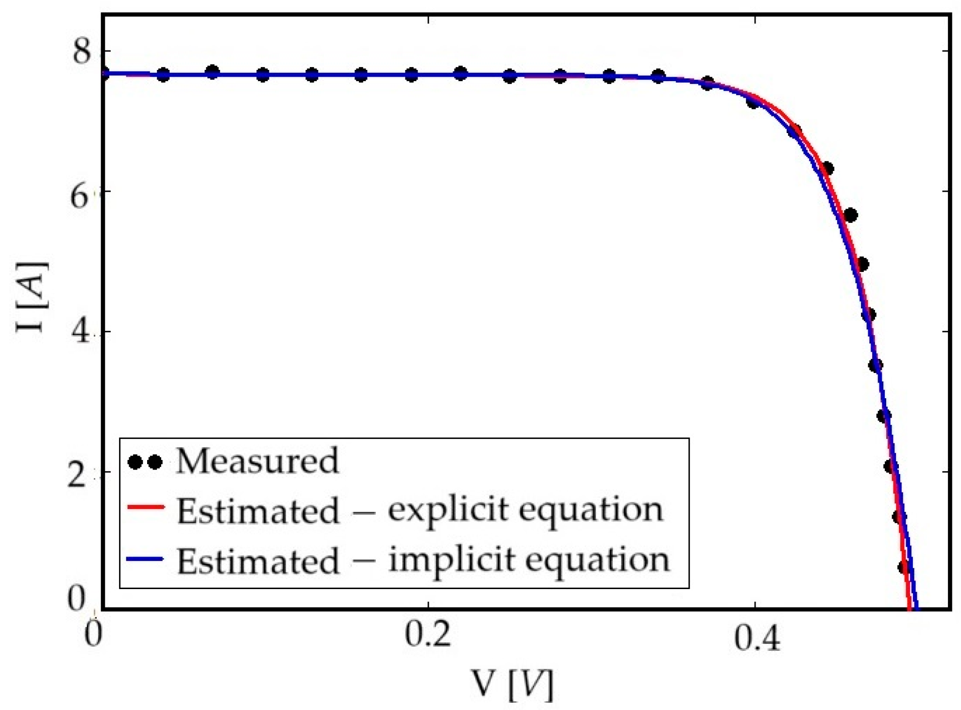
3.1. Explicit One-Diode Model Equation at STC

What sets this study apart from previous research in this field is its pioneering utilization of an explicit one-diode model equation:

$$I=I_L-I_S\left[\exp \left(\frac{qV}{m{k}_{B}T}\right)-1\right]-\frac{V}{R_P}+g\left(V\right)$$

(3)

Equation (3) represents the generic explicit equation of our one-diode model. The additive term g(V) represents the innovative element of the model. g(V) encapsulates an explicit expression for compensating for the assumption $R_S=0$ in Equation (1). Equation (3) simplifies the process of parameter extraction from measured data at STC. This approach contributes to avoiding the potential issue of an algorithm being trapped in a local minimum, thereby enhancing the efficiency and reliability of parameter extraction.

The form of g(V) is obtained from Equations (3) and (1). This involves an approximation, namely, expressing the exponential term $\exp \left(\frac{qI{R}_S}{m{k}_{B}T}\right)$ through the Taylor series and retaining only the first two terms. This is the only approximation in deriving $g\left(V\right)$ and is assessed further in this section. After further simplifying the calculus, the final equation for g(V) is obtained:

$$g\left(V\right)=\frac{\left[-I_S\frac{q{R}_S}{m{k}_{B}T}\exp \left(\frac{qV}{m{k}_{B}T}\right)-\frac{R_S}{R_P}\right]\left[I_L-I_S\left[\exp \left(\frac{qV}{m{k}_{B}T}\right)-1\right]-\frac{V}{R_P}\right]}{1+\frac{R_S}{R_P}+I_S\frac{q{R}_S}{m{k}_{B}T}\exp \left(\frac{qV}{m{k}_{B}T}\right)}$$

(4)

A detailed calculation of the term g(V) is provided as Supplementary Materials.

Replacing Equation (4) in Equation (3) results in an explicit equation for the current–voltage equation. After some algebraic calculations, a simple, elegant, mathematical expression is obtained:

$$I=\frac{I_L-I_S\left[\exp \left(\frac{qV}{m{k}_{B}T}\right)-1\right]-\frac{V}{R_P}}{1+\frac{R_S}{R_P}+I_S\frac{q{R}_S}{m{k}_{B}T}\exp \left(\frac{qV}{m{k}_{B}T}\right)}$$

(5)

Equation (5) represents a true explicit equation of the one-diode model of a PV converter.

In this study, Equation (5) was used to replicate the measured I–V characteristic of the Cleversolar SPR-135 PV modules installed at the Solar Platform at West University of Timisoara at STC. For this, a successive discretization algorithm (SDA) [21] was applied. Among many solutions, one set of parameters was retained, exhibiting a coefficient of determination, $R^2$, of 0.997 (

Table 1. One-diode model parameters obtained with the SDA. The algorithm was applied to Equations (1) and (5) in the same computational framework.

Equation	Parameters					${\mathit{R}}^2$
	${\mathit{I}}_{\mathit{L}}\left[\mathbf{A}\right]$	${\mathit{I}}_{\mathit{S}}[\mathbf{A}]$	$\mathit{m}$	${\mathit{R}}_{\mathit{S}}\left[\mathbf{\Omega }\right]$	${\mathit{R}}_{\mathit{P}}\left[\mathbf{\Omega }\right]$
Implicit Equation (1)	7.67	10−7	1.070	0.0022	23.2	0.990
Explicit Equation (5)	7.67	10−7	1.061	0.001	13	0.997

). $R^2$ is a measure of how well a model fits a set of data. Table 1 shows that significant differences between parameters appear when estimating the serial R_S and shunt R_P resistances.

Figure 5 illustrates the I–V characteristics at STC for the Cleversolar SPR-135 PV module, evaluated with the implicit (Equation (1)) and explicit (Equation (5)) equations. The equation parameters were estimated with the SDA in the same computational framework. The overlap between the measured and estimated I–V characteristic is remarkably close.

However, a better approximation of the measurements is observed for the I(V) curve generated by the explicit equation (Equation (5)). Although, to the naked eye, the difference between the curves seems small, the improvement of the characteristic is significant on the portion of steep variation. The result is confirmed by the increase of the determination coefficient R² in Table 1. This enhances the feasibility of the explicit one-diode model equation, Equation (5), in accurately replicating the measured I–V characteristic at STC and of its further use under real weather conditions. In addition, we stress again that the basic merit in employing the explicit equation is that it establishes a clear correlation between variables and leads to faster implementation. From the running time perspective, applying SDM to the explicit equation (Equation (5)) reduces the running time by 10% compared to the implicit equation (Equation (1)). For example, the running time decreases from 6.4 s to 5.6 s in the case of calculating the parameters at STC for the curves in Figure 5. The applications were run on an ordinary laptop.

3.2. One-Diode Model under Real Weather Conditions

As already mentioned, the two key factors that affect the efficiency and performance of the PV module are incoming solar radiation and temperature. Consequently, the parameters obtained at STC must be adapted to these real weather conditions to accurately estimate the output power of the PV module. Additionally, the degree of cleanliness of the module’s surface must be considered [22]. Our procedure from [19] offers notable advantages, characterized by its simplicity and accuracy. The procedure implies the parameters computed at STC and the following assumptions:

1.

The effective solar irradiance G_eff is determined taking into account the degree of cleanliness of the PV module:

$$G_{eff}={\tau }_{C}G$$

(6)

where ${\tau }_C$ is the cleanliness coefficient (

Table 2. The cleanliness coefficient as defined in [9].

Cleanliness Degree	Perfect	Proper	Medium	Low
${\tau }_C$	1.00	0.98	0.96	0.92

).

2.

The operating temperature of the solar cell is calculated as:

$$T=T_a+\frac{NOCT-20 °\mathrm{C}}{800}{G}_{eff}$$

(7)

where T_a denotes the ambient temperature and NOCT is the nominal operating cell temperature.

3.

The photocurrent is linearly linked with the incident solar irradiance and can be obtained by considering the thermal coefficient of the short-circuit current α_I

$$I_L\left(G,T\right)=I_{L,STC}\left[1+{\alpha }_I\left(T-T_{STC}\right)\right]\frac{G_{eff}}{G_{STC}}$$

(8)

4.

The saturation current is determined as:

$$I_S\left(G,T\right)=I_L\left(G,T\right)\exp \left[-\frac{q{V}_{OC,STC}\left[1+{\alpha }_V\left(T-T_{STC}\right)\right]}{m{k}_{B}T}\right]$$

(9)

where ${\alpha }_V$ is the thermal coefficient.

5.

The diode ideality factor and the series resistance and shunt resistance remain the same as at STC:

$$m=m_{STC},R_S=R_{S,STC},R_P=R_{P,STC}$$

(10)

For any set of parameters, this method facilitates the computation of the I–V characteristic of the PV module in real operating conditions defined by air temperature, solar irradiance, and degree of cleanness of the PV modules. By employing this procedure, we can obtain a better understanding of how the PV module performs under varying environmental conditions.

Figure 6 illustrates a comparison between the estimated and measured output power delivered by the PV system during the test days. Notably, the estimated power replicates the measured power with reasonable accuracy. There can be seen to be a very good overlap between the values, although slight differences can be observed for higher values. The normalized mean bias error nMBE calculated for the dataset is only 4.8%. nMBE is defined as $nMBE=100\cdot {\displaystyle \sum _{i=1}^n\left(e_i-m_i\right)}/{\displaystyle \sum _{i=1}^n{m}_i}$, where e and m denote the estimated and measured quantities, respectively. This test validates the model for further applications. From the running time perspective, using the explicit equation (Equation (5)) reduces the running time by two-thirds compared to the implicit equation (Equation (1)). For example, the running time decreases from 4.3 s to 1.3 s in the case of estimating the output power delivered by the PV system during the 46 test days.

3.3. Explicit One-Diode Model at MPP

In order to calculate the output power of a PV system, the explicit equation (Equation (5)) adapted to all weather conditions can be directly used:

$$P\left(V\right)=I\left(V\right)\cdot V$$

(11)

At the optimal operating point MPP, further denoted as $M(V_M,I_M)$, the output power reaches its maximum, $P_M=V_M{I}_M$. MPPT ensures that the PV system operates at the point of maximum power. By setting the derivative $dP/dV$ to zero, we impose the operation of the PV system at full power.

$$\frac{dP(V)}{dV}=\frac{\partial I(V)}{\partial V}V+I(V)=0$$

(12)

By differentiating $I(V)$ with respect to $V$, we obtain a rather complicated equation:

$$\frac{\partial I(V)}{\partial V}=\frac{-\frac{q{I}_S}{m{k}_{B}T}\exp \left(\frac{qV}{m{k}_{B}T}\right)-\frac{1}{R_P}}{1+\frac{R_S}{R_P}+\frac{q{I}_S{R}_S}{m{k}_{B}T}\exp \left(\frac{qV}{m{k}_{B}T}\right)}-\frac{q^2{I}_S{R}_S\exp \left(\frac{qV}{m{k}_{B}T}\right)\left[I_L-I_S\left(\exp \left(\frac{qV}{m{k}_{B}T}\right)-1\right)-\frac{V}{R_P}\right]}{{\left(m{k}_{B}T\right)}^2{\left(1+\frac{R_S}{R_P}+\frac{q{I}_S{R}_S}{m{k}_{B}T}\exp \left(\frac{qV}{m{k}_{B}T}\right)\right)}^2}$$

(13)

By replacing Equation (13) in Equation (12), we are able to solve the equation and to obtain the optimal values $(V_M,I_M)$. Equation (12) becomes an explicit equation, which represents a significant advantage from the computational point of view.

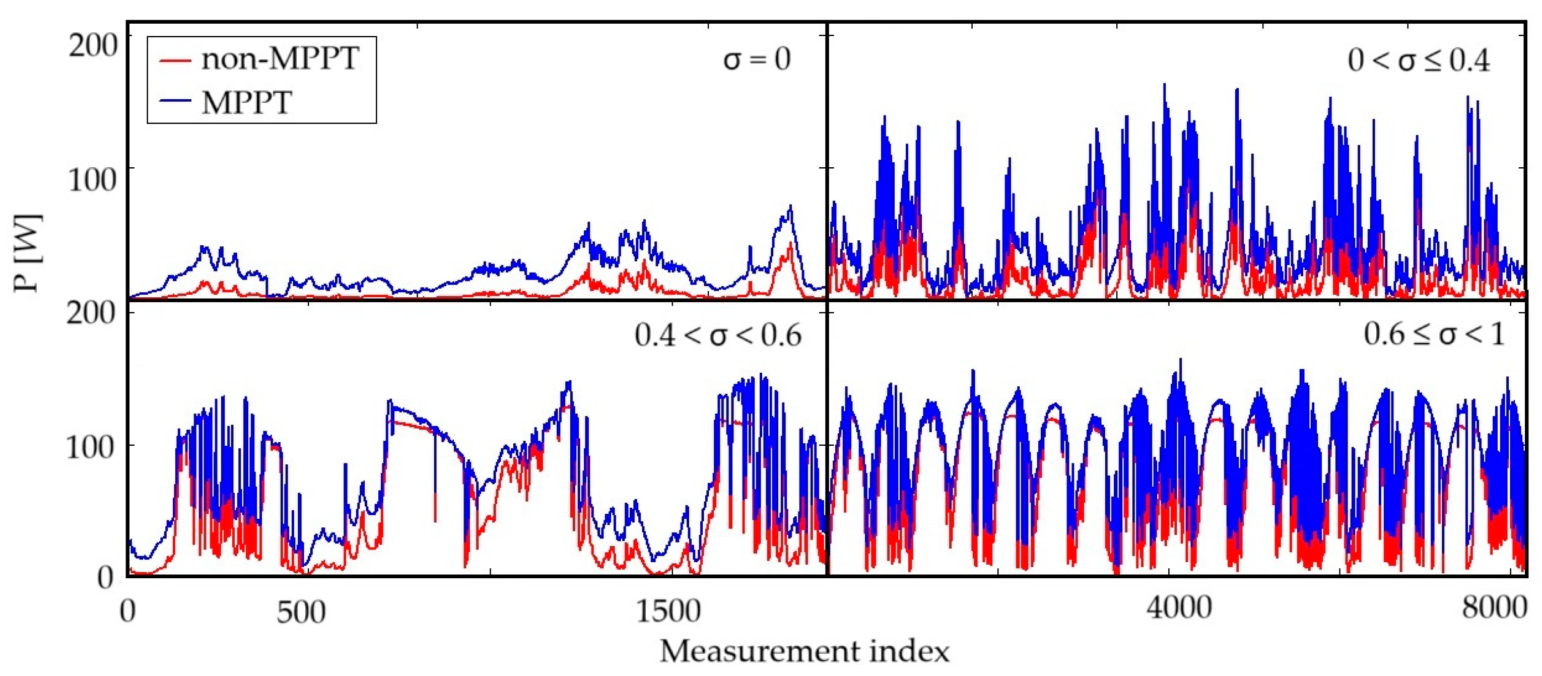
4. MPPT Performance: A Case Study

In this section we present the results of the comparison of the power delivered by the PV system in the test days, assuming the presence and the absence of MPPT. On the Solar Platform, the PV system is used for testing PV power models; thus, the PV modules are connected directly to a resistive load, without an MPPT system. The presence of MPPT was simulated with our explicit model. The dataset was divided into four distinct classes based on relative sunshine levels. More specifically, $\sigma =0$ (5 days), meaning no sunshine during the day; $0<\sigma \le 0.4$ (20 days) and $0.4<\sigma <0.6$ (4 days), representing varying degrees of cloud cover during the day; and $0.6\le \sigma <1$ (17 days), meaning a lower cloud coverage with longer periods of sunshine.

Figure 7 graphically compares the measured power (in the absence of MPPT) with the estimated power in the presence of MPPT. The results highlight the effectiveness of MPPT, especially during overcast conditions. As can be seen in

Table 3. Relative error values for each class of relative sunshine.

Relative Sunshine $\mathit{\sigma }$	Relative Error [%]
$\sigma =0$	76.9
$0<\sigma \le 0.4$	45.1
$0.4<\sigma <0.6$	23.9
$0.6\le \sigma <1$	13.4

, in overcast conditions the implementation of MPPT technologies demonstrates a potential to extract an additional 77% of the available power on a pure resistive load. Moreover, considering the characteristics of the dataset (spring days, with colder temperatures), it is evident that MPPT substantially reduces losses, particularly in scenarios featuring both lower temperatures and high cloud coverage. In instances of low cloud coverage throughout the day, the losses covered by MPPT are only 13%. There are two significant moments during a day when the output power obtained with both a fixed resistive load and MPPT overlap, one preceding and one following midday, as depicted in Figure 8. Besides those two moments, the load line never intersects the I–V characteristic in the MPP. Figure 8 presents a randomly selected day from the database for illustrative purposes, the observed behavior being consistent across all days.

5. Conclusions

The inherent implicit nature of the one-diode model equation presents challenges in modeling PV power production. Removing the implicit mathematical relationship has long been a research topic. This study introduces an innovative explicit one-diode model designed for estimating PV power production under real weather conditions. New accurate equations for calculating the PV power at the MPP are provided. The model demonstrates good accuracy in estimating the output power of a PV system operating in various normal and harsh weather conditions. The model equations are given in detail, facilitating easy and fast implementation in customized PV applications.

The results presented in the paper can have a potential impact both theoretically and practically. From the scientific point of view, writing an explicit equation represents an important result per se, as it enables a general way to suppress the interdependence in the common one-diode PV module equation. Following the theoretical development proposed in this paper, explicit equations can be developed for the I–V characteristic of any solar cell that can be modeled at different degrees of approximation in terms of the implicit Shockley equation. The explicit equation for the one-diode equivalent circuit of a PV module with an additional term represents an innovation. The coupling with simple equations of adaptation to real environmental conditions brings applicability in current practice. The derivation of an explicit equation for determining the MPP is another significant gain. From the practical point of view, the results indicate comparable or better accuracy than that of the implicit equation. At the same estimation accuracy, the net advantage of the explicit method is from the computational point of view. The implementation of the explicit equations is obviously easier, and the tests show a significant reduction of the computation time: roughly 10% in the case of running SDM and two-thirds in the case of output power estimation for a PV system operating in real environmental conditions.

References

1. IEA. World Energy Outlook 2023; IEA: Paris, France, 2023; Available online: https://www.iea.org/reports/world-energy-outlook-2023 (accessed on 1 April 2024).
2. Paulescu, M.; Paulescu, E.; Gravila, P.; Badescu, V. Weather Modeling and Forecasting of PV Systems Operation; Springer: London, UK, 2013. [Google Scholar]
3. Reference Air Mass 1.5 Spectra. 2024. Available online: https://www.nrel.gov/grid/solar-resource/spectra-am1.5.html (accessed on 1 April 2024).
4. Nelson, J. The Physics of Solar Cells; Imperial College Press: London, UK, 2013. [Google Scholar]
5. Yang, B.; Wang, J.; Zhang, X.; Yu, T.; Yao, W.; Shu, H.; Zeng, F.; Sun, L. Comprehensive overview of metaheuristic algorithm applications on PV cell parameter identification. Energy Convers. Manag. 2020, 208, 112595. [Google Scholar] [CrossRef]
6. Wang, M.; Peng, J.; Luo, Y.; Shen, Z.; Yang, H. Comparison of different simplistic prediction models for forecasting PV power output: Assessment with experimental measurements. Energy 2022, 224, 120162. [Google Scholar] [CrossRef]
7. Li, J.; Qin, C.; Yang, C.; Ai, B.; Zhou, Y. Extraction of single diode model parameters of solar cells and PV modules by combining an intelligent optimization algorithm with simplified equation based on Lambert W function. Energies 2023, 16, 5425. [Google Scholar] [CrossRef]
8. Saloux, E.; Teyssedou, A.; Sorin, M. Explicit model of photovoltaic panels to determine voltages and current at the maximum power point. Sol. Energy 2011, 85, 713–722. [Google Scholar] [CrossRef]
9. Lun, S.; Du, C.; Yang, G.; Wang, S.; Guo, T.; Sang, J.; Li, J. An explicit approximate I-V characteristic model of a solar cell based on pade approximants. Sol. Energy 2013, 92, 147–159. [Google Scholar] [CrossRef]
10. Corless, R.M.; Gonnet, G.H.; Hare, D.E.G.; Jeffrey, D.J.; Knuth, D.E. On the Lambert W function. Adv. Comput. Math. 1996, 5, 329–359. [Google Scholar] [CrossRef]
11. Roibas-Millan, E.; Cubero-Estalrrich, J.L.; Gonzalez-Estrada, A.; Jado-Puente, R.; Sanabria-Pinzon, M.; Alfonso-Corcuera, D.; Alvarez, J.M.; Cubas, J.; Pindado, S. Lambert W-function simplified expressions for photovoltaic current-voltage modelling. In Proceedings of the 2020 IEEE International Conference on Environment and Electrical Engineering and 2020 IEEE Industrial and Commercial Power Systems Europe (EEEIC/I&CPS Europe), Madrid, Spain, 9–12 June 2020; pp. 1–6. [Google Scholar]
12. Alombah, N.H.; Harrison, A.; Kamel, S.; Fotsin, H.B.; Aurangzeb, M. Development of an efficient and rapid computational solar photovoltaic emulator utilizing an explicit PV model. Sol. Energy 2024, 271, 112426. [Google Scholar] [CrossRef]
13. Mathew, L.E.; Panchal, A.K. An exact and explicit PV panel curve computation assisted by two 2-port networks. Sol. Energy 2022, 240, 280–289. [Google Scholar] [CrossRef]
14. Boutana, N.; Mellit, A.; Lughi, V.; Pavan, M. Assessment of implicit and explicit models for different photovoltaic modules technologies. Energy 2017, 122, 128–143. [Google Scholar] [CrossRef]
15. Toledo, F.J.; Galiano, V.; Herranz, V.; Blanes, J.M.; Batzelis, E. A comparison of methods for the calculation of all the key points of the PV single-diode model including a new algorithm for the maximum power point. Optim. Eng. 2023, 1–35. [Google Scholar] [CrossRef]
16. Katche, M.L.; Makokha, A.B.; Zachary, S.O.; Adaramola, M.S. A Comprehensive Review of Maximum Power Point Tracking (MPPT) Techniques Used in Solar PV Systems. Energies 2023, 16, 2206. [Google Scholar] [CrossRef]
17. Humada, A.M.; Darweesh, S.Y.; Mohammed, K.G.; Kamil, M.; Mohammed, S.F.; Kasim, N.K.; Tahseen, T.A.; Awad, O.I.; Mekhilef, S. Modeling of PV system and parameter extraction based on experimental data: Review and investigation. Sol. Energy 2020, 199, 742–760. [Google Scholar] [CrossRef]
18. Kumar, M.; Malik, P.; Chandel, R.; Chandel, S.S. Development of a novel solar PV module model for reliable power prediction under real outdoor conditions. Renew. Energy 2023, 217, 119224. [Google Scholar] [CrossRef]
19. Sabadus, A.; Paulescu, M. A New Explicit Five-Parameter Solar Cell Model. In Proceedings of the 8th World Conference on Photovoltaic Energy Conversion (WCPEC-8 2022), Milan, Italy, 26–30 September 2023; pp. 454–456. [Google Scholar] [CrossRef]
20. Solar Platform of the West University of Timisoara, Romania. Available online: http://solar.physics.uvt.ro/srms/ (accessed on 1 May 2024).
21. Cotfas, D.T.; Deaconu, A.M.; Cotfas, P.A. Application of successive discretization algorithm for determining photovoltaic cells parameters. Energy Convers. Manag. 2019, 196, 545–556. [Google Scholar] [CrossRef]
22. Paulescu, M.; Badescu, V.; Dughir, C. New performance and field-test to assess photovoltaic module performance. Energy 2014, 70, 49–57. [Google Scholar] [CrossRef]
Figure 1. One-diode equivalent circuit of a solar cell.
Energies 17 02547 g001
Figure 2. I–V and P–V characteristics of a solar module under varying (a,c) solar irradiance and (b,d) cell temperature.
Energies 17 02547 g002
Figure 3. FORPV experimental setup located at the Solar Platform at West University of Timisoara, Romania.
Energies 17 02547 g003
Figure 4. Relative sunshine, σ , for all the 46 test days. The shaded areas denote missing data: 7th of March (incomplete) and 22nd–29th of March (system stopped).
Energies 17 02547 g004
Figure 5. The I–V characteristic at STC for the Cleversolar SPR-135 PV module evaluated with the implicit (Equation (1)) and explicit (Equation (5)) equations, whose parameters were estimated in the same computational framework.
Energies 17 02547 g005
Figure 6. Measured vs estimated output power delivered by the PV system for 46 days in March and April 2023.
Energies 17 02547 g006
Figure 7. Measured power vs power obtained with MPPT.
Energies 17 02547 g007
Figure 8. Highlight of the overlap of MPPT with measured data.
Energies 17 02547 g008