Investigations of Energy Conversion and Surface Effect for Laser-Illuminated Gold Nanorod Platforms

Abstract

Achieving a quick temperature increase is a burning issue for biophysical applications, like germ inactivation and tumor ablation, and for energy performances, like solar collectors and steam generators. Based on the plasmon resonance phenomenon, noble metallic nanoparticles have emerged as promising weapons due to their very high biocompatibility, optical properties, and high surface-to-volume ratio, increasing energy conversion and allowing the maximum temperature to be reached faster. This work examines the energy conversion in sandwiched glassy platforms with gold nanorods. The platforms are kept vertically in the air and illuminated by a 0.5 W near-infrared laser (808 nm). To describe this aspect theoretically, the size and conversion efficiency of the electromagnetic properties are compromised between the proposed model and the stability of the nanorods. As a research approach, our model of cross-sections and polarizability for the surface effect is proposed, coupled with classical CFD numerical calculations. The results of the proposed model, validated by a thermal camera and spectroscopy measurements, indicate that as long as the energy conversion is visible with relatively low-power lasers (ΔT = 18.5 °C), the platforms do not offer fast heat dissipation. The results indicate that, despite the flow forcing by the air inflow, the entropy generation due to heat conduction is more than three orders higher than the dynamic entropy production. Flow forcing corresponds to the value of the velocity for classical convective motions. Therefore, the delivered heat flux must be distributed via convective transport or the associated high-conductive materials.

1. Introduction

Fossil fuels have dominated the world’s energy sources for ages due to their widespread availability. However, it has recently been discovered that their exploitation and widespread consumption are hastening the greenhouse effect. As a result, in recent years, the diligent search for new alternative energy sources and their diversification has become a burning issue [1,2]. However, the majority of renewable energy sources do not provide an instant and powerful temperature increase that can last for hours, or they drastically raise the usage costs. Unfortunately, many of the available techniques are based on supplying heat flux to a fluid–solid boundary, implying the slow temperature increase throughout the system.

People realized the importance of hand and room disinfection during the COVID-19 pandemic. Unlike powerful chemical compounds, overheating can reduce the number of germs and viruses in a specific volume to nearly zero. Similarly, tumors and cancers may be totally eradicated; however, there exists the same challenge: how can we avoid destroying healthy cells whilst maintaining the noninvasive ones [3,4,5].

Metallic nanoparticles are emerging as a new strategy due to their own radiative properties. Moreover, their ability to travel through microscale pipes and their high heat transfer coefficient provides a quicker temperature rise than in standard metal sheet heat transfer. Therefore, the future vision generally is to apply these nanomaterials to solar collectors, steam production, and germ inactivation. Although several papers have proposed solutions for nanofluidic flows in the context of mass and heat transfer [6,7,8,9], heat generation in nanoparticles is still in its infancy, and the nanoparticle shape optimization necessitates the numerical computation of sophisticated formulae and equations, extending the time of a single simulation.

This paper extends the theoretical model presented in the authors’ previous papers [4,10,11,12,13] with continuum lasers and highlights the aspects that increase the energy conversion. The presented approach aims to use the validated theories, like the Cattaneo–Vernotte equation, the Rayleigh–Drude approximation, and the electromagnetic energy conversion into heat from the localized-surface plasmon resonance phenomenon. This allows for the study of the electrical field regardless of the nanoparticle’s shape, although the model appears to produce dissatisfactory results in the blue and UV regions due to the Rayleigh limitation [14,15,16,17,18,19]. Section 2 details these topics particularly for the computational fluid dynamics (CFD) (Section 2.1) equations, energy conversion (Section 2.2), and electric field distribution (Section 2.3) with the influence of the gold nanorods deposited on the charged surface (Section 2.4) [20,21,22].

Furthermore, Section 3.1 illustrates the numerical proceedings and discretized geometry, which were tested on mesh and with time independence to ensure minimal numerical errors [23,24]. In Section 3.3, all the boundary conditions supporting the convection and radiation processes are presented, as well as the material properties that were used to solve all the necessary CFD equations [7,25,26,27].

The mesh and time independence tests are described in Section 4.1. Section 4.2 presents the validation results confirming the validity of the adopted methodology. The results of further analysis (Section 4.3) take into account the movement of the fluid during the heating and cooling process. The discussion of the results and a summary are presented in Section 4.4 and Section 5, respectively.

At this stage, it is worth emphasizing that despite the extraordinary importance of the experimental results carried out to obtain the temperature field from a thermal camera and spectroscopy measurements, they do not impart knowledge about the velocity fields and entropy generation in the area of the resulting system. Therefore, one of the goals of this work was the numerical analysis of the temperature field, velocity, and entropy generation in the area where the measurements were not made.

The main purpose of this study was to investigate how a quick temperature increase affects the heat and mass flow around gold nanorod platforms. Several investigations have already touched upon this topic [27,28,29,30], although they concern different nanomaterials under the forced convection process and not the natural one, which is stated to be dominant in this case. Moreover, in contrast to the well-known heat sources, laser beams encourage the use of Gaussian distribution in the space regime, which implies interesting and promising properties, that are worth studying.

2. Theoretical Models

2.1. CFD Governing Equations

The heat transfer of light-illuminated metallic nanoparticles is generally calculated using various methods, depending on the considered model and the working light source. The majority of them require the use of the hyperbolic energy equation, also known as the Cattaneo–Vernotte equation [14,15], which is given by

$$\mathsf{\Gamma }·\frac{{\partial }^2}{{\partial t}^2}\left(\rho ·e\right)+\frac{\partial }{\partial t}\left(\rho ·e\right)+\mathrm{d}\mathrm{i}\mathrm{v}\left(\rho ·e\overrightarrow{v}\right)=\mathrm{d}\mathrm{i}\mathrm{v}\left(k_{\mathrm{e}\mathrm{f}\mathrm{f}}·\mathrm{g}\mathrm{r}\mathrm{a}\mathrm{d}\left(T\right)+\left(\left(\stackrel{⃡}{\tau }-p\stackrel{⃡}{ℐ}\right)·\overrightarrow{v}\right)\right)+S_e^{\mathrm{f}}+S_e^{\mathrm{n}\mathrm{p}}$$

(1)

This equation requires the establishment of the relaxation time, $\mathsf{\Gamma }$, which defines the finite speed of heat propagation, and which is satisfied for crystalline solids by

$$\mathsf{\Gamma }=\frac{3·k_{\mathrm{e}\mathrm{f}\mathrm{f}}}{\rho ·{c_p}_{\mathrm{e}\mathrm{f}\mathrm{f}}}·{\left(\frac{1}{v_d}\right)}^2$$

(2)

For noble metals, however, this value equals circa ${10}^{-10} \mathrm{s}$, and, as may be realized, the Cattaneo–Vernotte equation can be easily reduced to the standard parabolic one if the CW- and millipulsed light sources are considered, as is performed in this paper.

Hence, the standard energy equation, associated with the continuity, momentum, turbulence, and dissipation equations, which are based on the standard $\mathbb{k}$-$\mathcal{E}$ computational fluid dynamics (CFD) model for flows and the Boussinesq approach, is represented in this work by the following equations [12]:

$$\frac{\partial }{\partial t}\left\{\begin{array}{c}\begin{array}{c}\rho \\ \rho \overrightarrow{v}\\ \rho e\end{array}\\ \rho \mathbb{k}\\ \rho \mathcal{E}\end{array}\right\}+\mathrm{d}\mathrm{i}\mathrm{v}\left\{\begin{array}{c}\begin{array}{c}\begin{array}{c}\rho \overrightarrow{v}\\ \rho \overrightarrow{v}⨂\overrightarrow{v}\\ \rho e\overrightarrow{v}\end{array}\\ \rho \mathbb{k}\overrightarrow{v}\end{array}\\ \rho \mathcal{E}\overrightarrow{v}\end{array}\right\}=\mathrm{d}\mathrm{i}\mathrm{v}\left\{\begin{array}{c}\begin{array}{c}\begin{array}{c}0\\ \stackrel{⃡}{\tau }-p\stackrel{⃡}{ℐ}\\ \left(\stackrel{⃡}{\tau }-p\stackrel{⃡}{ℐ}\right)·\overrightarrow{v}+k_{\mathrm{e}\mathrm{f}\mathrm{f}}·\mathrm{g}\mathrm{r}\mathrm{a}\mathrm{d}\left(T\right)\end{array}\\ \left(\mu +\frac{{\mu }_{\mathbb{t}}}{{\mathrm{P}\mathrm{r}}_{\mathbb{k}}}\right)·\mathbb{k}\end{array}\\ \left(\mu +\frac{{\mu }_{\mathbb{t}}}{{\mathrm{P}\mathrm{r}}_{\mathcal{E}}}\right)·\mathcal{E}\end{array}\right\}+\left\{\begin{array}{c}\begin{array}{c}\begin{array}{c}0\\ \left(\rho -{\rho }_o\right)·\overrightarrow{g}\\ S_e^{\mathrm{f}}+S_e^{\mathrm{n}\mathrm{p}}\end{array}\\ G_{\mathbb{k}}-\rho \mathcal{E}+G_{\mathsf{Б}}\end{array}\\ C_{1ϵ}·\frac{\mathcal{E}}{\mathbb{k}}·\left(G_{\mathbb{k}}+C_{3\mathcal{E}}·G_{\mathsf{Б}}\right)-C_{1ϵ}·\rho ·\frac{{\mathcal{E}}^2}{\mathbb{k}}\end{array}\right\}$$

(3)

where

$$\stackrel{⃡}{\tau }=\mathrm{g}\mathrm{r}\mathrm{a}\mathrm{d}\left(\overrightarrow{X^{†}}\right)-\frac{2}{3}\mu {ℐ}_{\stackrel{⃡}{d}}\stackrel{⃡}{ℐ}+2\mu \stackrel{⃡}{d}$$

(4)

$$G_{\mathbb{k}}=2{\mu }_{\mathbb{t}}·\stackrel{⃡}{d}·{\stackrel{⃡}{d}}^T$$

(5)

$$G_{\mathsf{Б}}=\mathsf{Б}·\frac{{\mu }_{\mathbb{t}}}{\mathrm{P}\mathrm{r}}·\overrightarrow{g}·\mathrm{g}\mathrm{r}\mathrm{a}\mathrm{d}\left(T\right)$$

(6)

$$\stackrel{⃡}{\mathbb{R}}=-\frac{2}{3}(\rho \mathbb{k}+{\mu }_{\mathbb{t}}{ℐ}_{\stackrel{⃡}{d}})\stackrel{⃡}{ℐ}+2{\mu }_{\mathbb{t}}\stackrel{⃡}{d}$$

(7)

Furthermore, the total entropy generation, $\mathbb{S}$, is investigated as the sum dynamic and static entropy:

$$\mathbb{S}={\mathbb{S}}_s+{\mathbb{S}}_d$$

(8)

Static entropy generation is defined in classical expression [28,29], as follows:

$${\mathbb{S}}_s=\frac{(k_{\mathrm{e}\mathrm{f}\mathrm{f}}+k_{\mathbb{t}})}{T}·{\mathrm{g}\mathrm{r}\mathrm{a}\mathrm{d}\left(T\right)}^2$$

(9)

Using the Boussinesq and turbulent methods with Formula (7), it is possible to determine dynamic entropy generation [30,31], as follows:

$${\mathbb{S}}_d =\left(\frac{\mu }{T}\right)·\left(-\frac{2}{3}\mu {ℐ}_{\stackrel{⃡}{d}}\stackrel{⃡}{ℐ}+2\stackrel{⃡}{d}\right)+\left(\frac{1}{T}\right)·\left(-\frac{2}{3}(\rho \mathbb{k}+{\mu }_{\mathbb{t}}{ℐ}_{\stackrel{⃡}{d}})\stackrel{⃡}{ℐ}+2{\mu }_{\mathbb{t}}\stackrel{⃡}{d}\right)$$

(10)

The total entropy generation parameter determines the irreversibility of each process and may also indicate, alongside the Richardson number, which type of convection, forced or natural, dominates in each simulation stage.

2.2. Energy Conversion Rate

The most relevant aspect in this work is to estimate this part of incident light energy that is directly responsible for energy conversion to heat. In the standard energy equation, this is described by a user-defined function, which is referred in this work as $S_e^{\mathrm{f}}$ and $S_e^{\mathrm{n}\mathrm{p}}$, respectively, for fluids and nanoparticles. Some assumptions, however, should be considered in this case.

Firstly, if a laser beam falls onto the surface at a low incident angle, the problem is easily reduced to the semi-infinite methods and Lambert–Beer–Bourger law, for which the heat generation formulae for thin films are satisfied by [4,7,10,13,16]

$$S_e^{\mathrm{f}}={A_{abs}}_M·I_{{abs}_M}={A_{abs}}_M·I_o\left(\overrightarrow{r}\right)·\left(1-R_M\right)·\left(1-\exp \left(-{A_{abs}}_M·\delta \right)\right)$$

(11)

where the absorption coefficient is represented by

$${A_{abs}}_M=\frac{4\pi ·\mathbb{i}\mathbb{m}\left(n_M\left(\lambda \right)\right)}{\lambda }$$

(12)

This approach is validated and commonly used, both for continuous media and porous structures (see Figure 1a). Hence, it has been assumed that nanoparticles can be treated as inclusions in a $\delta$-thick slab, and each of them contributes to the total energy conversion (Figure 1b) by the following formula:

$$\begin{gathered} S_e^{\mathrm{n}\mathrm{p}}=\sum _i^{{\mathbb{W}}_i}{w}_i·\sum _j^{{\mathbb{W}}_j}{w}_j·\sum _{\mathbb{L}}^{{\mathbb{W}}_{\mathbb{L}}}{w}_{\mathbb{L}}·\left({A_{abs}}_{i,j,\mathbb{L}}·{I_{abs}}_{i,j,\mathbb{L}}\right)= \\ \sum _i^{{\mathbb{W}}_i}{w}_i·\sum _j^{{\mathbb{W}}_j}{w}_j·\sum _{\mathbb{L}}^{{\mathbb{W}}_{\mathbb{L}}}{w}_{\mathbb{L}}·\left({A_{abs}}_{i,j,\mathbb{L}}·I_o\left(\overrightarrow{r}\right)·\left(1-R_{gl}\right)·\left(1-R_{i,j,\mathbb{L}}\right)·\left(1-\exp \left(-{A_{abs}}_{i,j,\mathbb{L}}·{\delta }_i\right)\right)\right) \end{gathered}$$

(13)

where $w_i$, $w_j$, and $w_{\mathbb{L}}$ are polydispersive (distribution) parameters, respectively, for size, length, and distance, and ${\delta }_i$ is the thickness at which the electric dipoles can occur, declared as the slab thickness. Here, it is assumed as the size of capped nanoparticles, written by the following:

$${\delta }_i={d_s}_i+2·d_g$$

(14)

Moreover, the optical coefficients, $A_{abs}$, are calculated differently, depending on the materials. Classical Maxwell equations imply that the incident light may convert the electromagnetic energy if the absorbed light is determined. For nanoparticles, this is described by the photothermal efficiency equation:

$${\eta }_{{PT}_{i,j,\mathbb{L}}}=\frac{I_{abs}}{I_{ext}}\cong \frac{{C_{abs}}_{i,j,\mathbb{L}}}{{C_{ext}}_{i,j,\mathbb{L}}}$$

(15)

and it refers only to nanoparticles. Hence, this is not the parameter that reflects the total efficiency but only facilitates absorbance spectroscopy measurements. The total energy conversion efficiency indicates the absorbed part over the incoming light, which is presented as follows:

$${\eta }_{{TOT}_{i,j,\mathbb{L}}}=\frac{I_{abs}\left(\overrightarrow{r}\right)}{I_o\left(\overrightarrow{r}\right)}\cong \left(1-R_{gl}\right)·\left(1-R_{i,j,\mathbb{L}}\right)·\left(1-\exp \left(-{A_{abs}}_{i,j,\mathbb{L}}·{\delta }_i\right)\right)$$

(16)

This is purposely emphasized to highlight what the standard laser beams imply, when assuming the normal distribution, according to the following formula:

$$I_o\left(\overrightarrow{r}\right)\to I_{oMax}·\exp \left(-2·{\left(\frac{\overrightarrow{r}}{{\mathcal{R}}_B}\right)}^2\right)$$

(17)

where ${\mathcal{R}}_B$ is the beam size.

2.3. Cross-Sections and Polarizability

For a perfect crystal structure, the energy conversion is governed by the diffuse transport of electrons in lattice. Generally, two-temperature models are used to calculate the heat exchange between electrons and crystal lattice. For nanoparticles, however, boundary effects are extremely crucial to be included. In this work, the plasmon resonance phenomenon suggests that electrons cannot be treated separately, but as collective vibrations over the whole nanoparticle. Since the vibrations are confined by a capping agent or a surface, they convert and release the accumulated energy as heat. In this work, this phenomenon is determined by optical cross-sections, which were primarily studied in papers by Mie and Lorentz [17,18], but their theories were too complex for nanostructures other than spheres. Hence, the Rayleigh–Drude approximation is considered to be validated as long as the following condition is satisfied:

$$\frac{\lambda }{2\mathsf{\pi }}>{\left(\stackrel{̿}{{d_s}^2·d_l}\right)}^{\frac{1}{3}}$$

(18)

Then, general assumptions of this theory refer particularly to nanoparticles illuminated by visible and infrared lasers. The representative optical cross-sections are described by [17,18]

$$\begin{gathered} {A_{abs}}_{i,j,\mathbb{L}}={\eta }_{{PT}_{i,j,\mathbb{L}}}{·\xi }_{i,j,\mathbb{L}}·{C_{ext}}_{i,j,\mathbb{L}}{=\xi }_{i,j,\mathbb{L}}·\left(\left({C_{ext}}_{i,j,\mathbb{L}}\right)-\left({C_{sca}}_{i,j,\mathbb{L}}\right)\right)= \\ {\xi }_{i,j,\mathbb{L}}·\left(\left(4\pi ·\left(\frac{2\pi }{\lambda }\right)·\mathbb{i}\mathbb{m}\left({\alpha }_{i,j,\mathbb{L}}\right)\right)-\left(\frac{8\pi }{3}·{\left(\frac{2\pi }{\lambda }\right)}^4·{\left|{{\alpha }_{\mathrm{e}\mathrm{f}\mathrm{f}}}_{i,j,\mathbb{L}}\right|}^2\right)\right) \end{gathered}$$

(19)

As can be seen, the cross-sections, ${C_{ext}}_{i,j,\mathbb{L}}$ and ${C_{sca}}_{i,j,\mathbb{L}}$, as an average electric field distribution, can be described easily by the effective parameter, ${{\mathsf{\alpha }}_{\mathrm{e}\mathrm{f}\mathrm{f}}}_{\mathrm{i},\mathrm{j},\mathbb{L}}$. For capped ellipsoids, this is assumed as (for Cartesian coordinates)

$${{\alpha }_{\mathrm{e}\mathrm{f}\mathrm{f}}}_{i,j,\mathbb{L}}=\frac{2}{3}·\left({\left({\alpha }_{i,j,\mathbb{L},y}\right)}_{-}+{\left({\alpha }_{i,j,\mathbb{L},z}\right)}_{-}\right)+\frac{1}{3}·\left({\left({\alpha }_{i,j,\mathbb{L},x,dl}\right)}_{+}\right)$$

(20)

and for the considered axis, $\widehat{i}$, it is

$${\alpha }_{i,j,\mathbb{L},\widehat{i}}=\frac{V_{{\mathrm{c}}_{i,j}}+V_{{\mathrm{g}}_{i,j}}}{4\pi }·\frac{\left({\epsilon }_{\mathrm{g}}-{\epsilon }_h\right)·\left({\epsilon }_{\mathrm{s}}+\left({\epsilon }_{\mathrm{c}}-{\epsilon }_{\mathrm{g}}\right)·\left({\mathsf{Л}}_{i,j,\mathbb{L},\widehat{i},\mathrm{c}}-{\delta }_i{·\mathsf{Л}}_{i,j,\mathbb{L},\widehat{i},\mathrm{g}}\right)\right)+\left(\frac{V_{{\mathrm{c}}_{i,j}}}{V_{{\mathrm{c}}_{i,j}}+V_{{\mathrm{g}}_{i,j}}}\right)·{\epsilon }_{\mathrm{g}}·\left({\epsilon }_{\mathrm{c}}-{\epsilon }_{\mathrm{g}}\right)}{\left({\epsilon }_h+\left({\epsilon }_{\mathrm{g}}-{\epsilon }_h\right){·\mathsf{Л}}_{i,j,\widehat{i},\mathrm{g}}\right)·\left({\epsilon }_{\mathrm{g}}+\left({\epsilon }_{\mathrm{c}}-{\epsilon }_{\mathrm{g}}\right)·\left({\mathsf{Л}}_{i,j,\mathbb{L},\widehat{i},\mathrm{c}}-{\delta }_i{·\mathsf{Л}}_{i,j,\mathbb{L},\widehat{i},\mathrm{g}}\right)\right)+\left(\frac{V_{{\mathrm{c}}_{i,j}}}{V_{{\mathrm{c}}_{i,j}}+V_{{\mathrm{g}}_{i,j}}}\right){·\mathsf{Л}}_{i,j,\mathbb{L},\widehat{i},\mathrm{g}}·{\epsilon }_{\mathrm{g}}·\left({\epsilon }_{\mathrm{c}}-{\epsilon }_{\mathrm{g}}\right)}$$

(21)

where $c$, $g$, and $h$ refer to core, agent, and host (working medium), respectively, and $+$ indicates the oriented direction amongst the Cartesian coordinates, $x$, $y$, and $z$.

For rods, however, the polarizability is modified by including the correction for flat dimensions (Figure 1). It was introduced primarily in Fuchs’ publication [19] that the elongation parameter (${\varphi }_{i,j}$) or depolarization factor (${\mathsf{Л}}_{i,j}$) may indicate that the opposite charges prefer to be accumulated at edges, generating dipoles. Hence, as long as these parameters tend to 1.0 in ellipsoids, wires, or disks, the situation changes significantly in rods. Then, the flat, long dimension contributes to configuring new dipoles. This is clearly visible in Figure 2, where each axis projection is illustrated. Subsequently, an update to the effective polarizability yields the following:

$$\begin{gathered} {{\alpha }_{\mathrm{e}\mathrm{f}\mathrm{f}}}_{i,j,\mathbb{L}}=\frac{2}{3}\left(\frac{2}{3}·\left({\left({\alpha }_{i,j,\mathbb{L},y}\right)}_{-}+{\left({\alpha }_{i,j,\mathbb{L},z}\right)}_{-}\right)+\frac{1}{3}·\left({\left({\alpha }_{i,j,\mathbb{L},x,dl}\right)}_{+}\right)\right)+ \\ \frac{1}{3}·\left(\frac{2}{3}·\left({\left({\alpha }_{i,j,\mathbb{L},y,ds}\right)}_{-}+{\left({\alpha }_{i,j,\mathbb{L},z,ds}\right)}_{-}\right)+\frac{1}{3}·\left({\left({\alpha }_{i,j,\mathbb{L},x}\right)}_{+}\right)\right) \end{gathered}$$

(22)

Although the effective parameter facilities including size, shape, distance, and surface effects, there is virtually zero examined reports studying the influence of these effects on the energy conversion. To calculate temperature distributions, however, the interaction between fluid and particles is primarily considered as an empirical boundary condition. For instance, the Smoluchowski approach investigates the heat transfer coefficient as the effective parameter for heat transfer [10,14,19,31]. The model, however, is well described for two boundaries, and nanostructures deposited on a loaded surface necessitate the use of a surface effect where at least three different materials must be considered.

2.4. Surface Effect

The possibility of implementing the effective polarizability offers a way to adjust different effects to achieve the most satisfactory approach. Formulae (19) and (20) have considered the case where a single nanoparticle is located in a soluble medium or deposited on an unloaded surface, such as glass. In this work, however, a 3 nm polyelectrolyte material (PEL) whose preparation and chemical processing enable creating ions, which tend to dissociate at the boundaries, is used. The creation of a negative charge contributes to modifications in the electric field through quasi-dipole-induced dipole interactions, as seen in the PEL-AuNR case. This affects the energy conversion as well as increasing the effective polarizability, ${{\alpha }_{\mathrm{e}\mathrm{f}\mathrm{f}}}_{i,j,\mathbb{L}}$, and the slab thickness, ${\delta }_i$. The sandwiched structure and the scheme of electric field distribution are revealed in Figure 3.

The topic, known as a surface effect, has been studied particularly in the literature for different geometries and parameters. The most common approximation is to assume the arithmetic mean of either permittivities [17] or polarizabilities [20] between the working fluid and base material, which provides only qualitative results. Other models assume the electric field-based results, which become complex for shapes other than spheres [20]. Here, the Royer–Yamaguchi approach [21] is claimed to provide satisfactory results due to the simplicity of combination surface and distance effect altogether. Although the model is dedicated to oblate structures, some corrections for rods based on Equations (20)–(22) require transformations that are necessary to be accomplished.

Having taken into account the nanoparticles’ orientation and the projection on the $x$-axis, the substrate calculations can be presented as follows:

$${\left({\alpha }_{i,j,\mathbb{L},x/z}\right)}_{-}=\frac{{\left({\alpha }_{i,j,x/z}\right)}_{sur}}{1+\left(\frac{{\left({\alpha }_{i,x/z}\right)}_{sur}}{\frac{4}{3}\pi ·{{d_s}_{c,i}}^2·{d_l}_{c,j}}\right)·{\beta }_{{\left|\right|}_{i,j,\mathbb{L}}}}$$

(23)

$${\left({\alpha }_{i,j,\mathbb{L},y}\right)}_{-}=\frac{{\left({\alpha }_{i,j,y}\right)}_{sur}}{1+\left(\frac{{\left({\alpha }_{i,j,y}\right)}_{sur}}{\frac{4}{3}\pi ·{{d_s}_{c,i}}^2·{d_l}_{c,j}}\right)·{\beta }_{{\perp }_{i,j,\mathbb{L}}}}$$

(24)

$${\left({\alpha }_{i,j,x}\right)}_{sur}=\left(\frac{{-\left(\frac{{d_s}_{c,i}}{2}\right)}^3·{\left(\frac{1-{{\varphi }_{i,j}}^2}{{{\varphi }_{i,j}}^2}\right)}^{\frac{1}{2}}}{3·{\mathbb{q}}_{11}\left(\mathbb{i}·{\left(\frac{1-{{\varphi }_{i,j}}^2}{{{\varphi }_{i,j}}^2}\right)}^{\frac{1}{2}}\right)}·\frac{{\epsilon }_c-{\epsilon }_h}{{\epsilon }_{\mathrm{c}}-{\mathbb{e}}_{11}\left(\mathbb{i}·{\left(\frac{1-{{\varphi }_{i,j}}^2}{{{\varphi }_{i,j}}^2}\right)}^{\frac{1}{2}}\right)}\right)$$

(25)

$${\left({\alpha }_{i,j,y}\right)}_{sur}=\left(\frac{{2·\left(\frac{{d_s}_{c,i}}{2}\right)}^3·\left(\frac{1}{{\varphi }_{i,j}}\right)}{3·{\mathbb{q}}_{10}\left(\mathbb{i}·{\left(\frac{1-{{\varphi }_{i,j}}^2}{{{\varphi }_{i,j}}^2}\right)}^{\frac{1}{2}}\right)}·\frac{{\epsilon }_c-{\epsilon }_h}{{\epsilon }_c-{\mathbb{e}}_{10}\left(\mathbb{i}·{\left(\frac{1-{{\varphi }_{i,j}}^2}{{{\varphi }_{i,j}}^2}\right)}^{\frac{1}{2}}\right)}\right)$$

(26)

$${\left({\alpha }_{i,j,z}\right)}_{sur}=\left(\frac{{2·\left(\frac{{d_s}_{c,i}}{2}\right)}^3·\left(\frac{1}{{\varphi }_{i,j}}\right)}{3·{\mathbb{q}}_{11}\left(\mathbb{i}·{\left(\frac{1-{{\varphi }_{i,j}}^2}{{{\varphi }_{i,j}}^2}\right)}^{\frac{1}{2}}\right)}·\frac{{\epsilon }_c-{\epsilon }_h}{{\epsilon }_c-{\mathbb{e}}_{11}\left(\mathbb{i}·{\left(\frac{1-{{\varphi }_{i,j}}^2}{{{\varphi }_{i,j}}^2}\right)}^{\frac{1}{2}}\right)}\right)$$

(27)

$${\mathbb{e}}_{\mathsf{\Lambda }\mathsf{{\rm M}}}=\frac{{\mathbb{p}}_{\mathsf{\Lambda }\mathsf{{\rm M}}}\left(\mathbb{i}·{\left(\frac{1-{{\varphi }_{i,j}}^2}{{{\varphi }_{i,j}}^2}\right)}^{\frac{1}{2}}\right)·{\left(\frac{d{\mathbb{q}}_{\mathsf{\Lambda }\mathsf{{\rm M}}}\left(\mathbb{i}·\psi \right)}{d\psi }\right)}_{\psi ={\left(\frac{1-{{\varphi }_{i,j}}^2}{{{\varphi }_{i,j}}^2}\right)}^{\frac{1}{2}}}}{{\mathbb{q}}_{\mathsf{\Lambda }\mathsf{{\rm M}}}\left(\mathbb{i}·{\left(\frac{1-{{\varphi }_{i,j}}^2}{{{\varphi }_{i,j}}^2}\right)}^{\frac{1}{2}}\right)·{\left(\frac{d{\mathbb{p}}_{\mathsf{\Lambda }\mathsf{{\rm M}}}\left(\mathbb{i}·\psi \right)}{d\psi }\right)}_{\psi ={\left(\frac{1-{{\varphi }_{i,j}}^2}{{{\varphi }_{i,j}}^2}\right)}^{\frac{1}{2}}}}$$

(28)

and distance effect, according to the paper by Royer [21]:

$${\beta }_{{\left|\right|}_{i,j,\mathbb{L}}}=\frac{\frac{4}{3}\pi ·{{d_s}_{c,i}}^2·{d_l}_{c,j}}{{\epsilon }_{sur}+{\epsilon }_h}·\left(\frac{-\left({\epsilon }_{sur}-{\epsilon }_h\right)}{{\left({d_s}_{c,i}+d_g\right)}^3}+\frac{2}{{\epsilon }_o·{\epsilon }_h}·\frac{\left(1-3·{\left(\frac{u_{\mathbb{L}}}{\sqrt{{u_{\mathbb{L}}}^2+{\left({d_s}_{c,i}+d_g\right)}^2}}\right)}^2\right)}{{u_{\mathbb{L}}}^3}\right)$$

(29)

$${\beta }_{{\perp }_{i,j,\mathbb{L}}}=\frac{\frac{4}{3}\pi ·{{d_s}_{c,i}}^2·{d_l}_{c,j}}{{\epsilon }_{sur}+{\epsilon }_h}·\left(\frac{-2·\left({\epsilon }_{sur}-{\epsilon }_h\right)}{{4\pi ·\epsilon }_o·{\epsilon }_w·{\left({d_s}_{c,i}+d_g\right)}^3}+\frac{2·{\epsilon }_{sur}}{{\epsilon }_o·{\epsilon }_h}·\left(\frac{1}{{u_{\mathbb{L}}}^3}\right)\right)$$

(30)

where the prolation parameter, ${\varphi }_{i,j}$, specifies the selected projection, as highlighted in Figure 2. From Formula (22),${\varphi }_{i,j,x}$, ${\varphi }_{i,j,y,z}$, ${\varphi }_{i,j,x, dl}$, ${\varphi }_{i,j,y,z, dl}$, ${\varphi }_{i,j,y,z, ds}$, and ${\varphi }_{i,j,x, ds}$ are determined as follows:

$${\varphi }_{i,j,x}=\sqrt{1-{\left(\frac{{d_s}_i}{{d_l}_j}\right)}^2}$$

(31)

$${\varphi }_{i,j,y,z}=\sqrt{1-{\left(\frac{0}{{d_l}_j}\right)}^2}=0$$

(32)

$${\varphi }_{i,j,x, dl}={\varphi }_{i,j,y,z, ds}=\sqrt{1-{\left(\frac{{d_l}_j-{d_s}_i}{\sqrt{{\left({d_l}_j-{d_s}_i\right)}^2+{\left({d_s}_i\right)}^2}}\right)}^2}$$

(33)

$${\varphi }_{i,j,y,z, dl}={\varphi }_{i,j,x, ds}=\sqrt{1-{\left(\frac{{d_s}_i}{\sqrt{{\left({d_l}_j-{d_s}_i\right)}^2+{\left({d_s}_i\right)}^2}}\right)}^2}$$

(34)

In a similar way, having substituted the parameters (31)–(34) to the (23)–(30), and further to (22), the effective polarizability is possible to be calculated.

3. Methodology

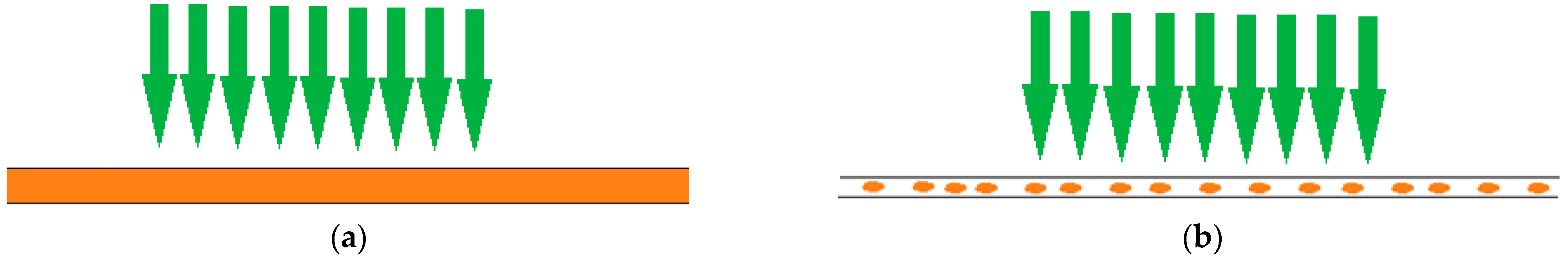
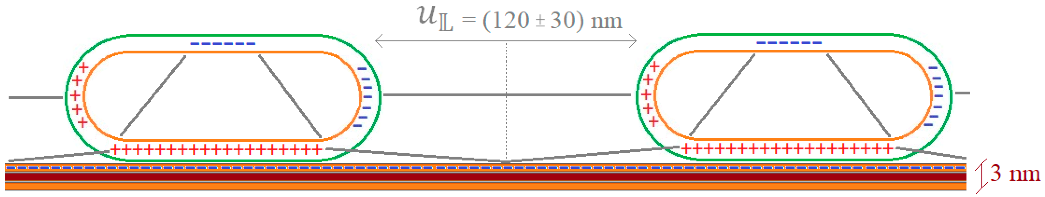
3.1. Considered System

Figure 4 and Figure 5 depict a simple system consisting of two pieces of borosilicate glass surrounded by air and joined together by a transparent glue. This is to serve as a thermal transducer. On the top and bottom sides of the smaller piece, gold nanorods are dislocated. Glass is prepared here due to its high transparency, facilitating heat to be produced within the system. On the top of the glassy domain (4), where the gold nanorods are dislocated, parallel laser beams are directed. Due to the great distance between them, some light penetrates the top and reaches the second, bottom gold surface.

3.2. Calculations of Energy Conversion Rate

Calculations from a total number of ${10}^{23}$ particles cannot be obviously accomplished due to the simulation time that would tend to infinity. This is why ${\mathbb{W}}_i$, ${\mathbb{W}}_j$, and ${\mathbb{W}}_{\mathbb{L}}$ are reduced and divided into 50 × 500 × 200 parts. The expected values are determined as ${d_s}_i=15\pm 3 \mathrm{n}\mathrm{m}$, ${d_l}_j=55\pm 8 \mathrm{n}\mathrm{m}$, and $u_{\mathbb{L}}=120\pm 30 \mathrm{n}\mathrm{m}$. As a function which describes polydispersity, Gaussian and Lorentzian distributions are selected. The boundaries are fixed as $3\times ∆{d_s}_i$, $3\times ∆{d_l}_j$, and $3\times ∆u_{\mathbb{L}}$.

Table 1. Parameters of gold nanorods.

General Parameter	Assumed Value
Expected size of nanorods, $d_s$	$15\pm 3 \mathrm{n}\mathrm{m}$
Expected length of nanorods, $d_l$	$55\pm 8 \mathrm{n}\mathrm{m}$
Interdistance,$u_{\mathbb{L}}$	$120\pm 30 \mathrm{n}\mathrm{m}$
Capping agent thickness, $d_g$	4 nm
Nanoparticle concentration, $\xi$	$(1.63\pm 0.13)·{10}^{21}{\mathrm{m}}^{-3}$

summarizes details of the considered nanoparticles, whereas

Table 2. Electrical properties for the utilized materials.

Permittivities		$\mathit{\lambda }=808 \mathbf{n}\mathbf{m}$	References
Air, ${\epsilon }_a$		1.011639	[29]
Glass, ${\epsilon }_{bg}$		2.281912	[30,31]
Glue, ${\epsilon }_{gl}$		2.400680	[32]
Polyelectrolyte, ${\epsilon }_{sur}$		2.274245	[4]
Gold nanoparticles	$\mathbb{r}\mathbb{e}$	−25.035329	[33,34]
	$\mathbb{i}\mathbb{m}$	1.564609

indicates electrical properties under 808 nm laser illumination.

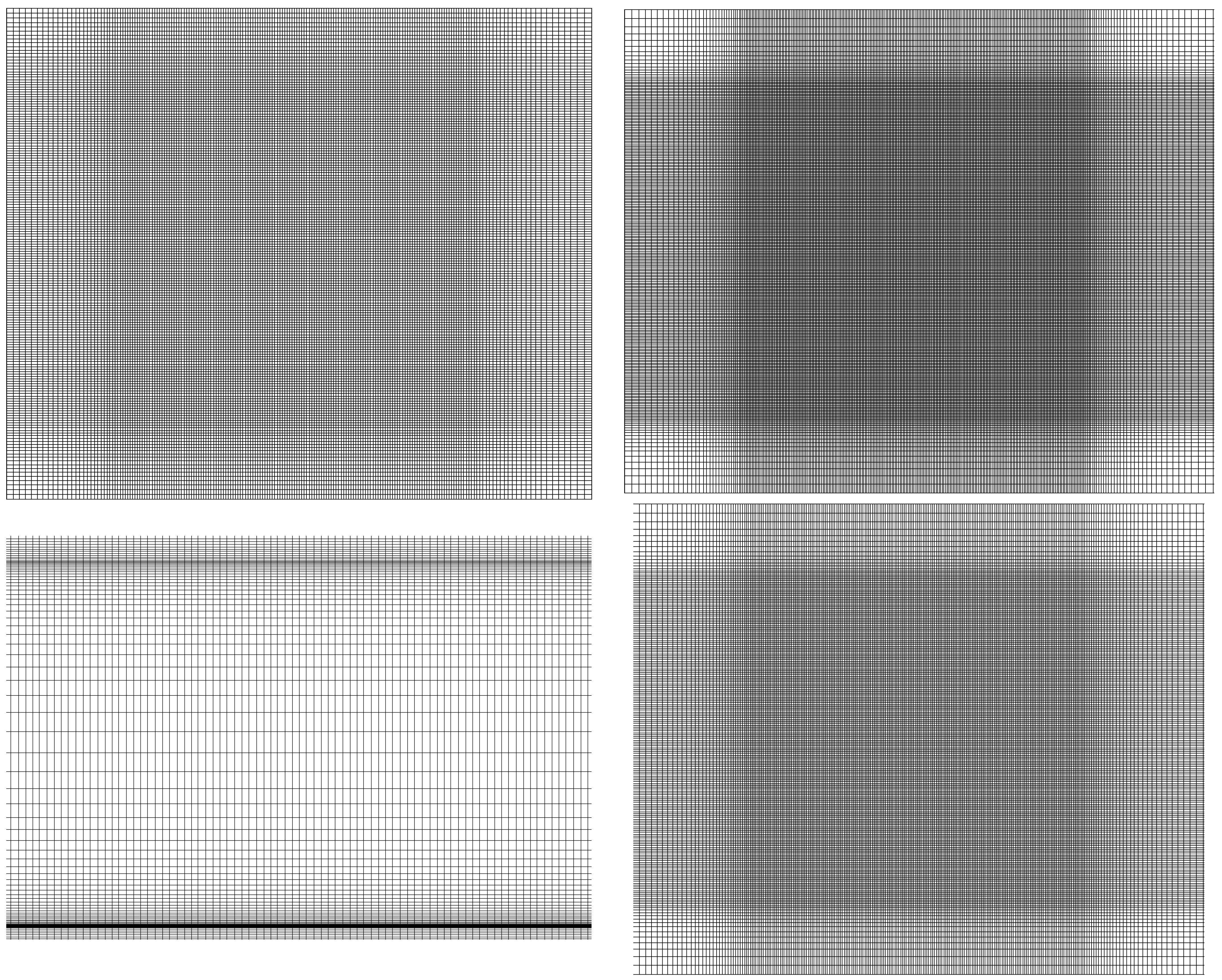
3.3. Numerical Model Implementations and Mesh Independences’ Proceedings

After determining the heat production rate generated by nanoparticles under laser irradiation, as described in Equations (11) and (13), we carried out numerical simulations based on the problem presented in Figure 4 and Figure 5, using the finite volume method (FVM). This computational technique discretizes the physical model into small control volumes and solves the governing equations at the centroids of these volumes. The calculations are run on the TrytonPlus supercomputer (CI TASK computing cluster, Gdansk, Poland, with the InfiniBand Fabric EDR 100 Gbps, fat tree topology network), which has 72 cores and supports the ANSYS Fluent software (versions 22.2 and 23.2). As outlined in the mathematical formulation section, we have treated Equations (2)–(7) relating to turbulent flows in three dimensions, using the standard $\mathbb{k}$-$\mathcal{E}$ turbulence model available in ANSYS Fluent software. For speed–pressure coupling, the SIMPLE algorithm is utilized, complemented by the PRESTO scheme for the spatial discretization of the pressure term, and a second-order upwind scheme for discretizing convective terms in the momentum and energy Equations (2)–(7). Under-relaxation factors of 0.3 for density and 0.5 for other parameters were used. Heat sources from Equations (11) and (13) were incorporated as boundary conditions on the considered surface, as indicated in Figure 4, using user-defined functions (UDFs) with the ‘DEFINE_PROFILE’ macro. UDFs dynamically distribute heat flux values over the surface under consideration, aligning them to the Gaussian distribution of the laser beam, as specified by Equation (17). These functions calculate the heat source term for each face of the control volumes during runtime, which enable us to model heat flux with spatial precision. The UDFs integrate the position vectors of the control volume faces and the laser beam intensity parameters to translate the physical beam profile into a precise heat source distribution during simulations.

Figure 6 reveals three meshes that were tested, providing minimal numerical error, using the Roacher and Richardson extrapolations [23,24]. A similar procedure is utilized for a time regime. The similar procedure is used for a time regime. The Roacher technique determines the continuum values of a given quantity $f_{qua}$ and highlights the relative and fractional error between different mesh or timestep results. This method is also intended for lower-order discrete values and is based on the following equation:

$$f_{qua}=f_{H=0}+C_1·H+C_2·H^3+\cdots$$

(35)

The continuum value $f_{H=0}$ for the second-order scheme employed in this work yields:

$$f_{H=0}=f_1+\frac{f_2-f_1}{{\left(\frac{H_2}{H_1}\right)}^{\theta }-1}$$

(36)

Similarly, for the three testing steps, Equation (25) is transformed into

$$f_{qua}=\frac{2^{\mathcal{n}}·f_1-f_2}{2^{\mathcal{n}}-1}$$

(37)

$$\mathcal{n}={\log }_2\left(\frac{f_2-f_3}{f_1-f_2}\right)$$

(38)

which enables the investigated value to be extrapolated with a specified error, e.g., the relative $\vartheta$ and fractional error ${\mathbb{E}}_1$ between two sets of data that follow

$$\vartheta =\frac{f_2-f_1}{f_1}$$

(39)

$${\mathbb{E}}_1=\frac{\vartheta }{{\left(\frac{H_2}{H_1}\right)}^{\theta }-1}$$

(40)

Furthermore, the grid convergence index ($GCI$) methodology has been introduced to indicate how far the error may change as the mesh is finer, which, for Richardson extrapolation, is defined by the $GCI$ parameter:

$$GCI=F^{\mathcal{S}}·\left|{\mathbb{E}}_1\right|=F^{\mathcal{S}}·\frac{\left|\vartheta \right|}{{\left(\frac{H_2}{H_1}\right)}^{\theta }-1}$$

(41)

where

• $\vartheta$—Relative error between two sets/values of data;
• $f_{H=0}$—Continuum value as if the mesh or time size equals zero;
• $C_{\mathrm{1,2},3,\dots }$—Constant or a function of the selected quantity that is other than $H$;
• $F^{\mathcal{S}}$—Factor of safety, here: 1.25.

3.4. Boundary Conditions

Boundary conditions allow the optimization of and reduction in the number of domains required to solve differential equations numerically. In this work, the system is assumed to be maintained under mixed conditions, incorporating both convection and radiation. To stabilize the computations and to omit the randomness and the initial zero problem, at starting point, a 1 μm/s velocity inlet and a pressure outlet along the gravity vector were assumed. Furthermore, due to the presence of an organic capping agent (citrate buffer), the application of the Marangoni stress to gold nanoparticles was necessary for managing the diffusive momentum flux:

$$\overrightarrow{X^{†}}\to \frac{d\stackrel{⃡}{\sigma }}{dT}·\mathrm{g}\mathrm{r}\mathrm{a}\mathrm{d}\left(T\right)$$

(42)

where the thermal coefficient of surface tension equals $-5.263 ·{10}^{-5} \mathrm{N}·{\mathrm{m}}^{-1}·{\mathrm{K}}^{-1}$ [31].

As a heat source, a 808 nm laser was positioned on the top surface of the platform where gold nanorods are localized. This wavelength was selected due to the similar absorbance of gold nanorods for air, water, and glue as a working medium, as explained in further sections. In the spatial regime, the laser beam followed a Gaussian distribution, presented in Formula (15), and the laser output power was set to $500 \mathrm{m}\mathrm{W}$. Higher powers were not considered due the power saturation, which would necessitate further modifications to the model. These would be subjects for future investigations. The laser-induced heat flux was delivered over a period of 70 s (irradiation time). After this time, the laser was off and the system cooled for 20 s.

Table 3. Material properties in the considered simulations.

Material	$\mathbf{Density}, \mathit{\rho }$ $\left(\mathbf{k}\mathbf{g}·{\mathbf{m}}^{-3}\right)$	$\mathbf{Specific} \mathbf{Heat} \mathbf{Capacity}, {{\mathit{c}}_{\mathit{p}}}_{\mathbf{e}\mathbf{f}\mathbf{f}}$ $\left(\mathbf{J}·{\mathbf{k}\mathbf{g}}^{-1}·{\mathbf{K}}^{-1}\right)$	Thermal Conductivity Coefficient, ${\mathit{k}}_{\mathbf{e}\mathbf{f}\mathbf{f}}$ $\left(\mathbf{W}·{\mathbf{m}}^{-1}·{\mathbf{K}}^{-1}\right)$	Dynamic Viscosity, $\mathit{\mu }$ $\left(\mathbf{P}\mathbf{a}·\mathbf{s}\right)$	References
Glass	$2124.9$	$779.74$	0.9245251 + 0.0004777689 · T $+9.178795·{10}^{-7}·T^2$	-	[33,34,35]
Glue	$1231$	$1100$	$0.50$	$0.30$	[36]
Gold nanorods	19,320	$129.81$	$317$	-	[37,38]
Air	$352.965·T^{-1}$	$1006.43$	0.004204762 $+7.242857·{10}^{-5}·T$	$7.29·{10}^{-6}$ $+4.0·{10}^{-8}·T$	[39,40,41,42]

displays thermal properties of the materials used to prepare the system, whereas

Table 4. Specified boundary conditions in the simulations carried out.

No.	Domain	Boundary Conditions
(1)	Bottom glass	$$\begin{gathered} T_o \\ h \\ ϵ \\ {S}_e^{\mathrm{f}} \end{gathered}$$	$$\begin{gathered} 297.15 \mathrm{K} \\ 13.6 \mathrm{W}·{\mathrm{m}}^{-2}·{\mathrm{K}}^{-1} \\ ϵ=0.957 \\ 0 \mathrm{W}·{\mathrm{m}}^{-3} \end{gathered}$$
(2)	Air	$L_{air}$	$0.01 \mathrm{m} (0.3937 \mathrm{i}\mathrm{n})$ (shell conduction)
		$S_e^{\mathrm{f}}$	$0 \mathrm{W}·{\mathrm{m}}^{-3}$
		$v_o$	$1 \mathsf{\mu }\mathrm{m}·{\mathrm{s}}^{-1}$ (at inlet)
(3)	Glue	$T_o$	$297.15 \mathrm{K}$
(4)	Top glass	$$\begin{gathered} S_e^{\mathrm{f}} \\ {T}_o \\ h \\ ϵ \end{gathered}$$	$$\begin{gathered} 1.07516·{10}^5 \mathrm{W}·{\mathrm{m}}^{-3} \\ 297.15 \mathrm{K} \\ 13.6 \mathrm{W}·{\mathrm{m}}^{-2}·{\mathrm{K}}^{-1} \\ 0.957 \end{gathered}$$
(5)	Gold slabs	${\stackrel{̿}{\delta }}_i$	$26.0 \mathrm{n}\mathrm{m}$
		$\frac{d\stackrel{⃡}{\sigma }}{dT}$	−$0.00005263 \mathrm{N}·{\mathrm{m}}^{-1}·{\mathrm{K}}^{-1}$
		${S_e^{\mathrm{n}\mathrm{p}}}_{Up}$	$4.71214·{10}^{11} \mathrm{W}·{\mathrm{m}}^{-3}$
		${S_e^{\mathrm{n}\mathrm{p}}}_{Down}$	$4.43412·{10}^{11} \mathrm{W}·{\mathrm{m}}^{-3}$
	System	$T_o$	$297.15 \mathrm{K}$
		$p_o$	1013.25 hPa

summarizes the assumed boundary conditions.

4. Results

4.1. Mesh and Time Independence Tests

Three meshes were tested to ensure the independence of the result to the mesh grid and time step size (Figure 6).

Table 5. Details of the applied meshes.

Parameter	Mesh 1	Mesh 2	Mesh 3
Mean mesh size	$0.1000 \mathrm{m}\mathrm{m}$	$0.0800 \mathrm{m}\mathrm{m}$	$0.0625 \mathrm{m}\mathrm{m}$
Maximum aspect ratio	$27.4834$	$30.7582$	$31.3168$
Mean volume cell	$6.2966·{10}^{-12} {\mathrm{m}}^3$	$5.6025·{10}^{-12} {\mathrm{m}}^3$	$3.4022·{10}^{-12} {\mathrm{m}}^3$
Orthogonal quality	$1.0$	$1.0$	$1.0$
Number of cells	$\mathrm{4,985,344}$	$\mathrm{8,324,230}$	$\mathrm{12,473,784}$

highlights details of all created grids. It should be added that the cells with maximum aspect ratio are located in the bottom glass (1) or in the glue zone (3) (see Figure 2). The maximum temperature in the entire system (max) and the average temperature of the top glass (4) were selected as quantity values for the Richardson extrapolation and GCI methodology, both in spatial and time regimes. The erroneous data are revealed in

Table 6. Parameters under Richardson and Roacher extrapolation proceedings after 30 s of illumination by a 1 W laser.

Extrapolated Error		Mesh 1–Mesh 2	Mesh 2–Mesh 3	${\mathit{t}}_{\mathcal{s}1}$–${\mathit{t}}_{\mathit{s}2}$	${\mathit{t}}_{\mathcal{s}2}$–${\mathit{t}}_{\mathcal{s}3}$
$\left|\vartheta \right|$	$T_{max}$	$0.14526\%$	$0.05424\%$	$0.007190\%$	$0.002261\%$
	$T_{av}$	$7.69209·{10}^{-5}\%$	$3.536·{10}^{-5}\%$	$0.001117\%$	$0.002921\%$
	$\left|\overrightarrow{v_{max}}\right|$	$0.7104\%$	$0.2263\%$	$0.2265\%$	$0.1396\%$
$f_{H=0}$	$T_{max}$	51.5538 °C	51.8365 °C	52.2260 °C	52.1884 °C
	$T_{av}$	25.7018 °C	25.7018 °C	25.7018 °C	25.7046 °C
	$\left|\overrightarrow{v_{max}}\right|$	$0.44305 \mathrm{c}\mathrm{m}·{\mathrm{s}}^{-1}$	$0.43170 \mathrm{c}\mathrm{m}·{\mathrm{s}}^{-1}$	$0.43267 \mathrm{c}\mathrm{m}·{\mathrm{s}}^{-1}$	$0.43268 \mathrm{c}\mathrm{m}·{\mathrm{s}}^{-1}$
${GCI}_{\left(fine\right)}$	$T_{max}$	$0.3721\%$	$0.1296\%$	$0.01027\%$	$0.003020\%$
	$T_{av}$	$1.970·{10}^{-6}\%$	$8.448·{10}^{-6}\%$	$0.001596\%$	$0.003901\%$
	$\left|\overrightarrow{v_{max}}\right|$	$0.01820\%$	$0.5407\%$	$0.3236\%$	$0.5290\%$
$f_{qua}$	$T_{max}$	51.8277 °C		51.7884 °C
	$T_{av}$	25.7018 °C		25.7018 °C
	$\left|\overrightarrow{v_{max}}\right|$	$0.43214 \mathrm{c}\mathrm{m}·{\mathrm{s}}^{-1}$		$0.43322 \mathrm{c}\mathrm{m}·{\mathrm{s}}^{-1}$

.

Given that the spatial errors were under 1%, the procedure was rerun for three timesteps—$t_{\mathcal{s}1}=5.0$, $t_{\mathcal{s}2}=2.5$, and $t_{\mathcal{s}3}=1.0 \mathrm{m}\mathrm{s}$. The resulting comparison suggests that time errors of up to 0.1% are feasible. The 2.5 ms mesh results, being spatially and temporally independent, are now advanced to experimental validation.

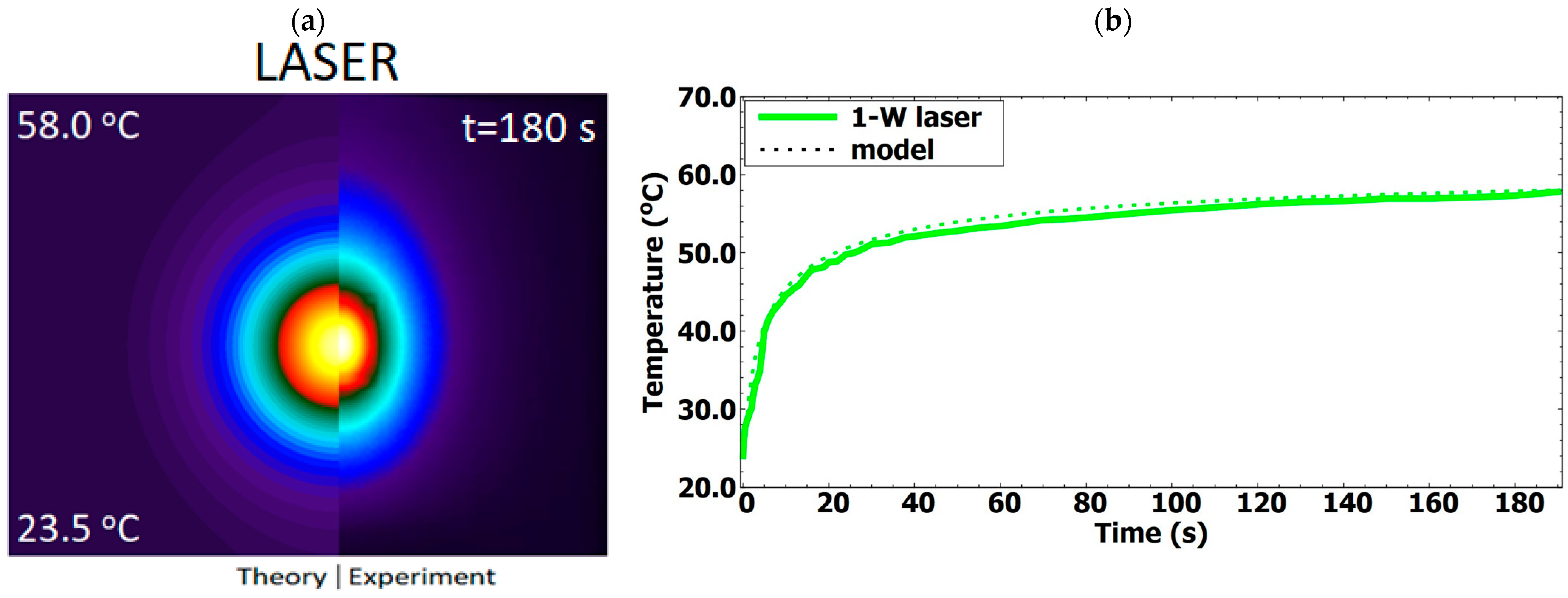
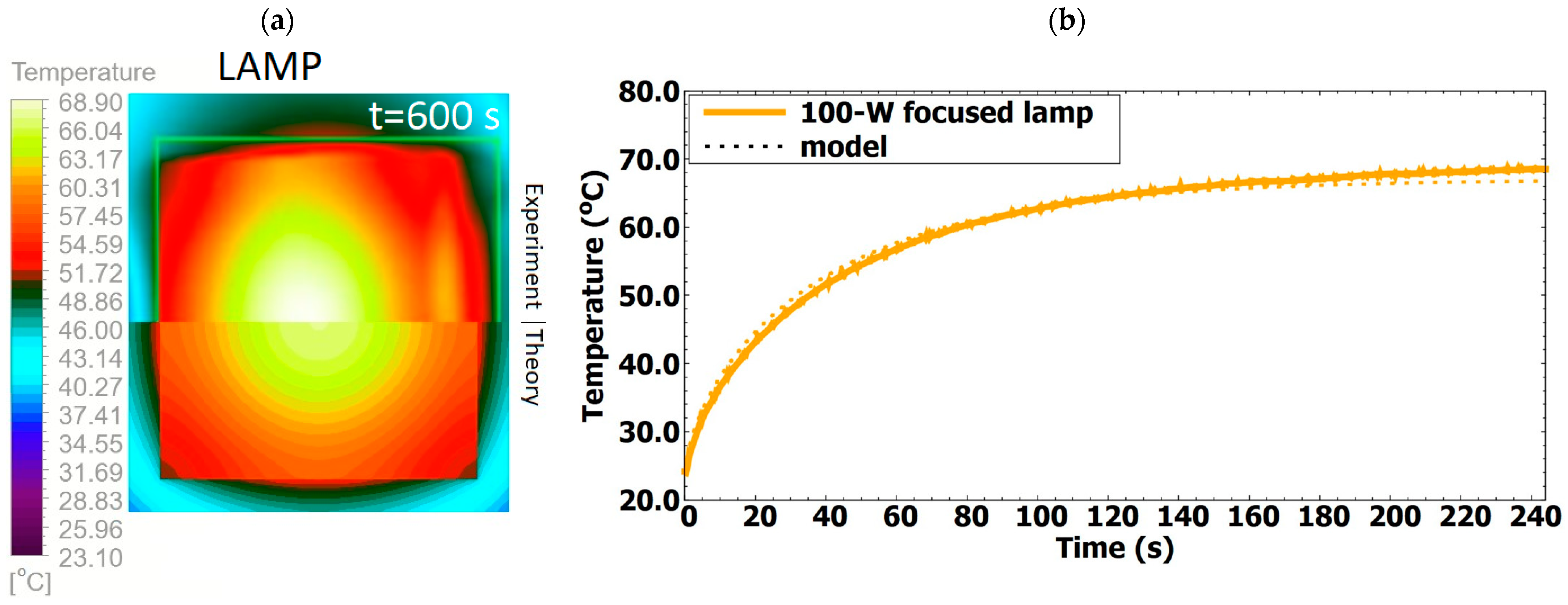
4.2. Experimental Validation

To validate the theoretical model, AuNRs were deposited on a glass substrate using the immersive layer-by-layer assembly technique according to the protocol reported in reference [3]. This technique allows for the immobilization of AuNRs on both sides of the glass substrate. After this step, a double glass cell was prepared by the scrupulously performing procedure reported in reference [4]. Then, the refractive index surrounding the AuNRs was consecutively varied from the front to the back sides of the AuNR substrate. Additional details can be found in reference [3].

Figure 7 depicts the absorption spectra of the AuNRs’ double cell, consecutively infiltrated with the glue (NOA-61) from the company Norland Products Inc. (Cranbury, NJ, USA), with a refractive index of 1.54 (from spectrophotometer PerkinElmer A Lambda 365 (Waltham, MA, USA)). The experimental optical behavior (continuous lines) agrees well with the theoretical model (dashed lines).

As may be noticed, the commendable agreement enables the ease of extension to almost the entire visible region and a part of the infrared region, up to 850 nm.

Figure 8 demonstrates the photothermal properties of the AuNR substrates upon laser light illumination, performed by using the optical setup and the experimental parameter reported in reference [3].

The results related to the temperature distribution, presented in Figure 8a, and the time–temperature profile (Figure 8b) demonstrate the full consistency between the experimental results and theoretical model. Validation of the model was conducted using a thermal imaging camera and the temperature field collected from the surface of the system under study [43].

As a consequence of this notification, this theoretical approach has been declared to be representative for the energy conversion and temperature distributions in this work. This decision is supported by the model’s reliability and accuracy in capturing the intricate interactions of light absorption and heat transfer dynamics. Moreover, $\lambda =808$ nm wavelength has been declared to possess a similar energy conversion for all three cases and only the materials’ properties and boundary conditions can affect heat transfer and the values of temperatures. Therefore, this laser is shifted to a further analysis.

Furthermore, the photothermal behavior of the AuNRs’ double cell was also investigated using a white light source, as outlined in the experimental procedure described in reference [4]. Experimental data are presented in Figure 9.

The model’s validity has also been raised and confirmed for the white-light lamp in [4] (Figure 9), notwithstanding the fact that the correlation is more pronounced for a single-laser approach. This can be attributed to the system’s irregularities, which pose a challenge to achieving ideal geometry. Consequently, optimization processes are deemed necessary and beneficial.

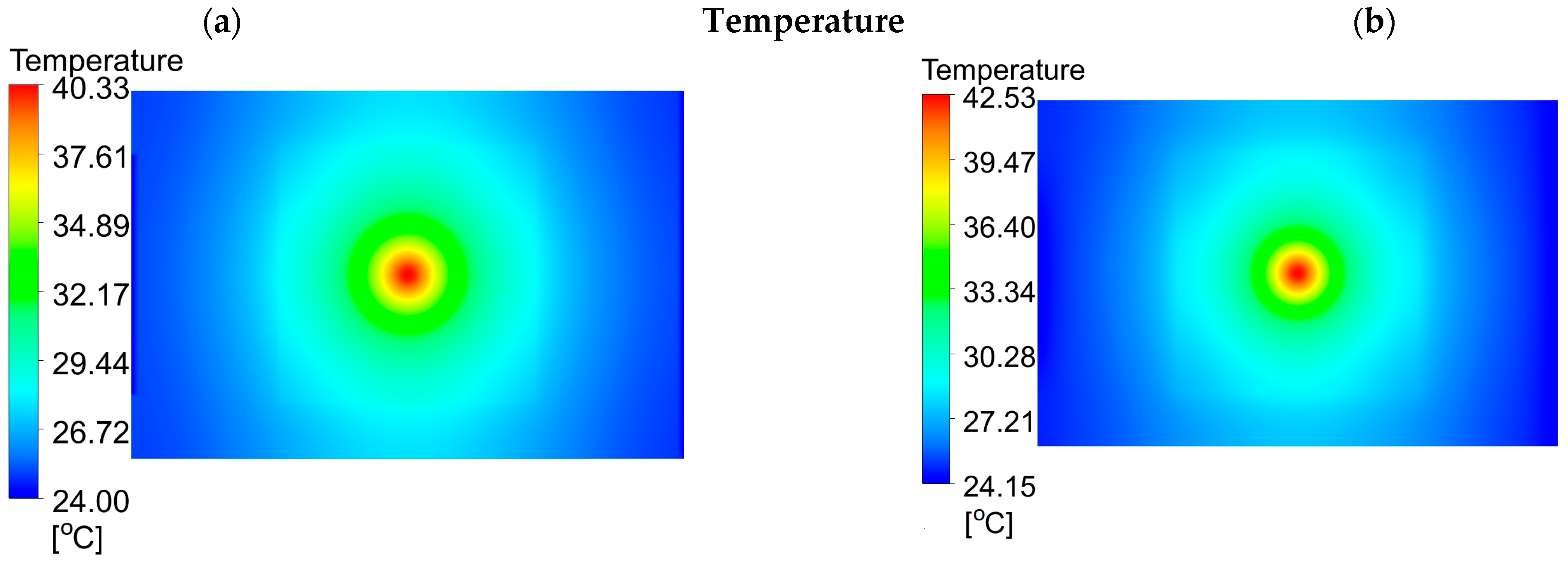
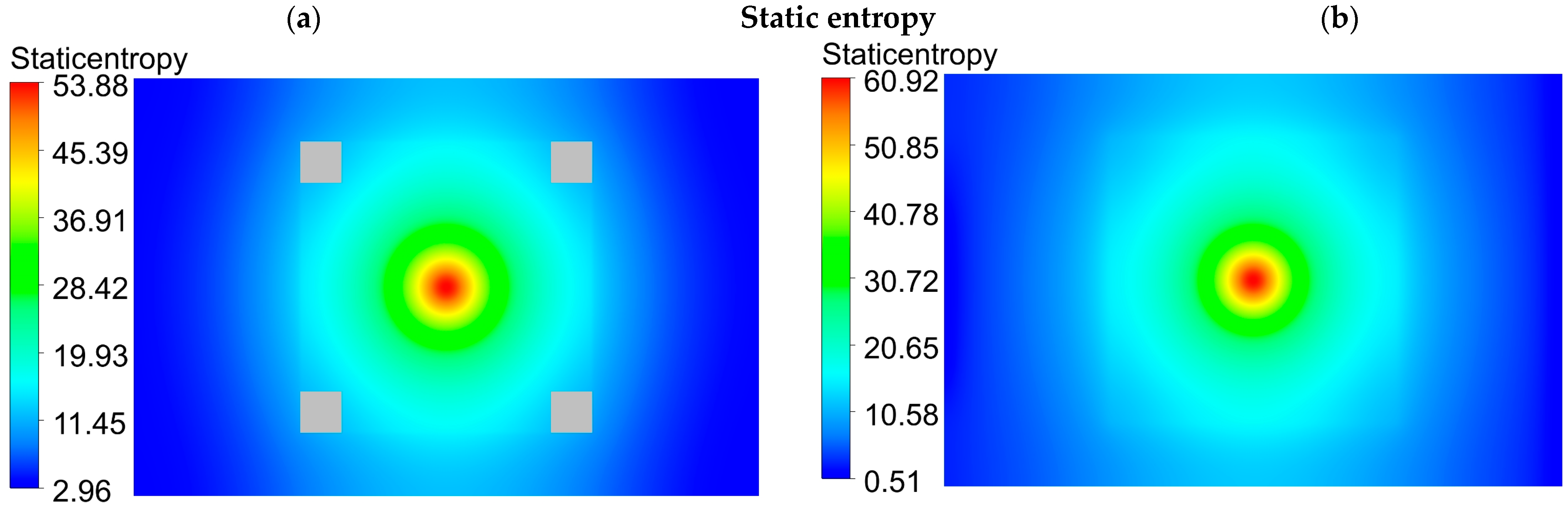
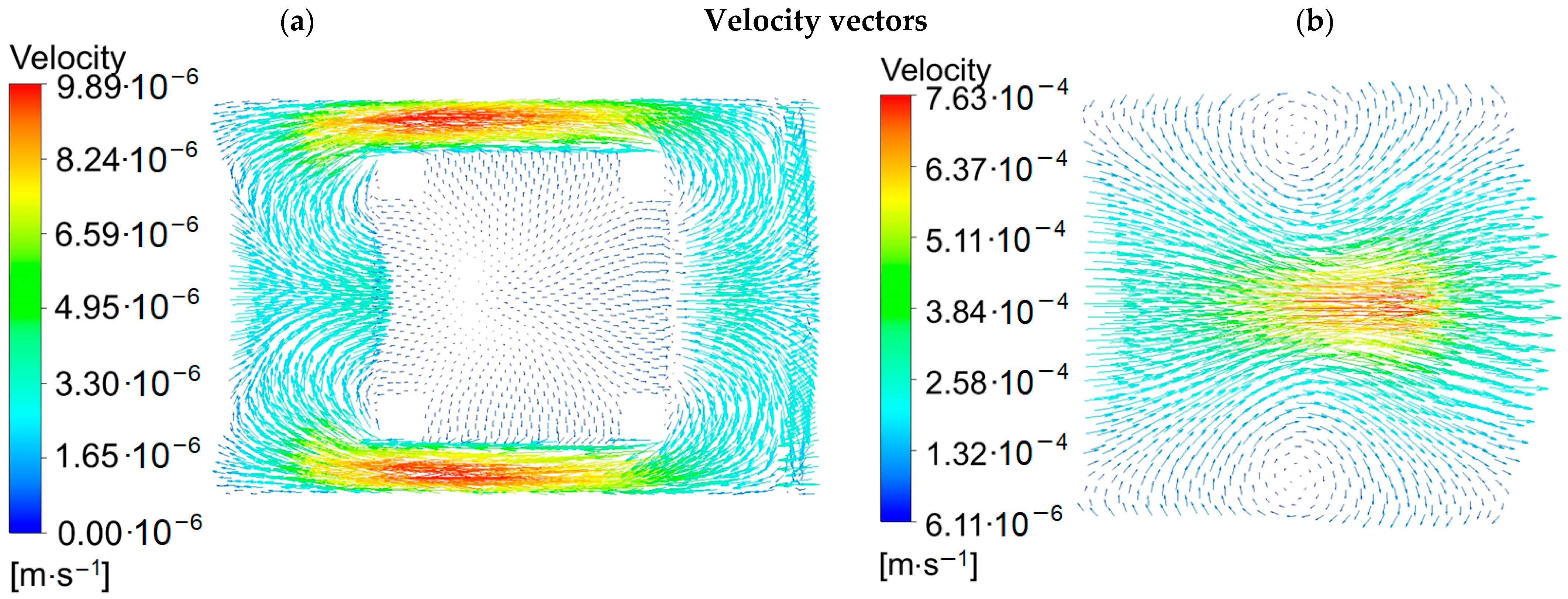
4.3. CFD Results for 0.5 W Laser Illumination

It should be noted that the thermal imaging camera analyzed the temperature field on the surface of the system for both the systems in Figure 8 and Figure 9. Consequently, the measurement tool employed does not permit a combined analysis of the temperature and velocity fields, and CFD calculations prove to be invaluable. The areas 5 μm above and 5 μm below the AuNRs’ platform of Figure 4 and Figure 5 were selected to present the results.

4.3.1. Heating Stage

Figure 10a,b exhibit the temperature after 70 s of light illumination, when the delivered heat begins to stabilize the temperature. Likewise, entropy contours are highlighted in Figure 11 and Figure 12 to control if the forced convection and inlet boundary conditions significantly changes the temperature contours. The left side (a) presents the plane 5 µm under the glass (4) domain in the nearly confined (closed) volume, whereas on the right side (b) results are considered 5 µm above the glass (4) domain, as exhibited in the free space. Accordingly, Figure 13 reveals fluid flow via the velocity vectors.

As can be observed, the maximum temperature reaches 40.3 °C below and 42.5 °C above the top glass (4), which is a promising temperature increase provided by a low operating laser power. In the real situations, higher powers are anticipated to raise the system’s maximum temperature significantly, as presented in Figure 8 and Figure 9.

4.3.2. Cooling Stage

Similarly, Figure 14, Figure 15, Figure 16 and Figure 17 illustrate the abovementioned results after 10 s of cooling when the whole system was reasonably close to being thermally equilibrated. In contrast to the heating stage, some values decrease by an order of magnitude as the temperature reduces. The velocity vectors, on the other hand, continue being horizontally oriented and their values have not been modified, whereas the maximum value of dynamic entropy slightly increases.

4.3.3. Time Responses

Time responses are strongly dependent on the boundary conditions and the complicity of the assumed mathematical functions. Some nanoscale results are based on Green’s or Gaussian functions, which are discussed in [7,25,26,27]. However, the presence of convection, which occurs in this work, encourages the use of numerical methods, which offer a similar effect.

Figure 18a depicts the maximum temperature, Figure 18b depicts the average temperature of the system, and Figure 18c represents the maximum velocity fluctuations over time. Results consider the cross-sections discussed in Figure 10, Figure 11, Figure 12, Figure 13, Figure 14, Figure 15, Figure 16 and Figure 17, located near the AuNRs’ platforms, at the bottom and top sides of the upper glass (4).

4.4. Discussion

The results in Figure 10 show a pronounced increase in temperature centered above and below the gold nanorod (AuNR) platforms, as expected due to the localized photothermal effect. The temperature contours suggest a strong radial distribution of heat from central hotspots corresponding to areas of direct laser irradiation. The maximum temperature recorded at these points corresponds to the known thermal properties of gold nanorods when subjected to laser radiation. It is also interesting to note that the temperature field decreases rapidly away from the center, indicating the efficiency of borosilicate glass’s thermal insulation properties. The uniformity observed in the temperature distribution suggests a homogeneous thermal conductivity distribution in the glass medium. Moreover, the colder regions around the heated zones confirm the role of air as an insulator, which is supported by the distinct boundary between the high-temperature regions and the surrounding area. During the cooling phase (see Figure 14), the temperatures in the core where laser irradiation occurred demonstrate a clear reduction, indicating efficient heat dissipation in the borosilicate glass and surrounding air. The uniform temperature gradient reflects the glass’s constant thermal conductivity and the air’s insulating role. The corresponding static entropy fields for the observed temperature fields are displayed in Figure 11 and Figure 15. As shown in Figure 11, the static entropy contours during the heating stage reflect the degree of disorder induced by laser heating for 70 s. Just above and below the AuNR platforms, there is a pronounced increase in entropy, indicating significant thermal activity. The central regions show the highest entropy values, revealing intense energy dissipation, which must be connected to the direct interaction of the laser with the AuNRs. As shown in Figure 15, during the transition to the cooling stage, the entropy levels decrease overall as the system loses thermal energy. However, the entropy distribution scheme remains similar, with the highest levels still concentrated around the central areas exposed to the laser. This region of constant high entropy suggests that AuNRs and associated regions retain heat longer or cool slower than surrounding materials. It should also be noted that the entropy does not immediately return to pre-heating values, suggesting a certain amount of thermal inertia or the presence of irreversible processes, even after the laser has been switched off.

As can be noticed in Figure 12 and Figure 16, the dynamic entropy values are approximately three orders of magnitude lower than the static entropy, indicating that, although fixed inlet boundary conditions stabilize calculations, they do not play a dominant role in forced convection and do not contribute to the total entropy and the general case. Indeed, the low dynamic entropy demonstrates that the thermal gradients and localized photothermal effects induced by laser irradiation on the AuNR platforms are the primary drivers of entropy generation rather than the fluid motion or inlet flow conditions. This observation holds for both heating and cooling phases, reaffirming that heat transfer mechanisms primarily drive the entropy scenario in this study. Moreover, the flow is observed for the glassy domain (4) from above, in the immediate vicinity of gold nanorods and only from the top. Due to the highly viscous forces, this effect is not visible in the confined area (bottom) where external flow and gravity cannot disrupt the boundary, and only free convection prevails inside. Furthermore, in the entire air domain, velocity vectors are oriented along the gravity force (Figure 13). However, the magnitude of vectors is distributed similarly to the temperature gradient and the temperature wave.

Nevertheless, vectors are distributed by the Gaussian laser profile from Equation (17), and residual flow is elevated due to the buoyancy forces and air density dependence, as presented in Table 3. Hence, competition arises between fluid weight, buoyancy forces, and the assumed laser profile. This competition is not observed at the same rate if gravitational forces act in parallel to the heat source as they do when they act perpendicular to it. This is because gravity forces attempt to retain the fluid while buoyancy forces strive to circulate it. Since viscous forces prevent the flow from entering the confined volume, velocity changes are governed only by natural convection in this region (see Figure 18c), contrary to the plane (top) where the system is exposed directly to the oriented flow. It may be noticed by studying the differences in the dynamic entropy contours (see Figure 12 and Figure 16). The topic is detailed in [44].

Furthermore, Gaussian (single-mode) and round (multi-mode) laser beams are distinguished by a similar radial temperature distribution, as seen in nozzles [45], where heat is delivered uniformly. Spatial distribution, characteristic of a Gaussian profile, however, offers an increase in the maximum temperature, although the energy conversion rate is on average comparable. It allows us to declare that a single-mode laser is sufficient to reach about 42.5 °C and 40.3 °C after 70 s of illumination (see Figure 18a) for a 0.5 W power and sparsely distributed nanoparticles if the surface is charged. Assuming the linear dependence between energy conversion rate and laser power, a two-watt near-infrared laser could potentially heat the system to reach 100 °C at this concentration. In reality, the energy conversion rate reaches a limit value that corresponds to the saturation temperature, as discussed in [46].

Additionally, produced heat appears to be distributed slowly due to low-diffusivity materials. This aspect is visible in Figure 18b, where both curves are similar. However, their tendencies are distinguishable due to the influence of natural convection and the magnitude of the velocity vectors. As long as the buoyancy effect intensifies heat transport, this influence is weak in the confined region where the region’s size (10 μm) allows the flow to increase only during a few hundred milliseconds. This is why the time responses of velocities distinguish considerably from one another, whereas maximum and average temperatures remain comparable. In turn, while the irradiation is turned off, the system enters a cooling stage. The dissipation of heat exceeds the input during this phase, leading to a rapid decrease in temperature, and velocity. The diminishing thermal input allows the system to return to a more disordered state—the interaction of temperature, velocity, and entropy describes the system’s dynamic response to a constant heat source (generated heat by AuNPs), demonstrating the complex balance between heat input, convective flow, and thermodynamic disorder. The complex interaction of several factors, including heat input, convective flow dynamics, and the system’s response to spatial constraints, generates entropy, as discussed in [47,48,49].

The observed changes in the presented results can be attributed to the system’s behavior during the simulation. The balance between heat input and output in the air medium influences the initial temperature rise. This phenomenon can be linked to the difference between the rate of heat absorption by the air and the dissipation rate. The velocity increases as the air near the wall heats up. This increase in velocity is accomplished by convective currents (free convection) induced by the temperature gradient.

The differences in parameter values observed between the air-exhibited area and the confined microscale volume can be attributed to the impact of spatial constraints on heat transfer and fluid dynamics. The restricted space in the confined microscale volume may result in enhanced heat conduction effects and a more localized influence of the heat source, resulting in different temperatures, velocities, and specific entropy patterns. Convective currents and heat dispersion, on the other hand, may operate more freely in the open area, where there are fewer spatial constraints, leading to higher values of temperature and velocity [50,51,52].

On the other hand, heat transfer in this case is not sufficiently fast to reach the steady state and a high temperature in less than one minute, which is indicated in tumors overheating. However, in this area, analyses of the material properties of biological structures and dedicated numerical calculations are necessary. Here, high-conductivity metallic sheets would reduce the effect of energy conversion, resulting in a low temperature increase. Therefore, glassy platforms with nanoparticles are declared only to convert energy and transduce it to the high-diffusivity materials, like metal sheets, that would distribute the heat throughout the entire system much faster than insulators. It is highly recommended studying this topic in the future. At this point, it is worth mentioning that in previous works, the authors have focused on comparing the CFD numerical model with simple geometry calculations [7,10]. For classical geometries, large compatibilities are obtained when using CFD tools with analytical methods. However, due to the need to develop complex geometries with the full Navier–Stokes equation as in the case of wind farms [53], it is necessary to take into account the advantages of CFD and perform simulations using this approach. Also, in the presented geometry and in the given physical phenomenon in this paper, there are reasons to use the CFD approach.

In addition, the work [54] compared three different theories of energy conversion into heat due to unique properties of gold nanoparticles (AuNPs), which may boost the efficiency in selected wavelengths. White-light-lamp-illuminated nanoplatforms with AuNPs were investigated via radiative transport, which were solved numerically using the discrete ordinates method (DOM). Optical boundary conditions were calculated analytically from data in the literature using three different approaches to describe the absorption coefficient, which defines the efficiency of the conversion. The selected approaches supported either the classical Maxwell model, Rayleigh approximation for nanostructures or the Mie–Lorenz theory for spheres. Likewise, in order to include substrate effect, a thin-film-adjusted model, developed by the authors of [4], was assumed. The results in [54] reveal a dozen Celsius-degrees increase for sparsely aligned gold nanoparticles, and vary significantly depending on the utilized model. Thus, the model presented in this paper is deemed the most appropriate compared to those mentioned above.

5. Conclusions and Perspectives

Although metallic nanoparticles can generally be modeled using standard transport equations described by exact differentials, they necessitate sophisticated mathematics, indicating the complexity of boundary conditions. According to this paper, metallic nanoparticles can be advantageous in applications where time is of the essence, such as cancer therapy and steam and bubble generation. The examined topic benefits from and encourages further research due to its promising temperature increase in energy or biomedical systems. The adopted model has been validated for a single-laser and a white-light source and could be further developed to accommodate more complex cases. Although NRs are not truly present, the interaction between NRs and light reflects the physical response, demonstrating that simple and well-known equations would unquestionably reduce simulation and CPU time. This work has also reported that a fixed inlet with a minimum velocity stabilizes calculations and improves results. Although it appears to be exaggerated and excessive, the gravitational forces overcome the inlet velocity after a few milliseconds, and the system follows the advisable conditions and results. According to the research, conduction is the most prevalent heat transfer mechanism. Despite the presence of viscous forces, their effect on overall entropy is minor. In addition, the low dynamic entropy observed compared to the static entropy indicates that the thermal effects of laser irradiation predominate over fluid dynamics in the entropy generation within the system. CFD models were compared with the analytical approach for solids in the works [7,10], confirming that CFD and analytical models give similar results for simple geometries. However, the CFD model used in this work is proven to be much more effective for complex geometries and fluid analysis [53], and therein lies the superiority of this tool over analytical solutions.

Additionally, the low dynamic entropy observed compared to the static entropy indicates that the thermal effects of laser irradiation predominate over fluid dynamics in the entropy generation within the system.

Our results reveal that the top plane of the gold nanorod platform exhibits a faster and more pronounced temperature and velocity response to irradiation than the bottom plane. In particular, the maximum temperature on the upper plane reaches around 43 °C after 70 s of irradiation, while the temperature on the lower plane increases gradually to around 38 °C. Both planes eventually exhibit similar behavior for the average temperature, reaching around 30 °C during the heating at 70 s. Velocity at the top plane quickly peaks at around 0.0008 m/s and remains at this level for 70 s, then rapidly decreases during the cooling phase. The theoretical results outline that even relatively low laser power values are sufficient to produce an impressive temperature increase. The maximum value in this work equals approximately $∆T\approx$ 18.5 °C and $∆T\approx$ 35.5 °C under a 808 nm illumination, respectively, for the 0.5 W and 1.0 W laser. However, challenges occur with heat transfer throughout the entire system. As long as convection and conduction can distribute heat, they cannot compete with changes in heat generation values. Consequently, low-thermal diffusivity and optically transparent materials, such as glass or epoxy, appear adequate for energy conversion, whereas other materials are preferable for intensifying heat transfer. The oriented flow, however, implies a heat wave whose front can affect and accelerate the achievement of high temperature on average using convective transportation methods.

Considering the present aspects of increased entropy generation with an increase in flow velocity, but an increase in heat transfer rates, there will be a need to perform an optimization task combining opposite objective functions. A multi-variant optimization approach similar to that described in the work of [55] is anticipated for further study.

References

1. Coyle, E.D.; Simmons, R.A. Understanding the Global Energy Crisis; Purdue University Press: West Lafayette, IN, USA, 2014. [Google Scholar]
2. Huang, Y.; Lee, C.K.C.; Yam, Y.-S.; Mok, W.-C.; Zhou, J.L.; Zhuang, Y.; Surawski, N.C.; Organ, B.; Chan, E.F.C. Rapid detection of high-emitting vehicles by on-road remote sensing technology improves urban air quality. Sci. Adv. 2022, 8, eabl7575. [Google Scholar] [CrossRef] [PubMed]
3. Petronella, F.; De Biase, D.; Zaccagnini, F.; Verrina, V.; Lim, S.; Jeong, K.; Miglietta, S.; Petrozza, V.; Scognamiglio, V.; Godman, N.P.; et al. Label-free and reusable antibody-functionalized gold nanorod arrays for the rapid detection of Escherichia coli cells in a water dispersion. Environ. Sci. Nano 2022, 9, 3343–3360. [Google Scholar] [CrossRef]
4. Zaccagnini, F.; Radomski, P.; Sforza, M.L.; Ziółkowski, P.; Lim, S.I.; Jeong, K.U.; Mikielewicz, D.; Godman, N.P.; Evans, D.R.; Slagle, J.E.; et al. White light termoplasmonic activated gold nanorod arrays enable the photo-thermal disinfection of medical tools from bacterial contamination. J. Mater. Chem. B 2023, 11, 6823–6836. [Google Scholar] [CrossRef] [PubMed]
5. Fang, X.; Wang, Y.; Wang, Z.; Jiang, Z.; Dong, M. Microorganism Assisted Synthesized Nanoparticles for Catalytic Applications. Energies 2019, 12, 190. [Google Scholar] [CrossRef]
6. Pontico, M.; Conte, M.; Petronella, F.; Frantellizzi, V.; De Feo, M.S.; Di Luzio, D.; Pani, R.; De Vincentis, G.; De Sio, L. 18F-fluorodeoxyglucose (18F-FDG) Functionalized Gold Nanoparticles (GNPs) for Plasmonic Photothermal Ablation of Cancer: A Review. Pharmaceutics 2023, 15, 319. [Google Scholar] [CrossRef] [PubMed]
7. Radomski, P.; Ziolkowski, P.; Mikielewicz, D. Energy conversion in systems-contained laser irradiated metallic nanoparticles—Comparison of results from analytical solutions and numerical methods. Acta Mech. Autom. 2023, 17, 540–549. [Google Scholar] [CrossRef]
8. Tofani, K.; Tiari, S. Nano-Enhanced Phase Change Materials in Latent Heat Thermal Energy Storage Systems: A Review. Energies 2021, 14, 3821. [Google Scholar] [CrossRef]
9. Mebared-Oudina, F.; Chabani, I. Revie on Nano Enhanced PCMs: Insight on nePCM Application in Thermal Management/Storage Systems. Energies 2023, 16, 1066. [Google Scholar] [CrossRef]
10. Radomski, P.; Ziolkowski, P.; De Sio, L.; Mikielewicz, D. Computational fluid dynamics simulation of heat transfer from densely packed gold nanoparticles to isotropic media. Arch. Thermodyn. 2021, 42, 87–114. [Google Scholar]
11. Mikielewicz, D. Hydrodynamics and heat transfer in bubbly flow in the turbulent boundary layer. Int. J. Heat Mass Transf. 2002, 46, 207–220. [Google Scholar] [CrossRef]
12. Ziolkowski, P.; Badur, J. A theoretical, numerical and experimental verification of the Reynolds thermal transpiration law. Int. J. Numer. Methods Heat Fluid Flow 2018, 28, 64–80. [Google Scholar] [CrossRef]
13. De Sio, L.; Placido, T.; Comparelli, R.; Curri, M.L.; Striccoli, M.; Tabiryan, N.; Bunning, T.J. Next-generation thermo-plasmonic technologies and plasmonic nanoparticles in optoelectronics. Prog. Quantum Electron. 2015, 41, 23–70. [Google Scholar] [CrossRef]
14. Sobhan, C.B.; Peterson, G.P. Microscale and Nanoscale Heat Transfer: Fundamentals and Engineering Applications; CRC Press: Boca Raton, FL, USA; Taylor & Francis Group: Abingdon, UK, 2008. [Google Scholar]
15. Cattaneo, M.C. A form of heat conduction equation which eliminates the paradox of instantaneous propagation. Compte Rendus 1958, 247, 431–433. [Google Scholar]
16. Radomski, P.; Zaccagnini, F.; Ziolkowski, P.; Petronella, F.; De Sio, L.; Mikielewicz, D. Heat Transfer of the Multicolor-Laser-Sources-Irradiated Nanoparticles in Reference to Thermal Processes. In Proceedings of the 36th International Conference on Efficiency, Cost, Optimization, Simulation and Environmental Impact on Energy Systems (ECOS), Las Palmas de Gran Canaria, Spain, 25–30 June 2023. [Google Scholar]
17. Bohren, C.F.; Huffman, D.R. Absorption and Scattering of Light by Small Particles; A Wiley-Interscience Publication: Toronto, ON, Canada, 1998. [Google Scholar]
18. Strutt, H.J.W. On the scattering of light by small particles. Lond. Edinb. Dublin Philos. Mag. J. Sci. 1871, 41, 447–454. [Google Scholar] [CrossRef]
19. Smoluchowski, M. On conduction of heat by rarefied gases. Ann. Phys. Chem. 1898, 64, 101–130. (In German) [Google Scholar]
20. Kreibig, U.; Vollmer, M. Optical Properties of Metal Clusters; Springer Series in Material Science; Springer: New York, NY, USA, 1995. [Google Scholar]
21. Yamaguchi, T.; Yoshida, S.; Kinbara, A. Optical Effect of the Substrate on the Anomalous Absorption of Aggregated Silver Films. Thin Solid Film. 1974, 21, 173–187. [Google Scholar] [CrossRef]
22. Fuchs, R. Theory of the optical properties of ionic crystal cubes. Phys. Rev. B 1975, 11, 1732–1740. [Google Scholar] [CrossRef]
23. Roache, P.J. Quantification of Uncertainty in Computational Fluid Dynamics. Annu. Rev. Fluid Mech. 1997, 29, 123–160. [Google Scholar] [CrossRef]
24. Richardson, L.F. The approximate arithmetical solution by finite differences of physical problems including differential equations, with an application to the stresses in a masonry dam. Phylosophical Trans. R. Soc. A 1911, 210, 307–357. [Google Scholar]
25. Domański, R. Laser Radiation—Solid-State Interaction; Polish Scientific-Technical Journals: Warsaw, Poland, 1990; pp. 130–220. ISBN 83-204-1383-4. (In Polish) [Google Scholar]
26. Carslaw, H.S.; Jaeger, J.C. Conduction of Heat in Solids, 2nd ed.; Oxford University Press: London, UK, 1959; pp. 50–132. [Google Scholar]
27. Romanchuk, B.J. Computational Modeling of Buble Growth Dynamics in Nucleate Pool Boiling for Pure Water and Aqueous Surfactant Solutions. Master’s Thesis, Division of Research and Advanced of the University of Cincinnati, Cincinnati, OH, USA, 2014. [Google Scholar]
28. Darbari, B.; Rashidi, S.; Esfahani, J.A. Sensitivity Analysis of Entropy Generation in Nanofluid Flow inside a Channel by Response Surface Methodology. Entropy 2016, 18, 52. [Google Scholar] [CrossRef]
29. Nisar, K.S.; Khan, D.; Khan, A.; Khan, W.A.; Khan, I.; Aldawsari, A.M. Entropy Generation and Heat Transfer in Drilling Nanoliquids with Clay Nanoparticles. Entropy 2019, 21, 1226. [Google Scholar] [CrossRef]
30. Zhang, L.; Bhatti, M.M.; Marin, M.; Mekheimer, K.S. Entropy Analysis on the Blood Flow through Anisotropically Tapered Arteries Filled with Magnetic Zinc-Oxide (ZnO) Nanoparticles. Entropy 2020, 22, 1070. [Google Scholar] [CrossRef] [PubMed]
31. Ziolkowski, P.; Badur, J. On Navier slip and Reynolds transpiration numbers. Arch. Mech. 2018, 70, 269–300. [Google Scholar]
32. Vial, A.; Laroche, T. Description of dispersion properties of metals by means of the critical points model and application to the study of resonant structures using the FDTD method. J. Phys. D Appl. Phys. 2007, 40, 7152–7158. [Google Scholar] [CrossRef]
33. Bengte, D.L. The Refractive Index of Air. Metrologia 1966, 8, 71–80. [Google Scholar]
34. Bansal, N.P.; Doremus, R.H. Handbook of Glass Properties; Academic Press: Cambridge, MA, USA; Materials Engineering Department Rensselaer Polytechnic Institute: Troy, NY, USA, 1986. [Google Scholar]
35. Zaitlin MP Anderson, A.C. Thermal Conductivity of Borosilicate Glass. Phys. Rev. Lett. 1974, 33, 1158–1161. [Google Scholar] [CrossRef]
36. Mark, J.E. Polymer Data Handbook; Oxford University Press: London, UK, 1999; Volume 131, p. 44. [Google Scholar]
37. Reddy, H. Temperature-dependent optical properties of gold thin films. Opt. Mater. Express 2016, 6, 2776–2802. [Google Scholar] [CrossRef]
38. Siegel, R.; Howell, J.R. Thermal Radiation Heat Transfer; McGraw-Hill Book Company: New York, NY, USA, 1972. [Google Scholar]
39. Engineering ToolBox. Air—Density, Specific Weight and Thermal Expansion Coefficient vs. Temperature and Pressure. 2003. Available online: https://www.engineeringtoolbox.com/air-density-specific-weight-d_600.html (accessed on 17 February 2023).
40. Engineering ToolBox. Air—Thermal Conductivity vs. Temperature and Pressure. 2009. Available online: https://www.engineeringtoolbox.com/air-properties-viscosity-conductivity-heat-capacity-d_1509.html (accessed on 17 February 2023).
41. Engineering ToolBox. Air—Dynamic and Kinematic Viscosity. 2003. Available online: https://www.engineeringtoolbox.com/air-absolute-kinematic-viscosity-d_601.html (accessed on 17 February 2023).
42. Fernández-Prini, R. Release on the Refractive Index of Ordinary Water Substance as a Function of Wavelength, Temperature and Pressure. J. Phys. Chem. Ref. Data 1998, 27, 761. [Google Scholar]
43. Koulali, A.; Ziółkowski, P.; Radomski, P.; De Sio, L.; Zieliński, J.; Mikielewicz, D. Single-Phase CFD Approach for Investingating Bacterial Inactivation and Heat Transfer in a Microchamber; Book of extended papers from XXV Jubilee Congress of Thermodynamics in Gdańsk (Poland), 11–14 September 2023; Gdańsk University of Technology Redaction: Gdańsk, Poland, 2023; pp. 167–174. [Google Scholar]
44. Koulali, A.; Abderrahmane, A.; Jamshed, W.; Hussain, S.M.; Nisar, K.S.; Abdel-Aty, A.H.; Yahia, I.S.; Eid, M.R. Comparative study on effects of thermal gradient direction on heat exchange between a pure fluid and a nanofluid: Employing finite volume method. Coatings 2021, 11, 1481. [Google Scholar] [CrossRef]
45. Piotrowicz, M.; Flaszynski, P.; Doerffer, P. Effect of Hot Spot Location on Flow Structure in Nozzle Guide Vane. IOP Conf. Ser. J. Phys. Conf. Ser. 2018, 1101, 012025. [Google Scholar] [CrossRef]
46. Patthew, P.; Garnett, B. Introduction to Metal-Nanoparticle Plasmonics; A Wiley–ScienceWise Publishing Co-Publication: Hoboken, NJ, USA, 2013. [Google Scholar]
47. Zhengdao, W.; Wei, Y.; Qian, Y. Numerical study on entropy generation in thermal convection with differentially discrete heat boundary conditions. Entropy 2018, 20, 351. [Google Scholar] [CrossRef] [PubMed]
48. Al-Kouz, W. MHD darcy-forchheimer nanofluid flow and entropy optimization in an odd-shaped enclosure filled with a (MWCNT-Fe3O4/water) using galerkin finite element analysis. Sci. Rep. 2021, 11, 2263. [Google Scholar] [CrossRef] [PubMed]
49. Drożyński, Z. Entropy increase as a measure of energy degradation in heat transfer. Arch. Thermodyn. 2013, 34, 147–160. [Google Scholar] [CrossRef]
50. Bejan, A. Fundamentals of Exergy Analysis, Entropy Generation Minimization, and the Generation of Flow Architecture. Int. J. Energy Res. 2002, 26, 1–43. [Google Scholar] [CrossRef]
51. Sciubba, E. Use of Exergy Analysis To Compute The Resource Intensity of Biological Systems and Human Societies. In Proceedings of the 12th Joint European Thermodynamics Conference, Brescia, Italy, 1–5 July 2013; pp. 268–273. [Google Scholar]
52. Jou, D. Entropy, entropy flux, temperature, and second law in extended irreversible thermodynamics. In Proceedings of the 12th Joint European Thermodynamics Conference, Brescia, Italy, 1–5 July 2013; pp. 211–216. [Google Scholar]
53. Flaszynski, P.; Wasilczuk, F.; Piotrowicz, M.; Telega, J.; Mitraszewski, K.; Hansen, K.S. Numerical simulations for a parametric study of blockage effect on offshore wind farms. Wind Energy 2023, 27, 53–74. [Google Scholar] [CrossRef]
54. Radomski, P.; De Sio, L.; Ziółkowski, P.; Mikielewicz, D. Heat Transfer in a Metallic-Nanoparticles-Contained System Using the Discrete-Ordinates and Thin-Film-Adjusted Models; Book of papers from XXV Jubilee Congress of Thermodynamics in Gdańsk (Poland), 11–14 September 2023; Gdańsk University of Technology Redaction: Gdańsk, Poland, 2023; p. 91. [Google Scholar]
55. Zuo, W.; Li, F.; Li, Q.; Chen, Z.; Huang, Y.; Chu, H. Multi-objective optimization of micro planar combustor with tube outlet by RSM and NSGA-II for thermophotovoltaic applications. Energy 2024, 291, 130396. [Google Scholar] [CrossRef]
Figure 1. Scheme of energy conversion calculations for (a) thin films and (b) nanoparticles.
Energies 17 02587 g001
Figure 2. Assumed electric field distribution (dipole configurations) for a 15-15-55 nm gold nanorod (orange color) capped by a 4-nanometer-thick citrate buffer (green color). Projections on the i ^ axis are marked by a violet color.
Energies 17 02587 g002
Figure 3. Scheme of the electrical field distribution with AuNRs deposited onto the PEL sandwiched functionalized substrate (side view). This reflects the mentioned name ‘AuNRs platform’.
Energies 17 02587 g003
Figure 4. Scheme and dimensions of the gold nanorod platform from side view (scale has not been saved).
Energies 17 02587 g004
Figure 5. Scheme and dimensions of the gold nanorod platform from top view (scale has not been saved).
Energies 17 02587 g005
Figure 6. Three discretized meshes employed in computations on both sides. Mesh at the bottom has been assigned to demonstrate theoretical results.
Energies 17 02587 g006
Figure 7. Experimental validation of the absorption spectra using a spectrophotometer for three different working media, ε h deposited on the 3 nm PAH-PSS polyelectrolyte. The structure of the capping agent, as an organic material, is difficult to predict theoretically without stochastic methods, and is conceived to explain visible discrepancies.
Energies 17 02587 g007
Figure 8. Experimental validation of (a) the temperature distribution and (b) time response from a thermal camera for a 1 W laser approach.
Energies 17 02587 g008
Figure 9. Experimental validation from a thermal camera of (a) temperature distributions and (b) time response for a white-light approach based on [4].
Energies 17 02587 g009
Figure 10. Temperature contours, according to Figure 4 and Figure 5. A distance of 5 μm under (a), and 5 μm above (b) the AuNR platforms (5) after 70 s of the laser illumination.
Energies 17 02587 g010
Figure 11. Static entropy contours, according to Figure 4 and Figure 5. A distance of 5 μm under (a), and 5 μm above (b) the AuNR platforms (5) after 70 s of the laser illumination. Gray color indicates places where glue has been dislocated.
Energies 17 02587 g011
Figure 12. Dynamic entropy contours, according to Figure 4 and Figure 5. A distance of 5 μm under (a), and 5 μm above (b) the AuNR platforms (5) after 70 s of the laser illumination. Gray color indicates places where glue has been dislocated.
Energies 17 02587 g012
Figure 13. Velocity vectors, according to Figure 4 and Figure 5. A distance of 5 μm under (a), and 5 μm above (b) the AuNR platforms (5) after 70 s of laser illumination.
Energies 17 02587 g013
Figure 14. Temperature contours, according to Figure 4 and Figure 5. A distance of 5 μm under (a), and 5 μm above (b) the AuNR platforms (5) after 10 seconds of cooling.
Energies 17 02587 g014
Figure 15. Static entropy, according to Figure 4 and Figure 5. A distance of 5 μm under (a), and 5 μm above (b) the AuNR platforms (5) after 10 s of cooling. Gray color indicates places where glue has been dislocated.
Energies 17 02587 g015
Figure 16. Dynamic entropy, according to Figure 4 and Figure 5. A distance of 5 μm under (a), and 5 μm above (b) the AuNR platforms (5) after 10 s of cooling. Gray color indicates places where glue has been dislocated.
Energies 17 02587 g016
Figure 17. Velocity vectors, according to Figure 4 and Figure 5. A distance of 5 μm under (a), and 5 μm above (b) the AuNR platforms (5) after 10 s of cooling.
Energies 17 02587 g017
Figure 18. Time responses of (a) maximum, (b) average temperature, and (c) magnitude of velocity vectors 5 μm above (top plane) (red color) and 5 μm under (bottom plane) (blue color) the glassy domain (4) of the AuNR platforms, respectively.
Energies 17 02587 g018