1. Introduction
Offshore wind is an abundant energy resource with significant environmental and economic benefits. When it comes to assessing the magnitude of wind produced over the sea compared to land surface, offshore wind outperforms due to it being less impacted by topographical influences like surface roughness and low turbulence [
1,
2]. Quantifying wind in the lowest part of the atmospheric boundary layer is a challenge due to the combination of forcing produced from friction and vertical motion due to heat over the surface that affect wind formation [
3,
4]. Compared to land, the ocean produces a larger amount of water vapor that is transferred into the atmosphere, and the heat budget also differs, which affects the atmospheric stability conditions [
5]. As a result of being strongly impacted by the atmospheric stability associated with turbulence exchange and interaction with the ocean waves, the offshore wind shear profile is often complicated [
2,
6].
The operational efficiency of offshore wind farms relies on highly accurate information, and thus high-quality measurements, of wind and waves, which is a challenge due to the lack of routine atmospheric measurements [
7,
8]. To fill the gap of inadequate measurements, numerical weather prediction (NWP) models are used to predict atmospheric conditions at fine spatial and temporal scales. While many current studies apply NWP models to predict wind for wind energy farms located both offshore and onshore, there are some challenges that have been identified, particularly for the offshore region [
9,
10]. Complexities arise due to land–ocean interactions, the formation of low-level jets, the dynamic nature of ocean–atmosphere waves, and high wind shear due to the stable boundary layer over the ocean as warm air from the land rapidly moves toward the relatively cold ocean water [
11,
12,
13,
14,
15,
16].
According to the Offshore Wind Market report 2023 edition [
17], the United States’ (U.S.) offshore wind energy project development and operational pipeline grew to a potential generating capacity of 52,687 megawatts [
18] in 2022. Further, a national goal set in March 2023 of 112,286 MW of offshore wind energy is expected to be in line with global growth patterns by 2050. The Mid-Atlantic Bight has recently seen heavy investment in offshore wind power farms, with most installations still ongoing or planned in the next few years, as of this writing [
19]. Offshore wind farms must be designed to withstand extreme weather including tropical storms, extreme wind/wave events, icy conditions, and extreme heat or cold. In addition, wind drought (very low wind occurrences) is an extreme condition that hinders the energy production capacity of wind farms [
20]. Given the plan by most NE U.S. states to move to 100% clean energy by 2040 to 2050 (Clean Energy States Alliance website, accessed September 2023), we expect increasing reliance on renewable resources in the near future. Climate assessment studies point to a potential future decrease in wind speed and wind power density for the offshore region of the NE U.S. [
21,
22,
23,
24,
25,
26], which could affect wind power generation reliability. Anticipating and, thus, reliably predicting such wind drought offshore conditions would be beneficial for the wind power industry and utility operators.
The efficiency of high-resolution hub height wind prediction for such events has not been extensively investigated. Moreover, due to the relationship between wind power density and cubed wind speed, small changes in wind speed prediction will lead to important changes in wind power density prediction. We investigated the performance of a high-resolution NWP model that can address the mentioned challenges, focusing on the U.S. Northeast Atlantic region. To apply a high-resolution mesoscale model suitable for predicting offshore wind at vertical height corresponding to the wind turbine hub level, we performed multiple sensitivity simulations using the Weather Research and Forecasting (WRF) [
27] model version 4.4. Our goal was to explore domain configurations with multiple nested domains, variations in the initial and boundary conditions, number of model vertical layers, and sea surface temperature fields.
While designing and analyzing the modeling experiments, the following questions were considered: What is the impact of the initial and boundary conditions, and number of vertical layers for the prediction of offshore hub height wind during anticyclonic conditions? How important is an accurate representation of the sea surface temperature (SST) field in the WRF to accurately depict the hub height wind? How is the wind power density affected by changes in the predicted hub height wind? These questions guide our assessment of the WRF model’s efficiency to accurately predict offshore wind speed over the Northeast U.S. cluster of wind farm lease areas. The long-term goal is to be able to accurately forecast conditions of wind extremes, on both sides of the spectrum, low and high winds that affect offshore wind turbine operations.
2. Materials and Methods
2.1. WRF Model Configuration
The WRF v4.4 model, which for many years has been a useful tool for operations and research [
27,
28,
29], is applied here with two different initial and boundary conditions and two-way nested domains with the finest domain having dx = dy = 600 m (
Figure 1). We chose the dynamic solver Advanced Research WRF (ARW), which uses a fully compressible, non-hydrostatic Euler equation and consists of a vertical coordinate system with terrain-following hydrostatic pressure [
27]. The ARW solver uses Arakawa C-grid staggering and is capable of formulating sub-grid scale turbulence in both coordinate and physical space [
27]. It provides velocity components (u and v), vertical velocity w, perturbation moist potential temperature, perturbation geopotential, and perturbation dry-air surface pressure as prognostic variables [
27]. Our project is a partnership with Eversource-Orsted focusing on the South Fork Wind Farm (SFWF) in the Northeast U.S. coast. The relatively high model resolution is chosen due to our collaboration with the research group that has developed the University of Connecticut’s large-eddy simulation model to depict wind turbines at a very fine scale [
30], using the WRF output as the initial and boundary conditions to the LES model.
For the domain selection, we considered available offshore observations covering the northeast U.S. coastline, especially near the South Fork Wind Farm (
Figure 1). The parent domain had an equal ratio of covering both land and ocean to observe the interaction of land and ocean with the atmosphere. The initial sensitivity tests revealed two datasets as the preferred ones for the initial and boundary conditions: the North American Mesoscale Forecast System (NAM) (Environmental Modeling Center, National Centers for Environmental Prediction, National Weather Service, NOAA, U.S. Department of Commerce) and the High-Resolution Rapid Refresh (HRRRv3) [
31] (
Figure 1 and
Table 1). The choice of the NAM and HRRR is based on the intention to deploy the WRF model operationally in the near future, and we needed to test modeling systems that can be used in forecast mode while offering sufficient high-resolution outputs. Both WRF configurations use the same physics parameterizations. The NAM/WRF configuration has three domains as the model had to dynamically downscale data from a coarse resolution of 12 km to 5.4 km, 1.8 km, and further 600 m. The HRRR/WRF configuration has two domains since downscaling needed to be performed from 3 km to 1.8 km and 600 m. We tested two sets of vertical levels for both initializations: (a) 56 vertical levels with 10 levels within 200 m and stretched above, and (b) 131 vertical levels with 21 levels (10 m intervals) up to ~400 m. For the rest of this article, we will refer to each configuration as the NAM/WRF and HRRR/WRF for simplicity.
We must mention here that there are also other components of the model configuration that could influence the modeled wind speed at the hub height, specifically the choice of the PBL parameterization scheme, data assimilation, convection scheme, and even model spin-up time. Our choice of the YSU PBL scheme, given our very high grid spacing that enters the terra incognita (
Table 1), was based on published work by Haupt et al. (2017) and Ching et al. (2014) [
32,
33]. Those studies have indicated that spurious numerically induced rolls are more apparent when applying a TKE-based PBL scheme like the Mellor–Yamada–Nakanishi–Niino (MYNN) [
34] than the YSU scheme. It was also beyond the scope of this paper to investigate all components influencing the offshore wind at the hub height. Our goal was to assess the initial and boundary conditions, SST, and vertical model layers.
Table 1.
WRF model configuration.
Table 1.
WRF model configuration.
| Numerical Weather Prediction Model | WRF v4.4 |
|---|
| Initial/boundary conditions | |
| Grid structure | Test 1 (with NAM):
5.4 km (D01), 1.8 km (D02) and 600 m (D03) | Test 2 (with HRRR):
1.8 km (D01) and 600 m (D02) |
| Vertical levels | Test 1: 56 vertical levels (Ptop = 50 hPa, 10 levels up to ~200 m) | Test 2: 131 vertical levels (Ptop = 50 hPa, 21 levels up to ~400 m) |
| Microphysics scheme | Thompson [35] |
| Planetary boundary layer | Yonsei University scheme, YSU [36] |
| Radiation scheme | Goddard for shortwave radiation [37]
RRTM for longwave radiation [38] |
| Land surface scheme | Unified Noah land-surface model [39] |
2.2. Offshore Observations
Historically, there have been more wind observations available up to the turbine hub height inland than offshore. With the increase in offshore wind farm developments in the Mid-Atlantic Bight, lidar buoys have been deployed to ensure the timely characterization of atmospheric condition. Our study area covers the cluster of leased wind farm areas in the Northeast U.S. (South Fork Wind and Revolution Wind;
Figure 1). There is no lidar buoy deployed in that area that provides free accessible data. To alleviate this observational gap, we used the Woods Hole Oceanographic Institution’s (WHOI) Air–Sea Interaction Tower (ASIT) [
40,
41]. Wind observations are available from anemometers located at 26 m AMSL (above mean sea level) and a single wind direction vane located at 23 m AMSL, as well as additional sensor data of air temperature, pressure, and relative humidity at 18 m AMSL and ocean temperature and salinity at 4 m BMSL (below mean sea level). More importantly, a lidar (WLS7-436) placed at the tower’s platform level provided wind observations up to 187 m AMSL [
42].
In terms of evaluating the model’s accuracy in forecasting offshore wind, one of the key factors is the SST, as it has a direct impact on atmospheric stability conditions. Though WRF can use the SST input from the relatively coarse initialization data, previous studies like Redfern et al. (2023) and Hawbecker et al. (2022) [
43,
44] have performed simulations with external SST inputs, which have a higher resolution compared to the initial and boundary conditions (ICs and BCs). They have observed that the differences in both temporal and spatial resolution between SST products have an impact on wind speed characterization, with higher resolutions tending to enhance model performance. We have compared the following SST datasets: the 0.01° Multiscale Ultrahigh Resolution (MUR) [
45], the 0.054° Office of Satellite and Product Operations (OSPO) analysis [
46], the 0.054° Operational Sea Surface Temperature and Sea Ice Analysis (OSTIA) [
47], the 1° Naval Oceanographic Office (NAVO) [
48], and the 0.02° Geostationary Operational Environmental Satellites (GOES-16) dataset [
49], to find the SST that is closer to the observations. As the externally available SST products have resolutions ranging from 0.1 degree to 1 degree, our tests showed that OSPO was closest to the observed SST, and we chose to use this product and compare with the SST values from the NAM and HRRR. Details will be discussed in
Section 3.3.
2.3. Statistical Evaluation Metrics
The statistical metrics of interest are systematic and random components of the model error (bias, root mean squared error (RMSE), centered root mean squared error (CRMSE)).
Table 2 lists the formulas for each error metric. We also calculated 95th percentile confidence intervals for each error metric through bootstrapping (10,000 bootstrap samples with random replacement).
2.4. Selection of Events
Previous studies performed over offshore regions like Kempton et al. (2010) [
50] presented multiple scenarios explaining the impact of synoptic-scale circulation on wind power production. They showed that high winds are found mostly at locations with the highest surface pressure gradients, with weaker winds observed at the core of the high-pressure system. According to the DOE Office of Energy Efficiency & Renewable Energy, a wind velocity at the turbine height between 6 and 9 mph (2.7–4 m/s) is a typical range needed to drive wind turbines (or 3 m/s according to Zeng et al., 2019 [
51]), but the duration of wind at that cut-in rate is equally important.
Self-Organizing Maps (SOMs) are used to objectively select cases that would be simulated with WRF. The SOMs algorithm, developed by Kohonen at al. (1995) [
52], is a type of unsupervised artificial neural network used for clustering data and performing pattern identification. SOMs create structured maps with contiguous nodes holding similar data based on the number of nodes/matrixes the user selects. To begin a SOM, initialization weight vectors are assigned to the connections/nodes with input vectors. The initialization process employs principal component analysis, which evenly distributes weights depending on the two greatest principal component eigenvectors of the input data [
53,
54]. Based on the Euclidean distance, nodes compete to claim input vectors and winners are selected upon minimum distance. The weight vectors of the winning node and its neighbors keep updating to match the input patterns and final maps are generated through multiple iterations [
54,
55,
56].
We have used an open-source Python package, minisom [
57], to create the maps. For the input data, we used the normalized (spatial anomaly, data were normalized by subtracting the mean from each array) 00z geopotential height field at 850 hPa over the year 2020 from HRRR 3 km data [
31]. The total number of input vectors was 366 and for the training, we used 1000 iterations. We have selected geopotential height as our input vector as it can provide valuable information regarding atmospheric circulation. Sensitivity tests with different SOM node configurations (
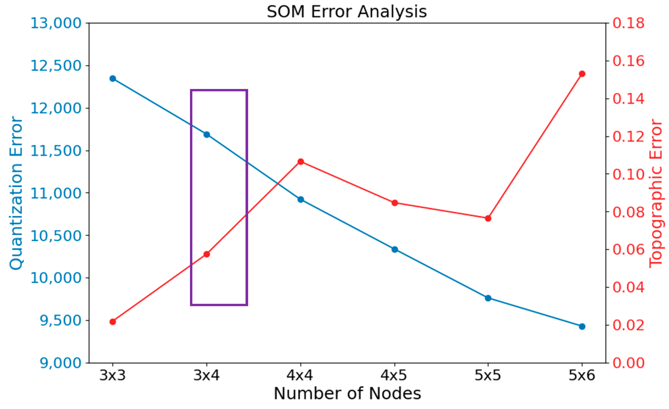
Figure 2) helped define a suitable number of nodes. We have compared the topographic error (TE) and quantization error (QE) for each combination. The QE is a measure of how well a map resembles the original data and is computed by averaging the distance between each input data point and its closest representative node on the map. As the number of nodes increases, the QE decreases. On the other hand, the preservation of spatial links between data points on a map is evaluated by the TE. The percentage of input data points for which the first and second best-matching nodes on the map are not neighbors is known as the topographic error, and it can be used to determine how well the map preserves the topological structure of the data. A lower topographic error indicates greater data topological retention [
54,
56]. Apart from the error values, we also considered the availability of sufficient sample size in each node and based on all these criteria, we have selected the 3 × 4 matrix with 12 nodes, where we have around 5% or more samples in each node (
Figure 3).
We selected two nodes (7 and 12) that are characterized by relatively weak forcing (
Figure 3). From both nodes, we have selected a total of six events that encompass winter, late spring, summer, and fall. The selected events are: from node 7: 22–24 January, 20–22 August, 18–20 October, and 8–10 November 2020; from node 12: 20–22 May and 15–17 June 2020. Each of the selected events had a high-pressure system present throughout the 48 h evaluation period (which excluded a 12 h model spin-up time) of the simulated event. Additionally, the persistence of the high-pressure system did not extend beyond the event period.
Regarding the high-pressure system location and occurrence time, we have consulted the surface analysis synoptic maps produced by NOAA’s Weather Prediction Center (
Figure 4) to confirm our SOM results. According to the synoptic maps, a high-pressure system originated further south over land, moved toward the Northeast Atlantic with 1032 mb highest pressure recorded at the system’s core (near Martha’s Vineyard) on 23 January 03 UTC. The wind speed was already lower than 5 m/s and the presence of the high pressure reduced it to around 3 m/s. The system continued to stay on the Atlantic coast, further north from Martha’s Vineyard throughout the event. For the May event, a persistent high-pressure system with 1032 mb central pressure is observed near Martha’s Vineyard throughout the event that took place on 20 May. The core of the anticyclone is positioned over the New England coast, where the wind speed decreases below 5 m/s (
Figure 4, 21 May 2020, 12 UTC). On 15 June, a high-pressure system with the highest recorded pressure of 1029 mb was positioned over the Great Lakes, with its extension influencing the location of the ASIT tower. Like the May event, a high-pressure system reaching 1017 mb was recorded on 21 August over the New England coast. The anticyclone is not as well organized as the May one, and the wind speed at the hub height did not exhibit the same decrease as shown in the wind speed time series that follow in
Figure 5. The wind speed decrease for the May event was about 8 m/s within 18 h, while for the August event, the decrease is about 5 m/s within 9 h (according to the time series presented in
Figure 5). A high-pressure system had been established over New Jersey by the onset of 18 October. Characterized by a robust core with a pressure of 1028 millibars, this system gradually shifted inland before progressing northward toward the North Atlantic region over the course of 18 and 19 October. The wind speed reached approximately 7.5 m/s on 18 October, but over the subsequent two days, it either remained below or hovered close to the cut-in threshold of 3 m/s. On 8 November, a well-organized high-pressure system with a peak pressure reading of 1029 mb was located over Pennsylvania, influencing the New England coast. The anticyclone moved east and over the Atlantic. During all these high-pressure systems, the ASIT tower observed a decrease in wind speed and a shift in wind direction for five of the systems.
3. Results and Discussion
In the following sections, we examine the performance of the various WRF configurations for sensitivity to the initial and boundary conditions, vertical levels, SST inputs, and influence on the prediction of wind power density.
3.1. Influence of Initial and Boundary Conditions
In this section, we discuss the hub height wind prediction for the six anticyclones due to the influence of the initial and boundary conditions. We have created time series plots of wind speed and wind direction at the closest available observation height of the wind turbine hub height (
Figure 5). The wind turbine hub height is 140 m AMSL (Dr. Astitha’s personal communication with Orsted, July 2023, site under construction), and we performed model evaluations at the lidar height that is closest to the hub height by interpolating the model to 147 m (ASIT tower lidar measurement height).
A major concern when conducting NWP simulations at grid spacing below ~1 km is the impact of the turbulence gray zone or the terra incognita [
58]. According to Rai et al. (2019) and Haupt et al. (2023) [
59,
60], the planetary boundary layer depth is the maximum limit of the terra incognita, meaning that horizontal spacing smaller than the boundary layer depth (but greater than around 100 m) is likely to produce fictitious secondary structures. For five out of six events (22 January, 20 May, 20 August, 18 October, and 8 November), the modeled PBL height at the location of the lidar buoy was nearly always lower than the horizontal grid spacing of 600 m (
Figure 6). Such an outcome supported findings from previous studies that showed no impact of the terra incognita when the PBL height is less than the horizontal grid spacing (Δx) but greater than 100 m [
59,
60] and provided confidence in our use of the 600 m gridded domain results.
The time series plots highlighted that both model configurations for the six different anticyclonic events captured the temporal evolution of wind speed at the hub height quite well (
Figure 5). Both model configurations struggled to capture the November event, which exhibited a steady upward trend of wind speed, though the NAM/WRF reached the peak at the very end of the simulation. Also, there was a sudden and frequent shift in wind direction, which prevailed from the northwest, but as wind speed dropped, the wind direction changed to become southward, ultimately settling into a southwesterly direction over time. Neither model could capture the clear westerly wind seen in the observations. In the month of January, initially, the predominant wind direction was from northwesterly to westerly, which gradually shifted to southwest because of the high-pressure system’s movement. Toward the end of the event, the wind direction reverted to northwest due to the influence of another high-pressure system developing further inland on the west. Both model configurations struggled to predict the first shift in the wind direction, but the HRRR/WRF managed to obtain the second one. In the May event, the wind was initially northeast and then shifted to a south–southeasterly direction due to the influence of the transition of high pressure. The models captured the transition very well. Like the May event, wind during the October event was initially coming from the northeast and transitioned between easterly to south-easterly and the HRRR/WRF performed better to capture the transition. In June, a northeast wind was predominant, which the models represented accurately. Finally, during the August event, winds were predominantly south–southwesterly, briefly shifting to northwesterly at the end of the event. Particularly, during the drop in the wind speed, the HRRR/WRF tended to portray the change in the wind direction closer to the observations.
The hub height winds for the six anticyclones were, for the most part, below the rated power wind speed for the South Fork wind farm, which is ~12 m/s (Dr. Astitha’s personal communication with Orsted, September 2023). This is the wind speed that the wind turbine will start producing its maximum constant power (or rated power) until, and if, the wind reaches a cut-out speed (varies by turbine). There are many consecutive hours in the individual six 48 h events, where the wind power generation would be highly variable (from the cut-in speed until 12 m/s) or zero (when the wind is less than the cut-in wind speed) (
Figure 5). According to the New York State Wind Energy Guidebook [
61], typically, wind turbines start producing electricity at wind speeds of about 6.7 mph (3 m/s), which is the value we used in our study. The wind turbine’s performance would be hindered when faced with reduced wind speeds, such as during the high-pressure systems we have analyzed, and being able to forecast them well in advance would be essential for wind farm operators and power utilities.
The performance of the HRRR/WRF was significantly better than the NAM/WRF for the May, August, and October anticyclones regarding RMSE and CRMSE (
Figure 7). Note that we used CRMSE to determine the discrepancies between the modeled and observed values that are due to random processes, and hence difficult to reduce. The May and August cases were very similar in the geographic positioning of the high-pressure system, which the HRRR/WRF captured better than the NAM/WRF. The systematic error (mean bias) for both cases was not statistically different between the two model configurations, pointing to no obvious change that would impact the statistical performance. For the January, June, and November events, the NAM/WRF was statistically better than the HRRR/WRF for RMSE (overall error). The January and June events share a similarity in terms of the timing of the high-pressure systems passing by and for both events, the NAM/WRF performed statistically better than the HRRR/WRF in terms of systematic error. Overall, the initial and boundary conditions played an important role for the WRF hub height wind prediction, with no clear indication about one preferred set of initial conditions that worked best for all simulated cases. We should note here that the NAM/WRF configuration had one extra nested grid compared to the HRRR/WRF domain setup, which likely contributed to some variation in the 600 m domain simulated wind speed. In general, the NAM/WRF and HRRR/WRF were capable of describing the low wind speed occurrences, with some under-prediction of higher winds, and difficulty in depicting the hub height wind speed increase (but still below the rated wind speed) during the November anticyclone. We further investigated the NAM/WRF and HRRR/WRF model performance differences as related to the vertical model levels, SST, and wind power density in the next sections.
3.2. Influence of Model Vertical Levels
We increased the vertical levels up to 400 m and added more levels within the boundary layer to investigate the impact in the prediction of the hub height wind speed. Bootstrapping confidence intervals for all combinations helped with the assessment of statistical improvement. The HRRR/WRF showed less varied PBL heights between simulations with 56 vertical levels versus 131 vertical levels compared to the NAM/WRF (
Figure 6). For all events, there was no statistically significant change due to adding more vertical levels within the lower boundary layer (
Figure 7). The confidence intervals clearly showed that the influence of the initial and boundary conditions was more important compared to adding more vertical levels (
Figure 7). These results underscored that increasing the vertical resolution did not systematically improve the prediction capability of each model configuration for these six cases.
3.3. Impact of SST
The sea surface temperature plays a critical role in the ocean–atmosphere interaction processes through vertical turbulent exchanges of momentum, heat, and moisture [
62]; thus, we assessed its impact on wind prediction capability. To this end, we evaluated two SST products at the observation location. We compared the model SST (NAM and HRRR), and five external SST datasets (OSPO, OSTIA, MUR, NAVO, and GOES-16) with the ASIT observation (as mentioned in
Section 2.2), to find the SST input that was closest to the observations. We decided to use the 5 km OSPO SST product as it best represented the observed SST (
Figure 8). The OSPO product has incorporated data from multiple sources, including satellite imagery and in situ measurements from ships and buoys, to provide accurate and detailed information on the SST across the region, while having good coverage over the Northeast U.S. [
63].
The SST time series revealed cases where (a) there was substantial deviation in the model SST magnitude compared to the observations, and (b) there was available high-resolution SST that matched the observations (
Figure 8). Therefore, of the six anticyclone cases, we selected the May, October, and November cases to further investigate the impact to the hub height winds from a better SST input (
Figure 8). For the August case, the SST from OSPO was close to the NAM and HRRR SST. For the January and June case, the ASIT tower did not provide SST data. We decided to use the HRRR initialization and 56 vertical levels, as the SST from the HRRR/WRF exhibited greater deviation from the observations (blue line in
Figure 8), and the 131 vertical levels did not significantly improve the results. The change in the SST input from the HRRR/WRF to the HRRR/WRF with OSPO for these three simulations did not significantly change the hub height wind speed prediction (
Figure 9). The simulation with OSPO SST tended to correct the time series of the wind and bring it closer to the observation during the period of descending wind, while it tended to increase the under-prediction during the period of rising wind for both the May and November cases. Meanwhile, for the October case, the simulation initially exhibited overprediction, but as the event progressed, its performance gradually approached that of the one without any external SST input.
3.4. Wind Power Density Prediction
From the previous sections, the conclusion was that the initial and boundary conditions exhibited the largest influence on the hub height WRF wind prediction. The NAM/WRF and HRRR/WRF configurations were able to capture low wind speed occurrences during the presence and movement of anticyclones, providing confidence that the model is capable of reliably predicting such wind drought occurrences. Even though we selected similar types of weather patterns over the Northeast U.S. (anticyclones with low wind), there was no single configuration that performed best for all cases. Naturally, the next question was whether a similar significance would apply to the prediction of offshore wind power density, given that wind power is based on cubic wind speed.
The calculation of the wind power density (WPD) [
23,
26,
64,
65], which represents the hypothetical wind power content of atmospheric flow, is shown below.
where ρ is the air density (1.207448 kg/m
3), and V is the wind speed in m/s. The unit of WPD is W/m
2. The calculation of the air density included a correction for elevation [
65,
66]:
).
For the selected cases, the hub height wind speed did not reach the rated speed of 12 m/s, except for a few hours in May and August (
Figure 5). This indicated the importance of weakly forced events that produce a low wind speed and how they might influence offshore wind energy production. We plotted time series of the WPD for each event (
Figure 10) to investigate the impact of wind speed biases on wind power. As the WPD is proportional to the cubic wind speed, a small deviation in the modeled wind from observations can have a great impact on wind power. This feature was more pronounced for higher wind speeds, as expected (May and August cases,
Figure 5 and
Figure 10).
The statistically significant difference between the WRF model configurations followed the same patterns as for the hub height wind speed for the individual events (
Figure 11). For the May and August anticyclones, the HRRR/WRF had a statistically lower RMSE and CRMSE compared to the NAM/WRF for the WPD. For October, the HRRR/WRF had a statistically lower BIAS compared to the NAM/WRF. For the January, June, and November anticyclones, the NAM/WRF showed better error statistics, not consistently for the same metrics though. When testing the confidence of all events together, the HRRR/WRF model configuration had a significant low model and random error (RMSE and CRMSE) compared to the NAM/WRF, while the mean bias did not exhibit any significant difference. As with the hub height wind speed, the difference between vertical levels was insignificant for the WPD error metrics (
Figure 11). The mean values of all statistical metrics for the wind speed and WPD are provided in
Appendix A Table A1 and
Table A2.
4. Concluding Remarks
The main objective of this study was to investigate the influence of the initial and boundary conditions (NAM versus HRRR), number of vertical layers (56 versus 131), and SST (NAM/HRRR versus OSPO) on the WRF prediction of the offshore wind speed and wind power density. We explored the impact on the hub height wind prediction over the Northeast U.S. cluster of wind farm leased areas for anticyclones that coincide with low wind speeds and, thus, underproduction of wind energy. The only available offshore measurements at the time of the study came from the WHOI’s ASIT tower, which was adjacent and not directly inside the intended area of the offshore wind farm. This resulted in configuring the WRF modeling domains to include the tower location for model evaluation purposes.
We used SOMs to objectively select events that shared similar synoptic-scale conditions. We selected events of a similar type, originating from the same SOM node, that exhibited relatively weak winds coming from similar directions (northwesterly winds for two of the events under node 7 and northeasterly winds for the events under node 12 and one of the events under node 7). The maps also aided in identifying events with relatively weak forcing due to the regional pressure gradient, which translated in wind below the wind turbine rated wind speed limit. As the rated wind speed represents the operational conditions of the wind farm, it is very important for NWP models to accurately predict events with weak forcing when they are persistent in time.
Overall, the performance of the WRF model in predicting offshore wind at the hub height during the influence of anticyclones was primarily influenced by the initial and boundary conditions. Adding model vertical levels did not change the model performance significantly and consistently. Another important factor to consider was the SST field that could impact the atmospheric stability and air–sea fluxes, as variations in the SST affect the stability of the marine boundary layer and thus the generation of offshore winds. The OSPO SST was closer to the actual observed SST for three cases and corrected part of the wind profile for two of the selected cases (May and November), but it did not provide any significant improvement in the error statistics.
There was not a single model configuration that consistently gave statistically better hub height wind speed predictions, and when the wind speed translated to wind power density, the statistics remained the same. This was possibly the result of the limited set of anticyclonic cases, which did not permit the generalization of the conclusion for or against a particular set of initial and boundary conditions. Individually, the wind power density was better predicted by the HRRR/WRF for the May, August, and October anticyclones, while the NAM/WRF had better error statistics for the January, June, and November events. The HRRR/WRF configuration showed a significantly lower RMSE (216–242 W/m2) and CRMSE (180–201 W/m2) compared to the NAM/WRF, when we considered all six events together. Our work underscored that for predicting offshore wind resources, it is important to evaluate not only the WRF predictive wind speed, but also the connection of wind speed to wind power. The long-term goal of this project is to deploy WRF operationally for the NE U.S. wind farms by choosing the best potential configuration. Future work includes the expansion of WRF simulations for other offshore meteorological conditions that are important for offshore wind energy forecasting, such as low-pressure systems, cold fronts, and presence of low-level jets.
Author Contributions
T.Z. and M.A. conceptualized the research topic. T.Z., M.A., T.W.J. and P.H. designed the modeling experiments and T.Z. carried them out. T.Z. was responsible for the validation, visualization, and writing of the article. T.Z. edited the manuscript with contributions from all co-authors. M.A. supervised the research activity and execution. All authors have read and agreed to the published version of the manuscript.
Funding
The work was funded by Bay State Wind LLC through the research grant “Enhanced Environmental Monitoring and Modeling Capabilities for Offshore Wind Energy Generation”, Agreement No. AG200100-2, awarded to Astitha by the Eversource Energy Center at the University of Connecticut.
Data Availability Statement
Offshore wind speed observations are taken from the Air–Sea Interaction Tower (ASIT) archived at the Woods Hole Oceanographic Institution’s (WHOI) and are publicly accessible. The SST data are also publicly available from the 0.054° Office of Satellite and Product Operations (OSPO) analysis dataset. The WRF model is a community modeling system, and its code is freely available to the public. We have used the open-source Python package, minisom, to create the Self-Organizing Maps. We acknowledge the North American Mesoscale Forecast System (NAM) and the High-Resolution Rapid Refresh (HRRRv3) model for the initialization for our WRF simulations. The datasets utilized in this study are accessible upon request from the corresponding author.
Conflicts of Interest
The authors declare no conflict of interest.
Appendix A
Table A1.
Mean statistical metrics (BIAS, RMSE, CRMSE) calculated for hub height wind speed (m/s) for different WRF configurations.
Table A1.
Mean statistical metrics (BIAS, RMSE, CRMSE) calculated for hub height wind speed (m/s) for different WRF configurations.
| Events | | Mean BIAS (m/s) | RMSE (m/s) | CRMSE (m/s) |
|---|
| 22–24 January 2020 | NAM_56 | −0.60 | 1.22 | 1.06 |
| NAM_131 | −0.59 | 1.26 | 1.11 |
| HRRR_56 | −1.44 | 1.80 | 1.08 |
| HRRR_131 | −1.47 | 1.87 | 1.16 |
| 20–22 May 2020 | NAM_56 | −0.71 | 1.54 | 1.37 |
| NAM_131 | −0.41 | 1.50 | 1.44 |
| HRRR_56 | −0.90 | 1.14 | 0.69 |
| HRRR_131 | −0.78 | 1.04 | 0.68 |
| 15–17 June 2020 | NAM_56 | −0.50 | 1.06 | 0.93 |
| NAM_131 | −0.73 | 1.06 | 0.77 |
| HRRR_56 | −1.28 | 1.50 | 0.78 |
| HRRR_131 | −1.32 | 1.56 | 0.83 |
| 20–22 August 2020 | NAM_56 | −1.06 | 2.15 | 1.88 |
| NAM_131 | −1.17 | 2.32 | 2.01 |
| HRRR_56 | −0.84 | 1.41 | 1.13 |
| HRRR_131 | −0.85 | 1.44 | 1.17 |
| 18–20 October 2020 | NAM_56 | 0.24 | 1.40 | 1.38 |
| NAM_131 | 0.69 | 1.57 | 1.41 |
| HRRR_56 | −0.04 | 1.03 | 1.03 |
| HRRR_131 | 0.01 | 0.99 | 0.99 |
| 8–10 November 2020 | NAM_56 | −1.89 | 2.54 | 1.69 |
| NAM_131 | −1.82 | 2.49 | 1.70 |
| HRRR_56 | −2.03 | 2.91 | 2.08 |
| HRRR_131 | −1.94 | 2.97 | 1.94 |
Table A2.
Mean statistical metrics (BIAS, RMSE, CRMSE) calculated for wind power density (W/m2) for different WRF configurations.
Table A2.
Mean statistical metrics (BIAS, RMSE, CRMSE) calculated for wind power density (W/m2) for different WRF configurations.
| Events | | Mean BIAS (W/m2) | RMSE (W/m2) | CRMSE (W/m2) |
|---|
| 22–24 January 2020 | NAM_56 | −39.39 | 77.05 | 66.21 |
| HRRR_56 | −69.37 | 98.89 | 70.48 |
| 20–22 May 2020 | NAM_56 | −179.32 | 345.17 | 294.94 |
| HRRR_56 | −135.15 | 229.19 | 185.10 |
| 15–17 June 2020 | NAM_56 | −65.31 | 135.93 | 119.21 |
| HRRR_56 | −135.60 | 169.99 | 102.52 |
| 20–22 August 2020 | NAM_56 | −248.32 | 436.43 | 356.89 |
| HRRR_56 | −198.42 | 342.25 | 278.87 |
| 18–20 October 2020 | NAM_56 | 28.00 | 74.78 | 69.33 |
| HRRR_56 | −13.99 | 61.88 | 60.33 |
| 8–10 November 2020 | NAM_56 | −173.01 | 255.40 | 187.79 |
| HRRR_56 | −201.36 | 312.15 | 238.51 |
| All events | NAM_56 | −114.86 | 262.96 | 236.55 |
| | HRRR_56 | 126.36 | 229.38 | 191.43 |
References
- Pryor, S.C.; Barthelmie, R.J. Statistical analysis of flow characteristics in the coastal zone. J. Wind Eng. Ind. Aerodyn. 2002, 90, 201–221. [Google Scholar] [CrossRef]
- Aird, J.A.; Barthelmie, R.J.; Shepherd, T.J.; Pryor, S.C. Occurrence of Low-Level Jets over the Eastern U.S. Coastal Zone at Heights Relevant to Wind Energy. Energies 2022, 15, 445. [Google Scholar] [CrossRef]
- Yoo, J.-W.; Lee, H.-W.; Lee, S.-H.; Kim, D.-H. Characteristics of Vertical Variation of Wind Resources in Planetary Boundary Layer in Coastal Area using Tall Tower Observation. J. Korean Soc. Atmos. Environ. 2012, 28, 632–643. [Google Scholar] [CrossRef]
- Ryu, G.-H.; Kim, D.-H.; Lee, H.-W.; Park, S.-Y.; Kim, H.-G. A Study of Energy Production Change according to Atmospheric Stability and Equivalent Wind Speed in the Offshore Wind Farm using CFD Program. J. Environ. Sci. Int. 2016, 25, 247–257. [Google Scholar] [CrossRef]
- Archer, C.L.; Colle, B.A.; Veron, D.L.; Veron, F.; Sienkiewicz, M.J. On the predominance of unstable atmospheric conditions in the marine boundary layer offshore of the U.S. northeastern coast. J. Geophys. Res. Atmos. 2016, 121, 8869–8885. [Google Scholar] [CrossRef]
- Vickers, D.; Mahrt, L. Observations of non-dimensional wind shear in the coastal zone. Q. J. R. Meteorol. Soc. 1999, 125, 2685–2702. [Google Scholar] [CrossRef]
- Colle, B.A.; Sienkiewicz, M.J.; Archer, C.; Veron, D.; Veron, F.; Kempton, W.; Mak, J.E. Improving the Mapping and Prediction of Offshore Wind Resources (IMPOWR): Experimental Overview and First Results. Bull. Am. Meteorol. Soc. 2016, 97, 1377–1390. [Google Scholar] [CrossRef]
- Optis, M.; Kumler, A.; Brodie, J.; Miles, T. Quantifying sensitivity in numerical weather prediction-modeled offshore wind speeds through an ensemble modeling approach. Wind Energy 2021, 24, 957–973. [Google Scholar] [CrossRef]
- Banta, R.M.; Pichugina, Y.L.; Brewer, W.A.; James, E.P.; Olson, J.B.; Benjamin, S.G.; Carley, J.R.; Bianco, L.; Djalalova, I.V.; Wilczak, J.M.; et al. Evaluating and Improving NWP Forecast Models for the Future: How the Needs of Offshore Wind Energy Can Point the Way. Bull. Am. Meteorol. Soc. 2018, 99, 1155–1176. [Google Scholar] [CrossRef]
- James, E.P.; Benjamin, S.G.; Marquis, M. Offshore wind speed estimates from a high-resolution rapidly updating numerical weather prediction model forecast dataset. Wind Energy 2018, 21, 264–284. [Google Scholar] [CrossRef]
- Li, H.; Claremar, B.; Wu, L.; Hallgren, C.; Körnich, H.; Ivanell, S.; Sahlée, E. A sensitivity study of the WRF model in offshore wind modeling over the Baltic Sea. Geosci. Front. 2021, 12, 101229. [Google Scholar] [CrossRef]
- Floors, R.; Vincent, C.L.; Gryning, S.E.; Peña, A. and Batchvarova, E: The wind profile in the coastal boundary layer: Wind lidar measurements and numerical modelling. Bound. Layer Meteorol. 2013, 147, 469–491. [Google Scholar] [CrossRef]
- Nunalee, C.G.; Basu, S. Mesoscale modeling of coastal low-level jets: Implications for offshore wind resource estimation. Wind Energy 2014, 17, 1199–1216. [Google Scholar] [CrossRef]
- Svensson, N.; Arnqvist, J.; Bergström, H.; Rutgersson, A.; Sahlée, E. Measurements and Modelling of Offshore Wind Profiles in a Semi-Enclosed Sea. Atmosphere 2019, 10, 194. [Google Scholar] [CrossRef]
- Svensson, N.; Bergström, H.; Rutgersson, A.; Sahlée, E. Modification of the Baltic Sea wind field by land-sea interaction. Wind Energy 2019, 22, 764–779. [Google Scholar] [CrossRef]
- Hallgren, C.; Arnqvist, J.; Ivanell, S.; Körnich, H.; Vakkari, V.; Sahlée, E. Looking for an Offshore Low-Level Jet Champion among Recent Reanalyses: A Tight Race over the Baltic Sea. Energies 2020, 13, 3670. [Google Scholar] [CrossRef]
- Wind Market Reports: 2023 Edition. Available online: https://www.energy.gov/eere/wind/wind-market-reports-2023-edition (accessed on 5 October 2023).
- US DOE; EERE. Offshore Wind Market Report: 2023 Edition; EERE: Washington, DC, USA, 2023.
- Musial, W.; Spitsen, P.; Beiter, P.; Duffy, P.; Marquis, M.; Cooperman, A.; Hammond, R.; Shields, M. Offshore Wind Market Report: 2021 Edition. United States: N. p. 2021. 2021. Available online: https://www.osti.gov/biblio/1818842/ (accessed on 23 May 2024).
- Novacheck, J.; Sharp, J.; Schwarz, M.; Donohoo-Vallett, P.; Tzavelis, Z.; Buster, G.; Rossol, M. The Evolving Role of Extreme Weather Events in the US Power System with High Levels of Variable Renewable Energy (No. NREL/TP-6A20-78394); National Renewable Energy Lab. (NREL): Golden, CO, USA, 2021. [Google Scholar]
- Pryor, S.C.; Barthelmie, R.J.; Schoof, J.T. Past and future wind climates over the contiguous USA based on the North American Regional Climate Change Assessment Program model suite. J. Geophys. Res. 2012, 117, 19119. [Google Scholar] [CrossRef]
- Liu, B.; Costa, K.B.; Xie, L.; Semazzi, F.H.M. Dynamical downscaling of climate change impacts on wind energy resources in the contiguous United States by using a limited-area model with scale-selective data assimilation. Adv. Meteorol. 2014, 2014, 897246. [Google Scholar] [CrossRef]
- Johnson, D.L.; Erhardt, R.J. Projected impacts of climate change on wind energy density in the United States. Renew. Energy 2016, 85, 66–73. [Google Scholar] [CrossRef]
- Costoya, X.; deCastro, M.; Carvalho, D.; Gómez-Gesteira, M. On the suitability of offshore wind energy resource in the United States of America for the 21st century. Appl. Energy 2020, 262, 114537. [Google Scholar] [CrossRef]
- EPRI. Historical Trends and Projected Changes in U.S. Wind and Solar Resources; EPRI: Palo Alto, CA, USA, 2021. [Google Scholar]
- Martinez, A.; Iglesias, G. Climate change impacts on wind energy resources in North America based on the CMIP6 projections. Sci. Total Environ. 2022, 806, 150580. [Google Scholar] [CrossRef] [PubMed]
- Skamarock, W.C.; Klemp, J.B.; Dudhia, J.; Gill, D.O.; Liu, Z.; Berner, J.; Wang, W.; Powers, J.G.; Duda, M.G.; Barker, D.M.; et al. A Description of the Advanced Research WRF Model Version 4; NSF National Center for Atmospheric Research: Boulder, CO, USA, 2019; p. 145. [Google Scholar]
- Skamarock, W.C.; Klemp, J.B. A time-split nonhydrostatic atmospheric model for weather research and forecasting applications. J. Comput. Phys. 2008, 227, 3465–3485. [Google Scholar] [CrossRef]
- Skamarock, W.C.; Klemp, J.B.; Dudhia, J.; Gill, D.O.; Barker, D.M.; Wang, W.; Powers, J.G. A Description of the Advanced Research WRF Version 2; University Corporation for Atmospheric Research: Boulder, CO, USA, 2005. [Google Scholar] [CrossRef]
- Chinita, M.J.; Matheou, G.; Miranda, P.M. Large-eddy simulation of very stable boundary layers. Part I: Modeling methodology. Q. J. R. Meteorol. Soc. 2022, 148, 1805–1823. [Google Scholar] [CrossRef]
- Benjamin, S.G.; Weygandt, S.S.; Brown, J.M.; Hu, M.; Alexander, C.R.; Smirnova, T.G.; Olson, J.B.; James, E.P.; Dowell, D.C.; Grell, G.A.; et al. A North American Hourly Assimilation and Model Forecast Cycle: The Rapid Refresh. Mon. Weather Rev. 2016, 144, 1669–1694. [Google Scholar] [CrossRef]
- Haupt, S.E.; Kotamarthi, R.; Feng, Y.; Mirocha, J.D.; Koo, E.; Linn, R.; Kosovic, B.; Brown, B.; Anderson, A.; Churchfield, M.J.; et al. Second Year Report of the Atmosphere to Electrons Mesoscale to Microscale Coupling Project: Nonstationary Modeling Techniques and Assessment; Pacific Northwest National Lab. (PNNL): Richland, WA, USA, 2017. [Google Scholar] [CrossRef]
- Ching, J.; Rotunno, R.; LeMone, M.; Martilli, A.; Kosović, B.; Jimenez, P.A.; Dudhia, J. Convectively Induced Secondary Circulations in Fine-Grid Mesoscale Numerical Weather Prediction Models. Mon. Weather Rev. 2014, 142, 3284–3302. [Google Scholar] [CrossRef]
- Nakanishi, M.; Niino, H. An improved Mellor-Yamada level-3 model with condensation physics: Its design and verification. Bound. Layer Meteorol. 2004, 112, 1–31. [Google Scholar] [CrossRef]
- Thompson, G.; Field, P.R.; Rasmussen, R.M.; Hall, W.D. Explicit Forecasts of Winter Precipitation Using an Improved BulkMicrophysics Scheme. Part II: Implementation of a New Snow Parameterization. Mon. Weather. Rev. 2008, 136, 5095–5115. [Google Scholar] [CrossRef]
- Hong, S.; Lim, J.J. The WRF Single-Moment 6-Class Microphysics Scheme (WSM6). Asia-Pac. J. Atmos. Sci. 2006, 42, 129–151. [Google Scholar]
- Chou, M.-D.; Suarez, M.J. An Efficient Thermal Infrared Radiation Parameterization for Use in General Circulation Models; NASA Goddard Space Flight Center: Greenbelt, MD, USA, 1994; pp. 1–98. [Google Scholar]
- Mlawer, E.J.; Taubman, S.J.; Brown, P.D.; Iacono, M.J.; Clough, S.A. Radiative transfer for inhomogeneous atmospheres: RRTM, a validated correlated-k model for the longwave. J. Geophys. Res. 1997, 102, 16663–16682. [Google Scholar] [CrossRef]
- Niu, G.Y.; Yang, Z.L.; Mitchell, K.E.; Chen, F.; Ek, M.B.; Barlage, M.; Kumar, A.; Manning, K.; Niyogi, D.; Rosero, E.; et al. The community Noah land surface model with multiparameterization options (Noah-MP): 1. Model description and evaluation with local-scale measurements. J. Geophys. Res. Atmos. 2011, 116, 12109. [Google Scholar] [CrossRef]
- Filippelli, M.V.; Markus, M.; Eberhard, M.; Bailey, B.H.; Dubois, L. Metocean Data Needs Assessment and Data Collection Strategy Development for the Massachusetts Wind Energy Area; AWS TRUEPOWER LLC: Albany, NY, USA, 2015; Available online: http://files.masscec.com/research/wind/MassCECMetoceanDataReport.pdf (accessed on 18 May 2023).
- Bodini, N.; Lundquist, J.K.; Kirincich, A.U.S. East Coast Lidar Measurements Show Offshore Wind Turbines Will Encounter Very Low Atmospheric Turbulence. Geophys. Res. Lett. 2019, 46, 5582–5591. [Google Scholar] [CrossRef]
- Kirincich, A.R. 2020 Lidar Summary Data. 2020. Available online: https://hdl.handle.net/1912/27206 (accessed on 25 April 2023).
- Redfern, S.; Optis, M.; Xia, G.; Draxl, C. Offshore wind energy forecasting sensitivity to sea surface temperature input in the Mid-Atlantic. Wind Energy Sci. 2023, 8, 1–23. [Google Scholar] [CrossRef]
- Hawbecker, P.; Knievel, J.C. Simulating the Chesapeake Bay Breeze: Sensitivities to Water Surface Temperature. J. Appl. Meteorol. Clim. 2022, 61, 1595–1611. [Google Scholar] [CrossRef]
- JPL MUR MEaSUREs Project. GHRSST Level 4 MUR 0.25 Deg Global Foundation Sea Surface Temperature Analysis (v.4.2). PO.DAAC. 2019. Available online: https://podaac.jpl.nasa.gov/dataset/MUR25-JPL-L4-GLOB-v04.2 (accessed on 25 April 2024).
- Office of Satellite Products and Operations. GHRSST Level 4 NOAA/OSPO Global Sea Surface Foundation Temperature. Ver. 1.0. PO.DAAC. 2014. Available online: https://podaac.jpl.nasa.gov/dataset/Geo_Polar_Blended-OSPO-L4-GLOB-v1.0 (accessed on 25 April 2024).
- UK Met Office. GHRSST Level 4 OSTIA Global Reprocessed Foundation Sea Surface Temperature Analysis (GDS2). Ver. 2.0; PO.DAAC. Available online: https://podaac.jpl.nasa.gov/dataset/OSTIA-UKMO-L4-GLOB-REP-v2.0 (accessed on 25 April 2024).
- Naval Oceanographic Office. METOP-A AVHRR GAC L2P Swath SST Dataset v2.0. Ver. 2.0. PO.DAAC. 2020. Available online: https://podaac.jpl.nasa.gov/dataset/AVHRRMTA_G-NAVO-L2P-v2.0 (accessed on 25 April 2024).
- NOAA/NESDIS/STAR. GHRSST L3C ACSPO America Region SST from GOES-16 ABI. Ver. 2.70. PO.DAAC. 2017. Available online: https://podaac.jpl.nasa.gov/dataset/ABI_G16-STAR-L3C-v2.70 (accessed on 25 April 2024).
- Kempton, W.; Pimenta, F.M.; Veron, D.E.; Colle, B.A. Electric power from offshore wind via synoptic-scale interconnection. Proc. Natl. Acad. Sci. USA 2010, 107, 7240–7245. [Google Scholar] [CrossRef] [PubMed]
- Zeng, Z.; Ziegler, A.D.; Searchinger, T.; Yang, L.; Chen, A.; Ju, K.; Piao, S.; Li, L.Z.X.; Ciais, P.; Chen, D.; et al. A reversal in global terrestrial stilling and its implications for wind energy production. Nat. Clim. Change 2019, 9, 979–985. [Google Scholar] [CrossRef]
- Kohonen, T. The Basic SOM. In Self-Organizing Maps; Springer: Berlin/Heidelberg, Germany, 1995; pp. 77–130. [Google Scholar] [CrossRef]
- Ciampi, A.; Lechevallier, Y. Clustering large, multi-level data sets: An approach based on Kohonen self-organizing maps. In Principles of Data Mining and Knowledge Discovery, Proceedings of the 4th European Conference, PKDD 2000, Lyon, France, 13–16 September 2000; Springer: Berlin/Heidelberg, Germany, 2000; pp. 353–358. [Google Scholar]
- Stauffer, R.M.; Thompson, A.M.; Young, G.S. Tropospheric ozonesonde profiles at long-term U.S. monitoring sites: 1. A climatology based on self-organizing maps. J. Geophys. Res. Atmos. 2016, 121, 1320–1339. [Google Scholar] [CrossRef] [PubMed]
- Juliano, T.W.; Lebo, Z.J. Linking large-scale circulation patterns to low-cloud properties. Atmos. Chem. Phys. 2020, 20, 7125–7138. [Google Scholar] [CrossRef]
- Wang, D.; Jensen, M.P.; Taylor, D.; Kowalski, G.; Hogan, M.; Wittemann, B.M.; Rakotoarivony, A.; Giangrande, S.E.; Park, J.M. Linking Synoptic Patterns to Cloud Properties and Local Circulations Over Southeastern Texas. J. Geophys. Res. Atmos. 2022, 127, e2021JD035920. [Google Scholar] [CrossRef]
- Vettigli, G. MiniSom: Minimalistic and NumPy-Based Implementation of the Self Organizing Map. 2018. Available online: https://github.com/JustGlowing/minisom/ (accessed on 6 June 2023).
- Wyngaard, J.C. Toward numerical modeling in the “Terra Incognita”. J. Atmos. Sci. 2004, 61, 1816–1826. [Google Scholar] [CrossRef]
- Rai, R.K.; Berg, L.K.; Kosović, B.; Haupt, S.E.; Mirocha, J.D.; Ennis, B.L.; Draxl, C. Evaluation of the impact of horizontal grid spacing in terra incognita on coupled mesoscale-microscale simulations using the WRF framework. Mon. Weather Rev. 2019, 147, 1007–1027. [Google Scholar] [CrossRef]
- Haupt, S.E.; Kosović, B.; Berg, L.K.; Kaul, C.M.; Churchfield, M.; Mirocha, J.; Allaerts, D.; Brummet, T.; Davis, S.; Decastro, A.; et al. Lessons learned in coupling atmospheric models across scales for onshore and offshore wind energy. Wind Energy Sci. 2023, 8, 1251–1275. [Google Scholar] [CrossRef]
- New York Wind Energy Guide for Local Decision Makers: Wind Energy Basics. NYSERDA: Albany, NY, USA. Available online: https://www.nyserda.ny.gov/All-Programs/Clean-Energy-Siting-Resources/Wind-Guidebook (accessed on 2 August 2023).
- Feng, Y.; Gao, Z.; Xiao, H.; Yang, X.; Song, Z. Predicting the Tropical Sea Surface Temperature Diurnal Cycle Amplitude Using an Improved XGBoost Algorithm. J. Mar. Sci. Eng. 2022, 10, 1686. [Google Scholar] [CrossRef]
- Maturi, E.; Sapper, J.; Harris, A.; Mittaz, J. GHRSST Level 4 OSPO Global Foundation Sea Surface Temperature Analysis (GDS Version 2). NOAA National Centers for Environmental Information. 2016. Available online: https://www.ncei.noaa.gov/access/metadata/landing-page/bin/iso?id=gov.noaa.nodc:GHRSST-Geo_Polar_Blended-OSPO-L4-GLOB (accessed on 25 April 2023).
- Elliott, D.L.; Holladay, C.G.; Barchet, W.R.; Foote, H.P.; Sandusky, W.F. Wind Energy Resource Atlas of the United States; National Renewable Energy Lab. (NREL): Golden, CO, USA, 1986. [Google Scholar]
- Li, Z.; Wan, B.; Duan, Z.; He, Y.; Yu, Y.; Chen, H. Evaluation of HY-2C and CFOSAT Satellite Retrieval Offshore Wind Energy Using Weather Research and Forecasting (WRF) Simulations. Remote Sens. 2023, 15, 4172. [Google Scholar] [CrossRef]
- NOAA-S/T76-1562; U.S. Standard Atmosphere. National Oceanic and Atmospheric Administration (NOAA): Washington, DC, USA, 1976.
Figure 2.
Comparing errors for different numbers of SOM nodes. The purple rectangle indicates our selected matrix suitable for the study.
Figure 2.
Comparing errors for different numbers of SOM nodes. The purple rectangle indicates our selected matrix suitable for the study.
Figure 3.
Self-Organizing Maps (SOMs) created using spatial anomaly of the geopotential height field at 850 hpa from HRRR analyses simulations for the year 2020. Each plot shows wind speed at 80 m AMSL with wind direction. We also show the percentage of samples that fall within each node, and highlight the two nodes, N7 and N12, that we focus on in this study.
Figure 4.
Surface analysis maps from NOAA’s Weather Prediction Center (
https://www.wpc.ncep.noaa.gov/, accessed on 6 June 2023). The contour lines are isobars of mean sea level pressure (mbar).
Figure 4.
Surface analysis maps from NOAA’s Weather Prediction Center (
https://www.wpc.ncep.noaa.gov/, accessed on 6 June 2023). The contour lines are isobars of mean sea level pressure (mbar).
Figure 5.
Time series of wind speed and wind direction from lidar buoy observations and WRF simulations at the turbine hub height (147 m) (NAM/WRF in red and HRRR/WRF in green color) and 56 vertical levels for the 600 m domain. The orange and blue horizontal lines designate the cut-in (3 m/s) and rated (12 m/s) wind speeds, accordingly.
Figure 6.
Time series of PBL height from the 600 m domain for the NAM/WRF and HRRR/WRF and two sets of vertical levels (56 and 131) at the ASIT lidar buoy location.
Figure 6.
Time series of PBL height from the 600 m domain for the NAM/WRF and HRRR/WRF and two sets of vertical levels (56 and 131) at the ASIT lidar buoy location.
Figure 7.
Bootstrapping confidence intervals for mean bias, RMSE, and CRMSE of wind speed at 147 m height, testing the NAM vs. HRRR initializations and 56 vs. 131 vertical levels. Non-overlapping confidence intervals designate statistically different errors. The orange lines designate the zero-bias line.
Figure 8.
Time series of SST from the NAM/WRF and HRRR/WRF with 56 layers, ASIT tower observations, and the OSPO product.
Figure 8.
Time series of SST from the NAM/WRF and HRRR/WRF with 56 layers, ASIT tower observations, and the OSPO product.
Figure 9.
Time series of wind speed at the wind turbine hub height from the HRRR/WRF simulations and bootstrapping confidence intervals for mean bias, RMSE, and CRMSE for the May, October, and November anticyclones. We tested the HRRR initializations with 56 vertical levels and with/without the high-resolution SST input (OSPO 5 km).
Figure 10.
Time series of wind power density (WPD in W/m2) from the NAM/WRF and HRRR/WRF with 56 layers and ASIT tower observations.
Figure 10.
Time series of wind power density (WPD in W/m2) from the NAM/WRF and HRRR/WRF with 56 layers and ASIT tower observations.
Figure 11.
Bootstrapping confidence intervals for mean bias, RMSE, and CRMSE of WPD (W/m2). The orange line designates the zero-bias line, and the blue square denotes statistically better error metrics.
Figure 11.
Bootstrapping confidence intervals for mean bias, RMSE, and CRMSE of WPD (W/m2). The orange line designates the zero-bias line, and the blue square denotes statistically better error metrics.
Table 2.
Statistical error metrics.
Table 2.
Statistical error metrics.
| Error Metrics | Equation |
|---|
| Mean BIAS | |
| represent the model prediction and observation, where N is the number of available data. |
| Root mean squared error (RMSE) | |
| The RMSE consists of both systematic and random error components (bias and CRMSE). |
|
| Centered root mean squared error (CRMSE) | |
| CRMSE describes the centered pattern of the error, the differences in wind speed variations around the mean. and represent the model prediction and observation averages over the number of available data, N values. |
| Disclaimer/Publisher’s Note: The statements, opinions and data contained in all publications are solely those of the individual author(s) and contributor(s) and not of MDPI and/or the editor(s). MDPI and/or the editor(s) disclaim responsibility for any injury to people or property resulting from any ideas, methods, instructions or products referred to in the content. |
© 2024 by the authors. Licensee MDPI, Basel, Switzerland. This article is an open access article distributed under the terms and conditions of the Creative Commons Attribution (CC BY) license (https://creativecommons.org/licenses/by/4.0/).


