Abstract
Day-ahead electricity price forecasting (DAEPF) holds critical significance for stakeholders in energy markets, particularly in areas with large amounts of renewable energy sources (RES) integration. In Japan, the proliferation of RES has led to instances wherein day-ahead electricity prices drop to nearly zero JPY/kWh during peak RES production periods, substantially affecting transactions between electricity retailers and consumers. This paper introduces an innovative DAEPF framework employing a Convolutional Neural Network–Long Short-Term Memory (CNN–LSTM) model designed to predict day-ahead electricity prices in the Kyushu area of Japan. To mitigate the inherent uncertainties associated with neural networks, a novel ensemble learning approach is implemented to bolster the DAEPF model’s robustness and prediction accuracy. The CNN–LSTM model is verified to outperform a standalone LSTM model in both prediction accuracy and computation time. Additionally, applying a natural logarithm transformation to the target day-ahead electricity price as a pre-processing technique has proven necessary for higher prediction accuracy. A novel “policy-versus-policy” strategy is proposed to address the prediction problem of the zero prices, halving the computation time of the traditional two-stage method. The efficacy of incorporating a suite of multimodal features: areal day-ahead electricity price, day-ahead system electricity price, areal actual power generation, areal meteorological forecasts, calendar forecasts, alongside the rolling features of areal day-ahead electricity price, as explanatory variables to significantly enhance DAEPF accuracy has been validated. With the full integration of the proposed features, the CNN–LSTM ensemble model achieves its highest accuracy, reaching performance metrics of , MAE, and RMSE of 0.787, 1.936 JPY/kWh, and 2.630 JPY/kWh, respectively, during the test range from 1 March 2023 to 31 March 2023, underscoring the advantages of a comprehensive, multi-dimensional approach to DAEPF.
1. Introduction
1.1. The Necessity of Day-Ahead Electricity Price Forecasting
In the wake of the 21st century, the global energy sector has been undergoing a paradigm shift, characterized by the massive integration of renewable energy sources (RES) such as wind and solar power into the electricity grids [1,2]. This transformation, largely driven by the need to counteract the environmental challenges of conventional energy systems, brings volatility and unpredictability in electricity generation. The intermittency associated with RES significantly influences the dynamics of the day-ahead electricity market [3,4], where electricity is traded for immediate delivery, thereby escalating the complexity of pricing mechanisms.
In this evolving energy landscape, day-ahead electricity price forecasting (DAEPF) in day-ahead electricity markets has emerged as a paramount concern [5]. As electricity transaction prices are determined in the wholesale market, price fluctuations profoundly influence the financial dynamics of electric utilities [6]. Accurate DAEPF, therefore, is instrumental for a range of market stakeholders, from power producers and consumers to traders. It aids in energy companies’ optimized bidding, strategic planning, and insightful decision-making processes, especially in a market with escalating RES integration, which introduces additional complexities in price patterns [7]. For both retailers and consumers, accurate DAEPF can usher in substantial economic benefits, helping to craft optimized procurement strategies and promoting proactive demand response initiatives [8]. On a broader scale, it underpins the stability and efficiency of modern power systems, playing a pivotal role in the transition to a sustainable energy future.
1.2. Day-Ahead Electricity Price Forecasting Models
Statistical models such as the Autoregressive Moving Average (ARMA) [9,10] and Autoregressive Integrated Moving Average (ARIMA) [11,12,13] have been widely employed in DAEPF studies. While these models provide foundational approaches, their inherent linearity can pose challenges. The increased integration of RES, along with factors like demand fluctuations, introduces non-linear trends and sudden price anomalies that traditional statistical models may struggle to capture accurately. On the other hand, machine learning models, particularly those that incorporate time-dependent features such as the Long Short-Term Memory (LSTM), have gained traction in DAEPF, as evidenced by numerous studies [7,14,15].
Furthermore, by integrating the capabilities of the Convolutional Neural Network (CNN) with the LSTM, a potent hybrid framework CNN–LSTM emerges. In this architecture, the CNN functions as a feature extractor, while the LSTM captures temporal dependencies. Notably, this hybrid approach dramatically shortens training time, a benefit primarily derived from the convolutional operations performed by the CNN, setting it apart from standalone LSTM models. This enhanced efficiency in training, coupled with improved predictive accuracy, positions the CNN–LSTM as superior to standalone LSTM models across various time series forecasting domains. Notable studies evidencing the superior performance of CNN–LSTM over LSTM include those in diverse fields such as bio-signal analysis for heart rate monitoring [16], electricity market demand bidding [17], stock price forecasting [18], short-term photovoltaic power production prediction [19], lithium–ion battery discharge capacity estimation [20], PM2.5 concentration [21], residential energy consumption forecasting [22], individual household load forecasting in the short-term [23], and DAEPF [24]. Through these various applications, the CNN–LSTM model has demonstrated a commendable blend of efficiency and effectiveness, underscoring its utility over standalone LSTM models in time series forecasting problems. Cordoni [24] compared a series of machine learning models for DAEPF, including Random Forest (RF), Multilayer Perceptron (MLP), CNN, Recurrent Neural Network (RNN), LSTM, and CNN–LSTM, showing that the CNN–LSTM achieved the highest forecasting accuracy among all the models. In addition to the day-ahead electricity price, calendar variables, total load, and zonal load were used as features. However, weather data, which has been validated as significant for DAEPF by some studies [25,26], was not included in Cordoni’s analysis [24]. Moreover, existing studies [16,17,18,19,20,21,22,23,24] did not address the inherent uncertainty characteristics of the neural networks when comparing the performance between standalone LSTM models and CNN–LSTM models, resulting in unreliable comparisons.
1.3. Day-Ahead Electricity Prices: Negative Trends in the US and EU and Non-Negative Limitations in Japan
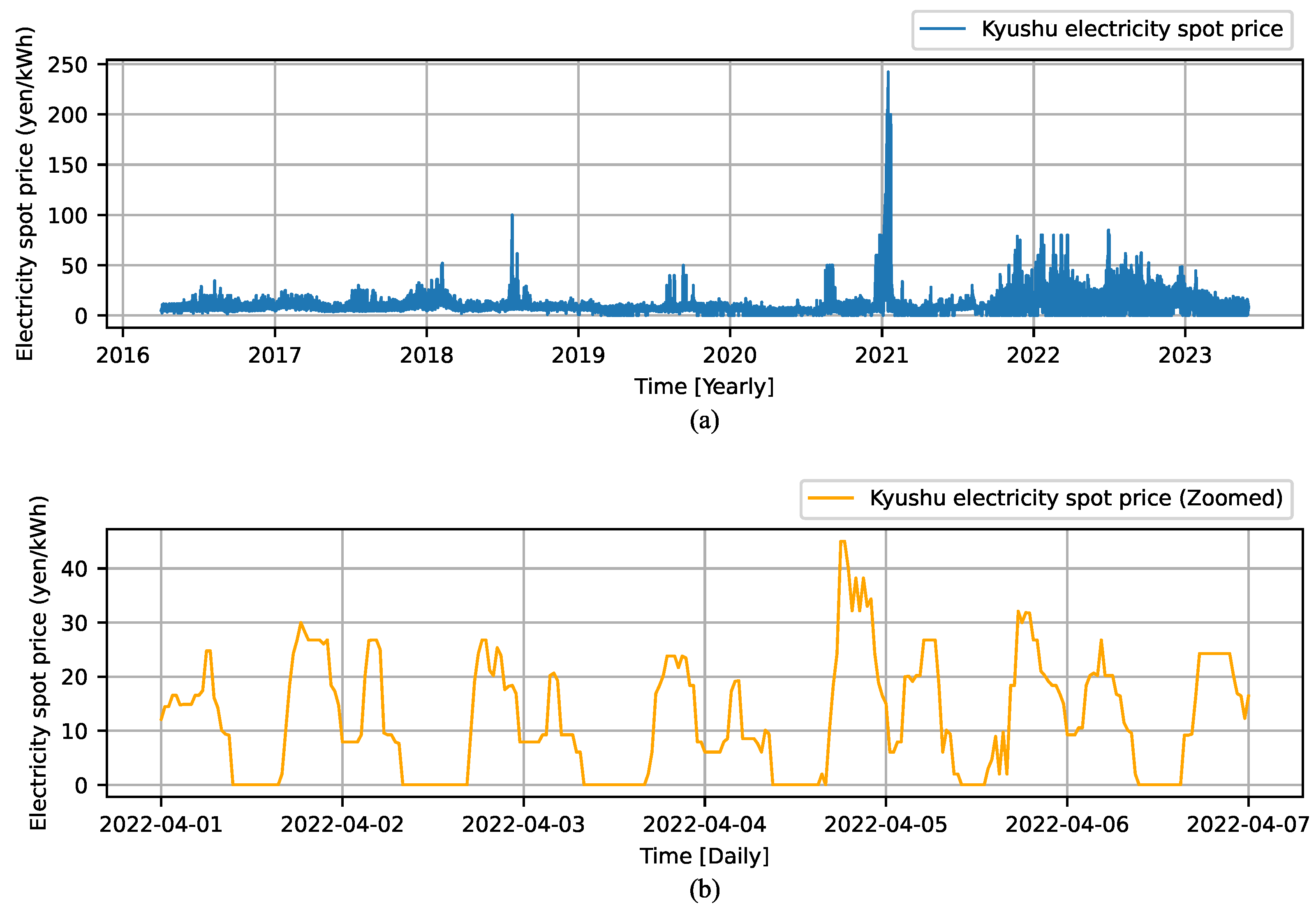
In recent years, the increased penetration of RES, particularly from wind and solar sources, has introduced an unprecedented phenomenon in the US and EU electricity markets: negative day-ahead electricity price [27]. This development can be attributed primarily to two interconnected factors. First, the inherent intermittency and unpredictability of RES can occasionally lead to generation surpassing demand, leading to an oversupply. Second, conventional power plants, including nuclear and coal, often find it challenging to ramp down production swiftly or cost-effectively. During periods of high renewable energy output, these plants may opt to maintain operations, effectively paying consumers to use the excess electricity rather than incurring the costs associated with shutting down and restarting. The occurrence of negative electricity prices has become increasingly frequent. For instance, during the final two weeks of 2012, day-ahead electricity prices in Germany turned negative on three occasions, an event that was considered unusual at the time, as emphasized by Shiri et al. [28]. Recent findings by Seel et al. [27] indicate that, in 2020, solar and wind energy were principal contributors to negative prices in both the US and EU electricity markets. Such negative prices, while posing challenges, highlight the imperative for proficient grid management, adaptable demand–response systems, and energy storage solutions to keep pace with the escalating contribution of RES [29,30]. However, the situation in Japan presents a distinct narrative. With the significant introduction of solar and wind energy into the Japanese power grid, the electricity wholesale day-ahead markets have witnessed prices approaching nearly zero JPY/kWh, specifically at 0.01 JPY/kWh (referred to as zero prices in the following sections of this paper). Notably, negative prices have been absent, a consequence of the Japanese governmental policies and regulations. The day-ahead electricity price in the Kyushu area is depicted in Figure 1a. A closer look at the intermittent zero prices is presented in Figure 1b. As evident from Figure 1a, the emergence of considerable zero prices became prominent from the year 2020 onward, largely attributable to the rapid integration of RES.
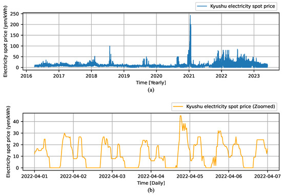
Figure 1.
Kyushu areal day-ahead electricity price [JPY/kWh] (a) and zooming-in on zero-inflated prices (b).
1.4. Paper Contributions and Organization
The contributions of this paper are summarized as follows. To address the challenges previously mentioned, this research investigates multimodal data as novel features to enhance DAEPF in Kyushu area, Japan, and compare the performance between the standalone LSTM model and the CNN–LSTM model in terms of both prediction accuracy and computation time, by utilizing a novel ensemble learning approach to address their inherent uncertainties. Moreover, to address the “zero-inflated” problem in the Japan Electric Power Exchange (JEPX) day-ahead electricity market, a novel “policy-versus-policy” strategy is employed to forecast the zero prices to half the computation time, which a traditional two-stage method requires. Furthermore, a natural logarithm transformation is utilized to improve the Skewness and Kurtosis of the electricity price to enhance the prediction accuracy. Moreover, a novel method for extracting meteorological forecast data by utilizing Google Maps is introduced. To the best of the authors’ knowledge, no prior work has combined these specific features together for accurate DAEPF.
The remainder of this paper is organized as follows. Section 2 details the methodology adopted in this study and presents the comprehensive structure of the LSTM and CNN–LSTM models used for DAEPF. Section 3 describes the data architecture underpinning the DAEPF models. Section 4 reports the performance metrics of the DAEPF results and validates the efficacy of the proposed feature sets. Finally, Section 5 concludes the paper and discusses potential directions for future research.
2. Methodology
2.1. LSTM and CNN–LSTM Forecasting Models
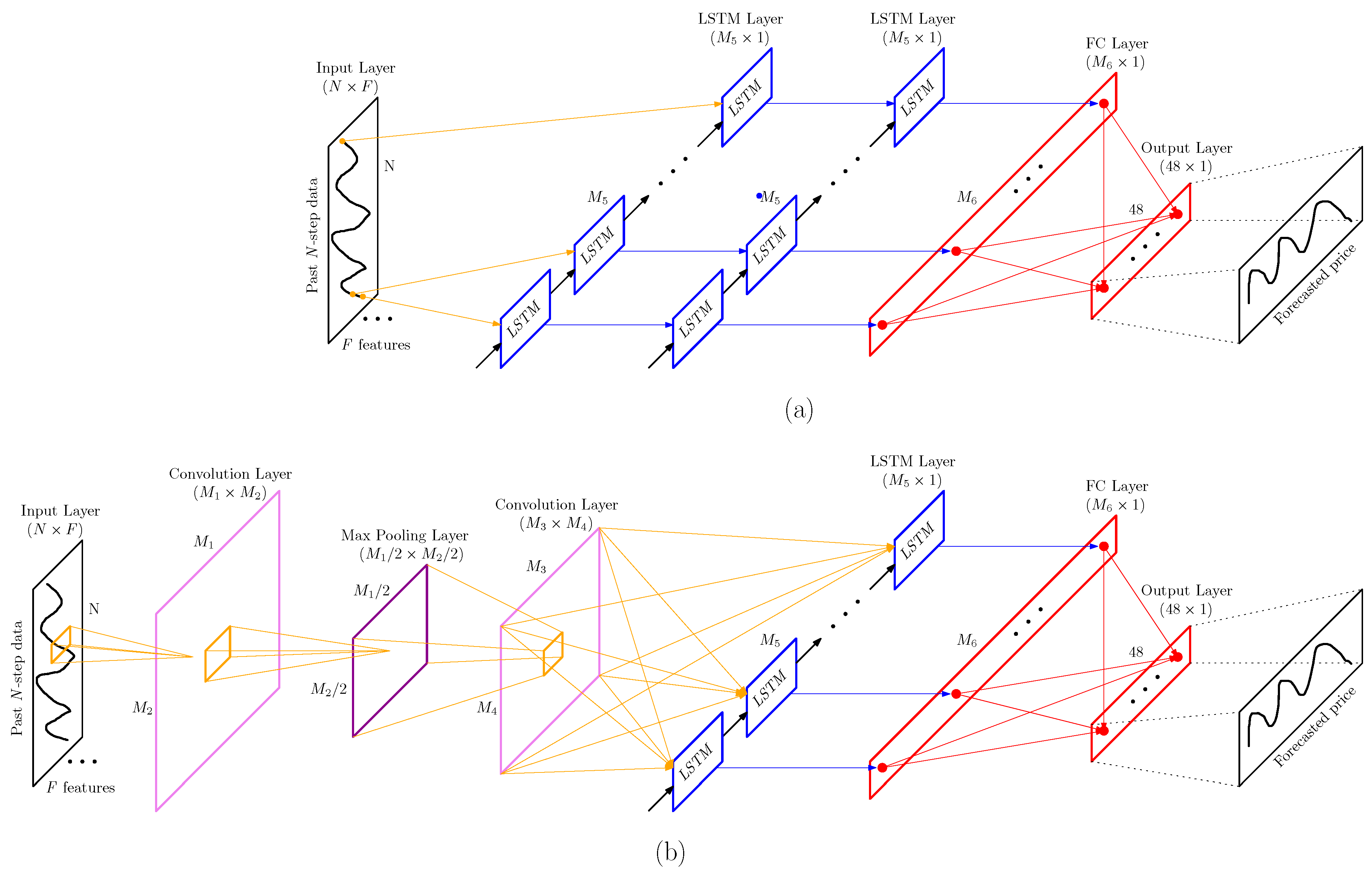
An LSTM model and a CNN–LSTM model were designed and employed for DAEPF and for comparison using the Python Tensorflow Keras library, given their demonstrated performance in time series forecasting, as discussed in Section 1.2. The architectures of the LSTM and CNN–LSTM models are delineated in Figure 2, and the hyperparameters were selected empirically based on optimal performance. The LSTM model comprises two LSTM layers with the same number of units, followed by a fully-connected (FC) Layer. The initiation of the CNN–LSTM model begins with an input layer that accommodates the input data. Following this, the data traverses through a one-dimensional convolution layer, employing the Rectified Linear Unit (ReLU) activation function. Subsequently, a max pooling layer is applied to the convolutional output, assisting in reducing the spatial dimensions of the output feature maps. Another convolution layer follows, facilitating further feature extraction from the data. The ensuing layer is an LSTM Layer, with the same number of units as the LSTM layers in the LSTM model, adept at capturing the temporal dependencies in the time-series data. The output of the LSTM Layer is then routed through an FC layer, producing the final output of the model. The LSTM and CNN–LSTM models are compiled using the Adam optimizer with a learning rate of 0.001, with the mean absolute error (MAE) chosen as both the loss function and the metric. To prevent overfitting, the batch size and number of training epochs for both models were set to 2048 and 50, respectively, for each training iteration. Subsequently, the performance of the LSTM and CNN–LSTM models are then compared.
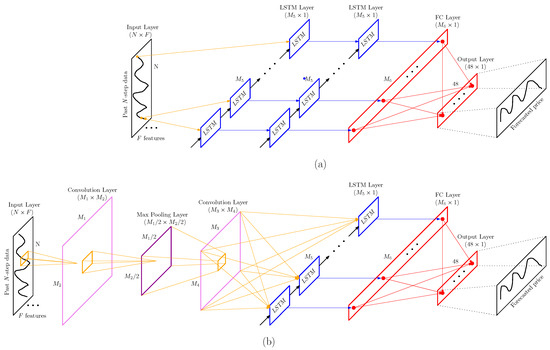
Figure 2.
Schematic of the architectures of the (a) LSTM and (b) CNN–LSTM models.
2.2. Ensemble Learning Strategy
Given the inherent variability of neural network models, which stems from their sensitivity to initial conditions and the stochastic nature of their training, training the same neural network multiple times and averaging the predictions can mitigate individual model errors. This leads to enhanced prediction performance, as different models will not make the same errors on the identical test set [31,32]. Based on this understanding, a novel ensemble learning approach was implemented. The LSTM and CNN–LSTM models underwent multiple training iterations for each feature set defined in Section 3.4. Subsequently, all individual predictions were aggregated using a simple averaging method to construct the final ensemble prediction. The ensemble learning process is described in Equation (1), where N represents the total number of predictions, and k denotes the index of each individual prediction. In accordance with the central limit theorem, which posits that the distribution of the average of a large number of independent, identically distributed variables will approximate normality, this study selected as the number of training iterations for ensemble predictions.
For clarity, the pseudo-code for the ensemble learning procedure is outlined in Algorithm 1.
| Algorithm 1 Ensemble Learning Procedure |
|
2.3. “Policy-Versus-Policy” Zero Prices Forecasting Strategy
As is shown in Figure 1b, the considerable durations of zero prices in the target variable create a zero-inflated regression problem in machine learning after data normalization. However, it is almost impossible for most machine learning models, including Random Forest (RF), Support Vector Regression (SVR), and neural networks, to continuously output zeros. The traditional method to solve the zero-inflated regression problem typically applies a two-stage approach: one binary classification model to identify the zeros and another regression model to predict the non-zero values, which doubles the computation time and training cost. In this study, we introduce a novel method to address this issue. The solution begins with an understanding of broader trends in global day-ahead electricity markets. As highlighted by Seel et al. [27], the abundance of RES can lead to negative day-ahead electricity prices in the US and EU. Drawing from this, we infer that negative pricing is a natural consequence of RES abundance. In Japan, the current policy dictates that day-ahead electricity prices cannot drop below 0.01 JPY/kWh, thereby preventing them from turning negative. Assuming that the circumstances leading to negative prices in the US and EU are similar to those in Japan, it is reasonable to infer that the explanatory variables in both scenarios would exhibit similar patterns. Feeding these Japanese explanatory variables into a machine learning regression model would naturally produce negative prices, as the model is not constrained by Japan’s minimum pricing policy. Hence, by leveraging this premise, zero prices can be forecast by translating any negative outputs from the model to zeros. This novel approach effectively functions as a policy-versus-policy forecasting strategy, reflecting real-world conditions. Equation (2) illustrates the zero price calculation procedure.
2.4. Performance Evaluation
3. Data Preparation
This study utilizes multimodal data to enhance DAEPF, comprising the areal day-ahead electricity price (Kyushu), day-ahead system electricity price, rolling features of areal day-ahead electricity price, areal actual power generation (Kyushu), areal meteorological forecast data (Kyushu), and calendar forecast data. In this study, since photovoltaic (PV) power is the primary RES in the Kyushu area due to its substantially greater installed capacity compared to wind power, features pertaining to wind power are not incorporated into the current investigation.
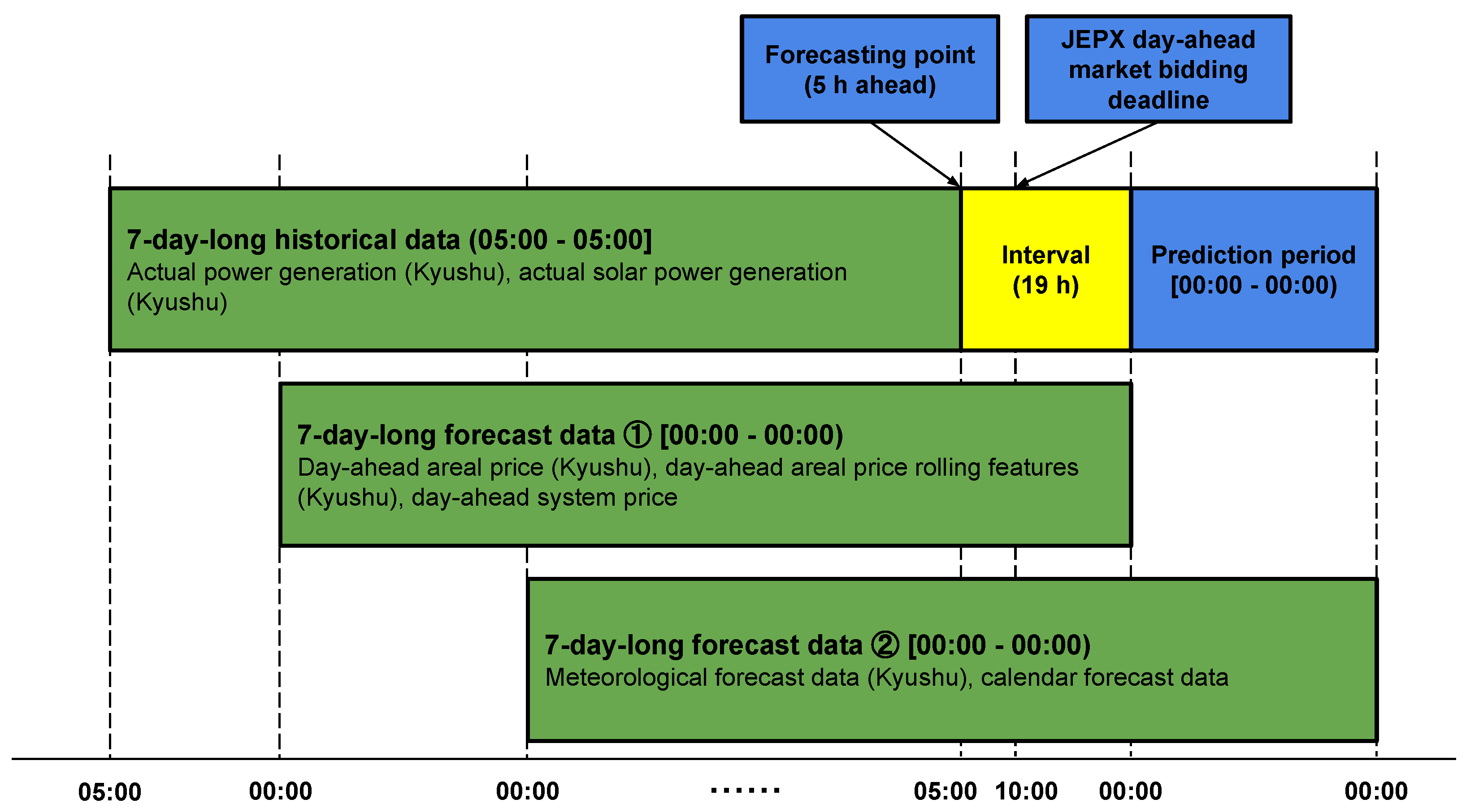
The overall data architecture and the corresponding time frame are illustrated in Figure 3. The input data are segmented by their temporal delay into three green blocks. To maintain consistency with the JEPX day-ahead electricity price data, all input data were linearly interpolated to a time resolution of 30 min. A 7-day moving window was applied to the input data before being fed into the DAEPF models. In the JEPX day-ahead electricity market, all transactions must be finalized by the bidding deadline of 10:00 JST. Given the computational requirements and the complexities of the forecasting process, a 5 h buffer before the deadline has been established. The explanatory variables include data up to 05:00 JST on the day before the forecast day. The forecasting period covers the entire following day, from 00:00 JST to 23:30 JST, encompassing a total of 48 time frames.
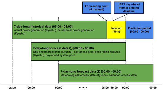
Figure 3.
Illustration of the data architecture of the explanatory variables, highlighting the time delays among different data.
Regarding the outliers issue, extreme values in day-ahead electricity prices and power generation data are considered significant and not anomalies. For meteorological forecast data, since individual forecast points have forecasting errors, the outliers are mitigated by averaging the data over the Kyushu area. This approach reduces the impact of individual errors and ensures stable input for the DAEPF model.
3.1. Electricity Data
3.1.1. Day-Ahead Electricity Price
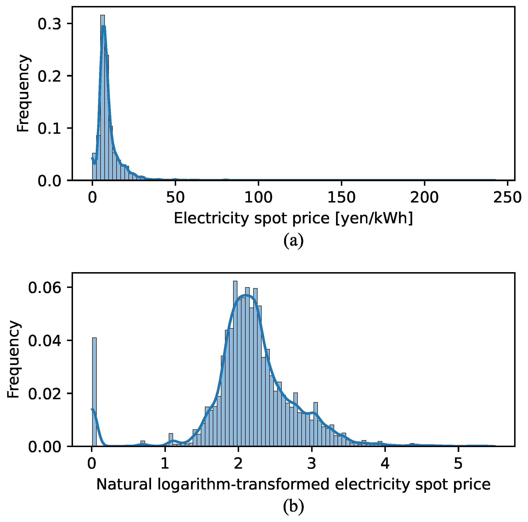
The day-ahead electricity prices (JPY/kWh) at a 30 min resolution, encompassing both the areal day-ahead electricity price and the day-ahead system electricity price, were obtained from the JEPX official website [33]. The distribution of the Kyushu areal day-ahead electricity price, as illustrated in Figure 4a, exhibits pronounced Skewness and Kurtosis, indicating a skewed distribution. Neural network models typically assume that input data are normally distributed or at least exhibit symmetry, as this facilitates the model’s learning process by providing a standardized scale for the input features. Deviations from normality, such as Skewness and Kurtosis, can introduce biases in the model’s predictions and affect the efficiency of the learning algorithm. To mitigate these effects, a natural logarithm transformation was applied to the day-ahead Kyushu areal electricity price, as detailed in Equation (6). This transformation, a common technique in statistical normalization, reduces the impact of Skewness and Kurtosis by compressing the scale of the distribution, thereby enhancing symmetry and reducing the influence of outliers. The effectiveness of the natural logarithm transformation is quantitatively evidenced by the reduction in Skewness and Kurtosis of the price data, as shown in Table 1 and Figure 4b. Following the model’s prediction output, an exponential back-transformation, defined in Equation (7), is applied to convert the forecast values back to their original scale.
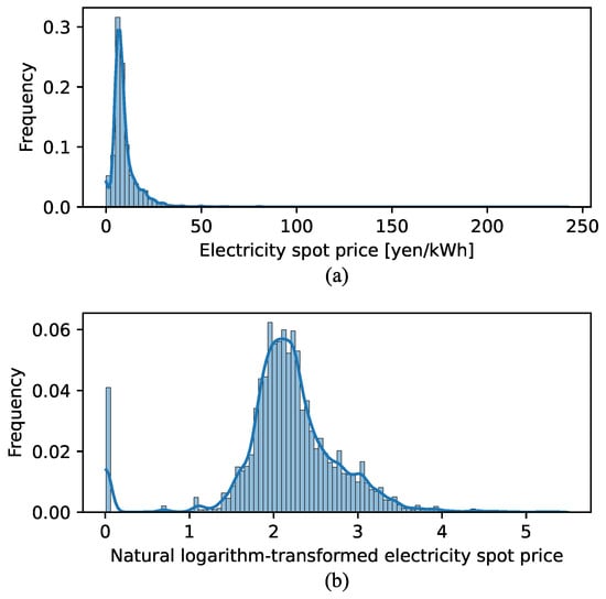
Figure 4.
Distribution of Kyushu areal day-ahead electricity price (a) and the corresponding distribution after the natural logarithm transformation (b).

Table 1.
Skewness and Kurtosis of the original and natural logarithm-transformed Kyushu areal day-ahead electricity prices during 5 April 2016 to 31 December 2021.
Feature engineering was conducted to the day-ahead Kyushu areal electricity price using a method that involves calculating rolling statistics (minimum, maximum, mean, and standard deviation) with a rolling window. This method is crucial for capturing temporal patterns and trends, which are essential for time series feature extraction. The equations for these calculations are provided in Equations (8)–(11), where t indicates the current time step, and w indicates the length of the rolling window. The length of the rolling window was chosen to be 3 days, i.e., w = 144.
3.1.2. Actual Power Generation
The actual power generation data (MW) at a 5-min resolution in the Kyushu area were obtained from the Organization for Cross-regional Coordination of Transmission Operators, Japan (OCCTO) [34], including the actual total power generation and actual solar power generation.
3.2. Meteorological Forecast Data
The meteorological forecast data at a 1-h resolution were obtained from the Japan Meteorological Business Support Center (JMBSC) [35]. The Mesoscale Model Grid Point Value (MSM-GPV) consists of ten categories of meteorological data: the U-Component of Wind (UGRD), representing wind speed in the east–west direction with positive values indicating westerly winds; the V-Component of Wind (VGRD), representing wind speed in the north–south direction with positive values indicating southerly winds; temperature (TMP); relative humidity (RH); Low Cloud Cover (LCDC), indicating low-level cloudiness; Middle Cloud Cover (MCDC), indicating mid-level cloudiness; High Cloud Cover (HCDC), indicating high-level cloudiness; Total Cloud Cover (TCDC); Accumulated Precipitation (APCP); and Downward Shortwave Radiation Flux (DSWRF), indicative of solar radiation reaching the Earth’s surface.
The JMBSC issues meteorological forecasts six times daily at 03:00, 06:00, 09:00, 15:00, 18:00, and 21:00 UTC, providing high-resolution, hourly updates at the surface level. These forecasts cover a geographic area from 22.4° N, 120° E to 47.6° N, 150° E, encompassing the whole area of Japan, and are disseminated on an equal latitude–longitude grid with a resolution of 0.05° × 0.0625° (505 by 481 grid points). The data are distributed in the GRIB2 format, with each 39 h forecast file approximately 293 MB in size, resulting in about 1758 MB of data per 1 day. According to the forecasting time point of 05:00 JST, data up to 18:00 UTC were utilized.
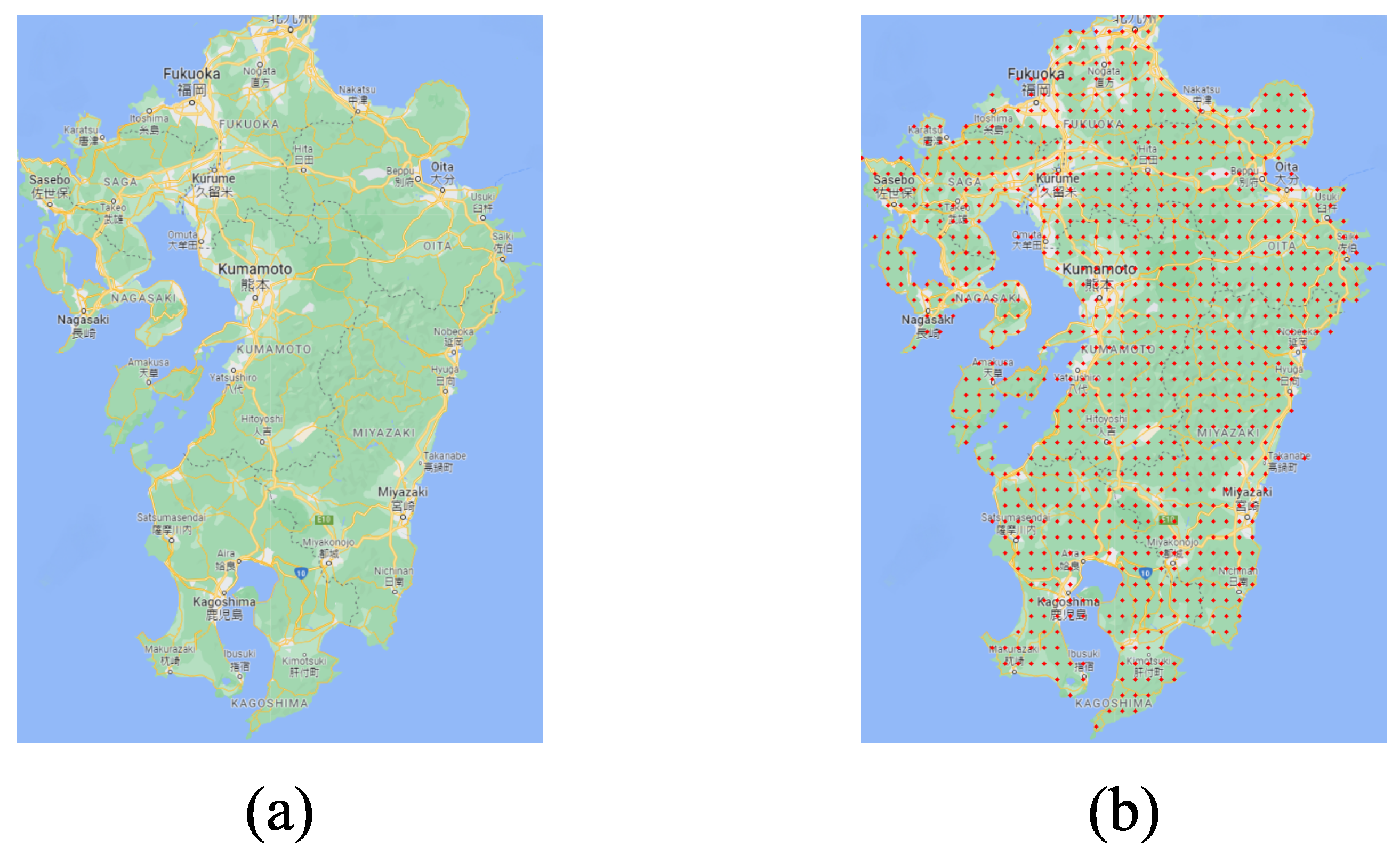
The Kyushu area map was a rectangular screenshot from the Google Maps Styling Wizard [36]. The identification of the land areas from the Kyushu area map was conducted using the Python OpenCV library [37]. Figure 5a displays the original screenshot of the Kyushu area map. In this step, pixels that are not within the defined blue color range, specifically lower-bound HSV values of [100, 50, 50] and upper-bound values of [130, 255, 255], are identified as land. Subsequently, Figure 5b showcases the delineated land areas from Figure 5a, with red dots marking these regions. After the identification of land areas, the meteorological data of all the land area pixels were averaged as input features.
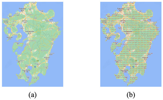
Figure 5.
Kyushu area map (a) and the identified land areas (b). Map data: ©2024 Google, TMap Mobility.
The reason for utilizing the aforementioned meteorological data is as follows. According to the American Society of Heating, Refrigerating and Air-Conditioning Engineers (ASHRAE) [38], an occupant’s thermal comfort is influenced by air temperature and relative humidity (RH). The utility of air temperature and RH in modeling thermal comfort has been substantiated in previous studies [39,40]. Solar radiation significantly impacts the output of photovoltaic (PV) panels, thereby necessitating the inclusion of Downward Shortwave Radiation Flux (DSWRF) data. Additionally, cloud cover at different levels, represented by Low Cloud Cover (LCDC), Middle Cloud Cover (MCDC), High Cloud Cover (HCDC), and Total Cloud Cover (TCDC), also affects solar radiation. Hence, these factors were included in the analysis. The U-Component (UGRD) and V-Component (VGRD) of Wind are relevant for modeling wind power generation, which is why they were considered. Lastly, Accumulated Precipitation (APCP) influences the generation of hydropower and small-scale hydro power, making it a pertinent variable for inclusion.
3.3. Calendar Forecast Data
The calendar forecast data which integrate the cyclic features and Japanese holidays, aimed to enhance the DAEPF accuracy by accounting for the unique electricity consumption behaviors associated with specific time periods, were used as features.
3.3.1. Cyclic Features
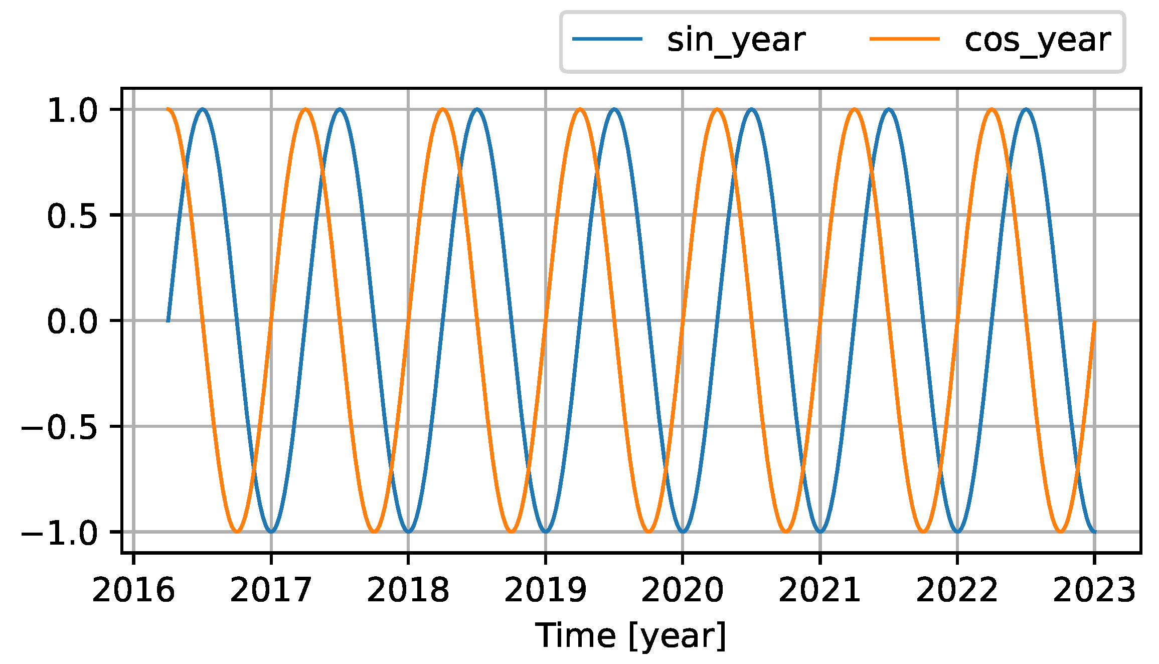
When modeling time series data, capturing the inherent cyclicity of time-related features is essential. Many features, such as hours of the day, days of the week, or months of the year, exhibit periodic behavior. For instance, the pattern of human activity at 06:00 JST is more similar to 06:00 JST of the next day. Traditional linear representations of time fail to capture this cyclical relationship. One effective method to account for this cyclicity is to transform time-related features using trigonometric functions, specifically sine and cosine transformations. By representing features like days, weeks, months, and years as points on a unit circle using sine and cosine values, we can maintain the closeness of cyclical times as adjacent. In this study, we employ sine and cosine transformations with periods corresponding to common cyclical patterns: 1 day, 1 week, 1 month, and 1 year. For instance, the sine and cosine waves with a period of 1 year is shown in Figure 6. Such transformations have been acknowledged in foundational time series literature as a robust method to encapsulate periodic patterns in data [41,42,43,44,45].
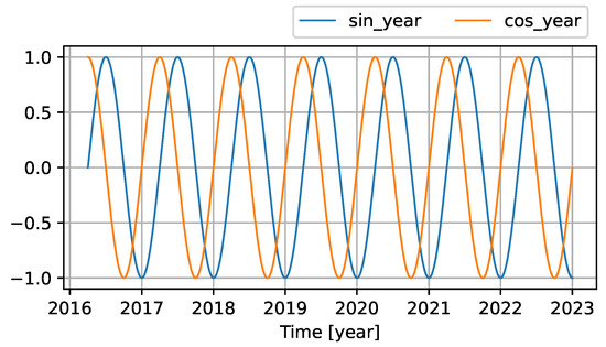
Figure 6.
Sine and cosine waves with a period of 1 year.
3.3.2. Holiday Features
Japanese holidays and non-holidays were encoded into numerical labels, with holidays labeled as 1 and non-holidays as 0. These holidays include national holidays, Golden Week from 29 April–5 May, and the New Year’s period from 29 December–3 January.
3.4. Multiple Feature Sets
To analyze and compare the validity of the proposed features, a strategy is proposed that involves removing each feature set one at a time from all proposed features and using the remaining features to evaluate and compare prediction accuracy, as shown in Table 2.
Table 2.
Performance metrics of the CNN–LSTM and LSTM ensemble learning models using different combinations of the proposed features during the test period (1 January 2022–31 December 2022). The highest prediction accuracies are highlighted in bold.
3.5. Prediction Methods
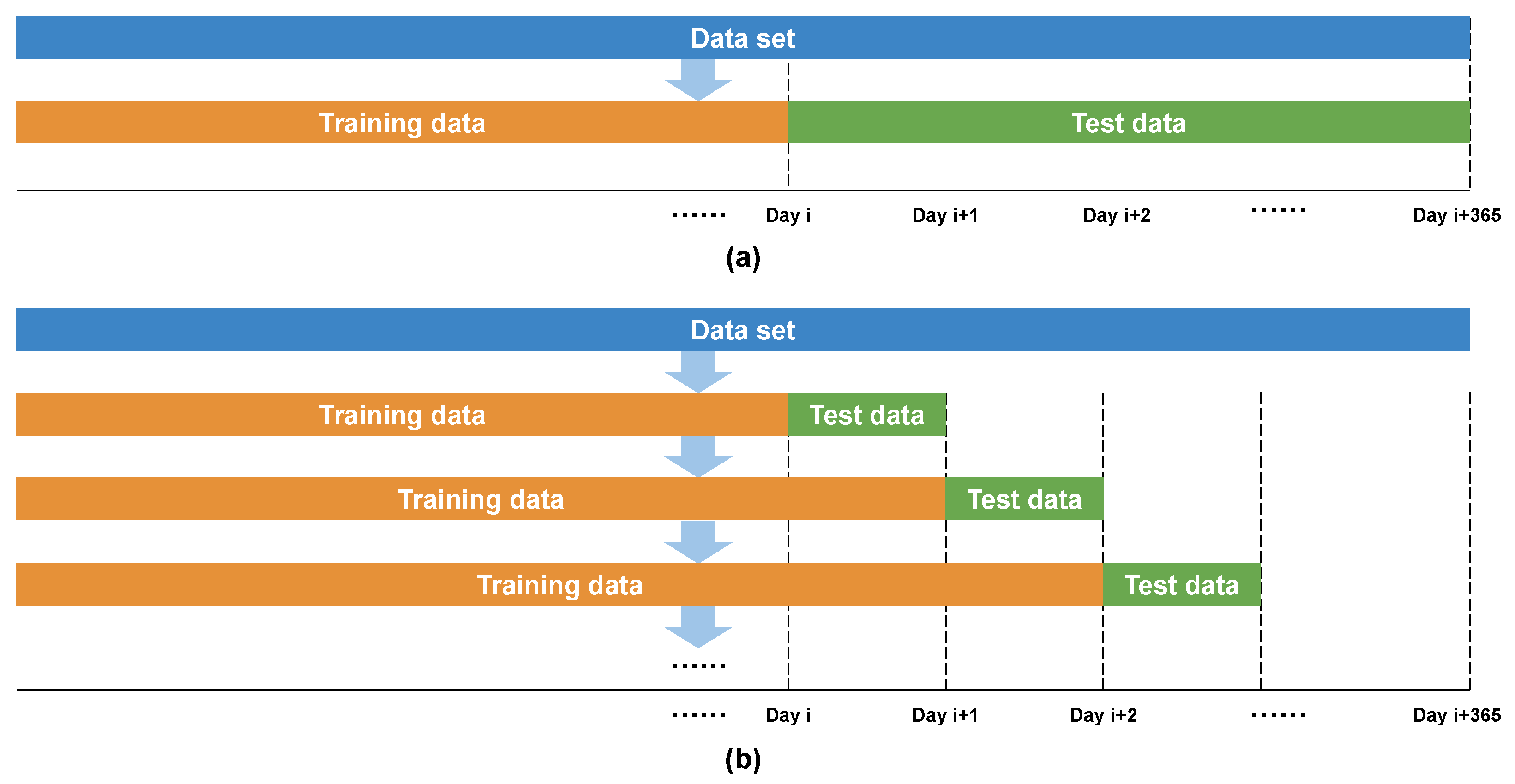
Two prediction methods were utilized, as illustrated in Figure 7. Prediction method (a) is used to validate the performance of proposed features as it requires much less training time compared with the day-by-day prediction method (prediction method (b)) shown in Figure 7b. For validation of the proposed features, the training data span from 5 April 2016—the date marking the full liberalization of the electricity retail market—to 31 December 2021. The testing period ranges from 1 January 2022 to 31 December 2022. Considering that the test data span an entire year, the probability of the results being attributable to random chance is considerably minimized.

Figure 7.
Schematics of the one-time prediction method (a) and the day-by-day prediction method (b).
After selecting the features with the best prediction performance, the day-by-day prediction method was conducted to explore the actual prediction accuracy in real-world application scenarios using these optimal features. Specifically, the test range is the next whole day for each training data range, and the training data are updated for every predicted next whole day. For the day-by-day prediction method, the testing period ranges from 1 March 2023 to 31 March 2023, and the training data span from 5 April 2016 to the day before the predicted day. For comparison during the same testing period, the prediction method (a) was also used, as shown in Table 3.
Table 3.
Performance metrics of prediction methods (a) and (b) using the CNN–LSTM ensemble learning model using all proposed features. The highest prediction accuracies are highlighted in bold.
3.6. Model Training Platform
The models were trained using two NVIDIA Quadro RTX 8000 GPUs on a Windows OS.
4. Results and Discussion
4.1. Ensemble Learning Prediction Results
Table 2 presents the performance metrics for the prediction outcomes by adjusting models, features, pre-processing (natural logarithm transformation), and ensemble learning iteration times. By observing Table 2, significant results can be summarized as follows.
- Using all features, the ensemble learning prediction with the CNN–LSTM model achieved the highest performance metrics, underscoring the efficacy and validity of the proposed features in enhancing DAEPF accuracy.
- Applying the natural logarithm transformation to the target day-ahead electricity price significantly improved performance.
- The CNN–LSTM model (30 iterations ensemble) outperformed the LSTM model (15 iterations ensemble, special case for comparison), requiring less than the training time of the LSTM model.
- Using the same ensemble learning of 30 iterations, the CNN–LSTM model outperformed the LSTM model in terms of and RMSE, though slightly weaker in MAE, requiring less than half of the training time of the LSTM model.
Table 4 shows performance metrics of individual predictions using the optimal feature set (All features) from Table 2, LSTM and CNN–LSTM models, natural logarithm transformation pre-processing, and prediction method (a). It is noteworthy in Table 4 that each training iteration results in a unique individual prediction on the test set, underscoring the inherent uncertainty in the neural network training process. Table 2 and Table 4 demonstrate that the performance metrics of ensemble predictions significantly outperform the simple average of the performance metrics from individual predictions, as well as the best individual prediction, highlighting the efficacy of the ensemble learning strategy. In addition, the average individual prediction performance of the CNN–LSTM model outperformed that of the LSTM model. Furthermore, it is evident from Table 4 that a certain individual CNN–LSTM prediction can underperform a certain individual LSTM prediction, indicating that comparing individual predictions between CNN–LSTM and LSTM models is not reliable, thereby highlighting the necessity of the ensemble learning approach.
Table 4.
Performance metrics of individual predictions using the CNN–LSTM and LSTM models with all proposed features and natural logarithm transformation pre-processing employing prediction method (a).
4.2. Day-by-Day Prediction Result
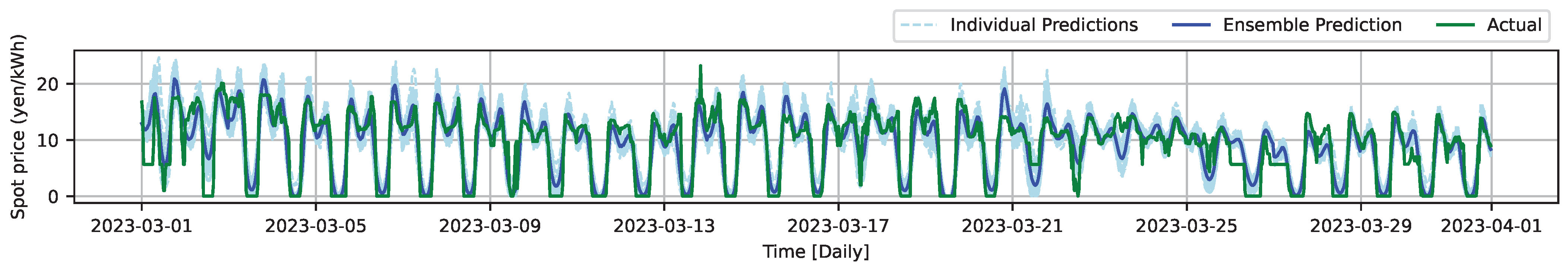
The day-by-day prediction results are shown in Figure 8. The ensemble learning metrics for prediction methods (a) and (b) are presented in Table 3. As is shown in Table 3, using the day-by-day prediction method, where the training data are incremented daily to include the most recent information, significantly enhanced performance compared with the prediction method (a), as the model consistently integrates the latest data up to the day before the prediction.
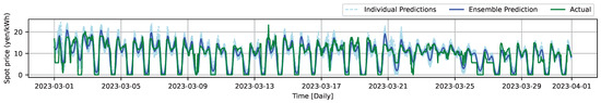
Figure 8.
Individual and ensemble predictions for the test range from 1 March 2023 to 31 March 2023, using the CNN–LSTM model and all proposed features with the natural logarithm transformation pre-processing and the day-by-day prediction method.
As can be observed from Figure 8, ensemble learning effectively reduces the variability inherent in individual model predictions. Although some individual predictions may diverge markedly from the actual values, the ensemble method, described in Equation (1), averages these forecasts to produce a more reliable final prediction. This technique aligns with the principle outlined by GoodFellow et al. [31]: averaging models is beneficial because distinct models are unlikely to repeat the same errors on the test set. On the other hand, as shown in Figure 8, the model is capable of predicting zero prices to some extent, indicating the validity of the “policy-versus-policy” zero prices forecasting strategy. Though not all instances of zero prices were successfully captured.
5. Conclusions and Future Work
DAEPF is pivotal for stakeholders in the energy market. This study has proposed an innovative DAEPF framework utilizing a CNN–LSTM ensemble learning model, incorporating areal day-ahead electricity price, day-ahead system electricity price, areal actual power generation, areal meteorological forecasts, calendar forecasts, alongside the rolling features of areal day-ahead electricity price, as explanatory variables to enhance DAEPF accuracy in the Kyushu area of Japan. The effectiveness of these multimodal features has been validated by comparing the prediction accuracy of different combinations of the proposed features.
Given that individual predictions vary significantly, it is unwise to ignore the uncertainty characteristics of neural networks in DAEPF or the feature selection process, and it is unreliable to compare single individual predictions between CNN–LSTM and LSTM models. However, by employing an ensemble learning approach, the uncertainty can be minimized and the prediction accuracy can be significantly increased. In the ensemble learning, the CNN–LSTM model outperforms the LSTM model in both prediction accuracy and computation time. The average individual prediction performance of the CNN–LSTM model surpasses that of the LSTM model.
Applying the natural logarithm transformation to the electricity price to improve the Skewness and Kurtosis has proven crucial for DAEPF prediction accuracy. The novel “policy-to-policy” strategy has been proposed and verified for zero prices forecasting, halving the computation time compared with the traditional two-stage method. Utilizing all features, the ensemble learning method achieved the highest performance metrics during the test range from 1 January 2022 to 31 December 2022.
Moving forward, by using the day-by-day prediction approach, the CNN–LSTM model achieved performance metrics of , MAE, and RMSE of 0.787, 1.936 JPY/kWh, 2.630 JPY/kWh, respectively, during the test range from 1 March 2023 to 31 March 2023. Moreover, while this study averaged meteorological data across the land areas, future work could leverage the entire spectrum of meteorological data to preserve more comprehensive information, potentially leading to even higher precision in DAEPF. In this study, ensemble learning of 30 iterations were conducted with the CNN–LSTM model. In future work, the balance between ensemble learning iteration times, computation time, increased prediction accuracy, and potential profits from the predictions should also be considered.
Author Contributions
Conceptualization, Z.W. and R.M.; methodology, Z.W.; software, Z.W.; validation, Z.W. and M.M.; formal analysis, Z.W., M.M., T.Y., M.A. and T.N.; investigation, Z.W., M.M., T.Y., M.A., T.N. and R.M.; resources, T.Y., M.A., T.N. and R.M.; data curation, Z.W., T.Y., M.A. and T.N.; writing—original draft preparation, Z.W.; writing—review and editing, Z.W. and M.M.; visualization, Z.W.; supervision, R.M.; project administration, R.M.; funding acquisition, R.M. All authors have read and agreed to the published version of the manuscript.
Funding
This research was funded by KYOCERA Corporation.
Data Availability Statement
All data generated or analyzed during this study are included in this article.
Conflicts of Interest
Authors Takeshi Yamane, Masato Ajisaka, Tatsuya Nakata were employed by the company Department of Energy Systems Research and Development, KYOCERA Corporation. The remaining authors declare that the research was conducted in the absence of any commercial or financial relationships that could be construed as a potential conflict of interest.
Abbreviations
| DAEPF | Day-ahead electricity price forecasting |
| RES | Renewable energy sources |
| OCCTO | Organization for Cross-regional Coordination of Transmission Operators, Japan |
| JMBSC | Japan Meteorological Business Support Center |
| JEPX | Japan Electric Power Exchange |
| ASHRAE | American Society of Heating, Refrigerating and Air-conditioning Engineers |
| PV | Photovoltaic |
| ARMA | Autoregressive Moving Average |
| ARIMA | Autoregressive Integrated Moving Average |
| RF | Random Forest |
| SVR | Support Vector Regression |
| MLP | Multilayer Perceptron |
| CNN | Convolutional Neural Network |
| LSTM | Long Short-Term Memory |
| CNN–LSTM | Convolutional Neural Network6-Long Short-Term Memory |
| FC | Fully-connected |
| ReLU | Rectified Linear Unit |
| MAE | Mean absolute error |
| RMSE | Root mean squared error |
| Coefficient of determination | |
| MSM-GPV | Mesoscale Model Grid Point Value |
| UGRD | U-Component of Wind |
| VGRD | V-Component of Wind |
| TMP | Temperature |
| RH | Relative humidity |
| LCDC | Low Cloud Cover |
| MCDC | Middle Cloud Cover |
| HCDC | High Cloud Cover |
| TCDC | Total Cloud Cover |
| APCP | Accumulated Precipitation |
| DSWRF | Downward Shortwave Radiation Flux |
| Symbols | |
| e | Natural logarithm |
| Minimum value of the day-ahead electricity price over a rolling window | |
| Maximum value of the day-ahead electricity price over a rolling window | |
| Mean value of the day-ahead electricity price over a rolling window | |
| Standard deviation of the day-ahead electricity price over a rolling window | |
| y | Target variable |
| Predicted target variable | |
| Ensemble prediction of the target variable | |
| n | Sequence length of the target variable |
| N | Total training times of the model |
| t | t-th value in a variable sequence |
| i | i-th value in a variable sequence |
| k | k-th individual prediction after k-th training of the model |
| w | Rolling window length |
References
- Abdelilah, Y.; Bahar, H.; Criswell, T.; Bojek, P.; Briens, F.; Le Feuvre, P. Renewables 2020: Analysis and Forecast to 2025; IEA: Paris, France, 2020. [Google Scholar]
- Weitemeyer, S.; Kleinhans, D.; Vogt, T.; Agert, C. Integration of Renewable Energy Sources in future power systems: The role of storage. Renew. Energy 2015, 75, 14–20. [Google Scholar] [CrossRef]
- Asiaban, S.; Kayedpour, N.; Samani, A.E.; Bozalakov, D.; De Kooning, J.D.M.; Crevecoeur, G.; Vandevelde, L. Wind and Solar Intermittency and the Associated Integration Challenges: A Comprehensive Review Including the Status in the Belgian Power System. Energies 2021, 14, 2630. [Google Scholar] [CrossRef]
- Huang, S.; Xiong, L.; Zhou, Y.; Gao, F.; Jia, Q.; Li, X.; Li, X.; Wang, Z.; Khan, M.W. Distributed Predefined-Time Control for Power System with Time Delay and Input Saturation. IEEE Trans. Power Syst. 2024, 1–14. [Google Scholar] [CrossRef]
- Özen, K.; Yıldırım, D. Application of bagging in day-ahead electricity price forecasting and factor augmentation. Energy Econ. 2021, 103, 105573. [Google Scholar] [CrossRef]
- Wang, K.; Yu, M.; Niu, D.; Liang, Y.; Peng, S.; Xu, X. Short-term electricity price forecasting based on similarity day screening, two-layer decomposition technique and Bi-LSTM neural network. Appl. Soft Comput. 2023, 136, 110018. [Google Scholar] [CrossRef]
- Li, W.; Becker, D.M. Day-ahead electricity price prediction applying hybrid models of LSTM-based deep learning methods and feature selection algorithms under consideration of market coupling. Energy 2021, 237, 121543. [Google Scholar] [CrossRef]
- Panapakidis, I.P.; Dagoumas, A.S. Day-ahead electricity price forecasting via the application of artificial neural network based models. Appl. Energy 2016, 172, 132–151. [Google Scholar] [CrossRef]
- He, K.; Xu, Y.; Zou, Y.; Tang, L. Electricity price forecasts using a Curvelet denoising based approach. Physica A Stat. Mech. Its Appl. 2015, 425, 1–9. [Google Scholar] [CrossRef]
- Yang, Z.; Ce, L.; Lian, L. Electricity price forecasting by a hybrid model, combining wavelet transform, ARMA and kernel-based extreme learning machine methods. Appl. Energy 2017, 190, 291–305. [Google Scholar] [CrossRef]
- Chaâbane, N. A hybrid ARFIMA and neural network model for electricity price prediction. Int. J. Electr. Power Energy Syst. 2014, 55, 187–194. [Google Scholar] [CrossRef]
- Conejo, A.J.; Plazas, M.A.; Espinola, R.; Molina, A.B. Day-ahead electricity price forecasting using the wavelet transform and ARIMA models. IEEE Trans. Power Syst. 2005, 20, 1035–1042. [Google Scholar] [CrossRef]
- Girish, G.P. Spot electricity price forecasting in Indian electricity market using autoregressive-GARCH models. Energy Strategy Rev. 2016, 11–12, 52–57. [Google Scholar] [CrossRef]
- Wang, B.; Wang, J. Energy futures price prediction and evaluation model with deep bidirectional gated recurrent unit neural network and RIF-based algorithm. Energy 2021, 216, 119299. [Google Scholar] [CrossRef]
- Chen, Y.; Wang, Y.; Ma, J.; Jin, Q. BRIM: An Accurate Electricity Spot Price Prediction Scheme-Based Bidirectional Recurrent Neural Network and Integrated Market. Energies 2019, 12, 2241. [Google Scholar] [CrossRef]
- Swapna, G.; Soman, K.P.; Vinayakumar, R. Automated detection of diabetes using CNN and CNN-LSTM network and heart rate signals. Procedia Comput. Sci. 2018, 132, 1253–1262. [Google Scholar] [CrossRef]
- Qiu, D.; Dong, Z.; Ruan, G.; Zhong, H.; Strbac, G.; Kang, C. Strategic retail pricing and demand bidding of retailers in electricity market: A data-driven chance-constrained programming. Adv. Appl. Energy 2022, 7, 100100. [Google Scholar] [CrossRef]
- Lu, W.; Li, J.; Li, Y.; Sun, A.; Wang, J. A CNN-LSTM-Based Model to Forecast Stock Prices. Complexity 2020, 2020. [Google Scholar] [CrossRef]
- Agga, A.; Abbou, A.; Labbadi, M.; Houm, Y.E.; Ou Ali, I.H. CNN-LSTM: An efficient hybrid deep learning architecture for predicting short-term photovoltaic power production. Electr. Power Syst. Res. 2022, 208, 107908. [Google Scholar] [CrossRef]
- Li, Y.; Garg, A.; Shevya, S.; Li, W.; Gao, L.; Lee Lam, J.S. A Hybrid Convolutional Neural Network-Long Short Term Memory for Discharge Capacity Estimation of Lithium-Ion Batteries. J. Electrochem. Energy Convers. Storage 2021, 19, 030901. [Google Scholar] [CrossRef]
- Li, T.; Hua, M.; Wu, X. A Hybrid CNN-LSTM Model for Forecasting Particulate Matter (PM2.5). IEEE Access 2020, 8, 26933–26940. [Google Scholar] [CrossRef]
- Kim, T.Y.; Cho, S.B. Predicting residential energy consumption using CNN-LSTM neural networks. Energy 2019, 182, 72–81. [Google Scholar] [CrossRef]
- Alhussein, M.; Aurangzeb, K.; Haider, S.I. Hybrid CNN-LSTM Model for Short-Term Individual Household Load Forecasting. IEEE Access 2020, 8, 180544–180557. [Google Scholar] [CrossRef]
- Cordoni, F. A comparison of modern deep neural network architectures for energy spot price forecasting. Digit. Financ. 2020, 2, 189–210. [Google Scholar] [CrossRef]
- Neupane, B.; Woon, W.L.; Aung, Z. Ensemble Prediction Model with Expert Selection for Electricity Price Forecasting. Energies 2017, 10, 77. [Google Scholar] [CrossRef]
- Chang, Z.; Zhang, Y.; Chen, W. Electricity price prediction based on hybrid model of adam optimized LSTM neural network and wavelet transform. Energy 2019, 187, 115804. [Google Scholar] [CrossRef]
- Seel, J.; Millstein, D.; Mills, A.; Bolinger, M.; Wiser, R. Plentiful electricity turns wholesale prices negative. Adv. Appl. Energy 2021, 4, 100073. [Google Scholar] [CrossRef]
- Shiri, A.; Afshar, M.; Rahimi-Kian, A.; Maham, B. Electricity price forecasting using Support Vector Machines by considering oil and natural gas price impacts. In Proceedings of the 2015 IEEE International Conference on Smart Energy Grid Engineering (SEGE), Oshawa, ON, Canada, 17–19 August 2015; pp. 1–5. [Google Scholar] [CrossRef]
- Barbour, E.; Wilson, G.; Hall, P.; Radcliffe, J. Can negative electricity prices encourage inefficient electrical energy storage devices? Int. J. Environ. Stud. 2014, 71, 862–876. [Google Scholar] [CrossRef]
- Marqusee, J.; Becker, W.; Ericson, S. Resilience and economics of microgrids with PV, battery storage, and networked diesel generators. Adv. Appl. Energy 2021, 3, 100049. [Google Scholar] [CrossRef]
- Goodfellow, I.; Bengio, Y.; Courville, A. Deep Learning; MIT Press: Cambridge, MA, USA, 2016. [Google Scholar]
- Chen, J.; Zeng, G.Q.; Zhou, W.; Du, W.; Lu, K.D. Wind speed forecasting using nonlinear-learning ensemble of deep learning time series prediction and extremal optimization. Energy Convers. Manag. 2018, 165, 681–695. [Google Scholar] [CrossRef]
- Japan Electric Power Exchange. Day Ahead Market. 2023. Available online: https://www.jepx.jp/en/electricpower/market-data/spot/ (accessed on 19 August 2023).
- Organization for Cross-Regional Coordination of Transmission Operators, Japan. Menu. 2023. Available online: https://occtonet3.occto.or.jp/public/dfw/RP11/OCCTO/SD/LOGIN_login (accessed on 1 August 2023).
- Japan Meteorological Business Support Center. Numerical Weather Prediction Model GPV-MSM. 2023. Available online: http://www.jmbsc.or.jp/jp/online/file/f-online10200.html (accessed on 15 July 2023).
- Google Maps. Available online: https://www.google.com/maps/@36.2932467,137.3408308,6z?entry=ttu (accessed on 3 May 2024).
- OpenCV Team. OpenCV Library. 2023. Available online: https://opencv.org/ (accessed on 19 August 2023).
- ANSI/ASHRAE Standard 55-2017; Thermal Environmental Conditions for Human Occupancy. ASHRAE Inc.: Peachtree Corners, GA, USA, 2017.
- Wang, Z.; Matsuhashi, R.; Onodera, H. Towards wearable thermal comfort assessment framework by analysis of heart rate variability. Build. Environ. 2022, 223, 109504. [Google Scholar] [CrossRef]
- Wang, Z.; Matsuhashi, R.; Onodera, H. Intrusive and non-intrusive early warning systems for thermal discomfort by analysis of body surface temperature. Appl. Energy 2023, 329, 120283. [Google Scholar] [CrossRef]
- Cleveland, W.S.; Devlin, S.J.; Grosse, E. Regression by local fitting: Methods, properties, and computational algorithms. J. Econ. 1988, 37, 87–114. [Google Scholar] [CrossRef]
- Korenberg, M.J. A robust orthogonal algorithm for system identification and time-series analysis. Biol. Cybern. 1989, 60, 267–276. [Google Scholar] [CrossRef] [PubMed]
- Taylor, S.J.; Letham, B. Forecasting at Scale. Am. Stat. 2018, 72, 37–45. [Google Scholar] [CrossRef]
- Hyndman, R.J.; Athanasopoulos, G. Forecasting: Principles and Practice; OTexts: Melbourne, Australia, 2018. [Google Scholar]
- Box, G.E.P.; Jenkins, G.M.; Reinsel, G.C.; Ljung, G.M. Time Series Analysis: Forecasting and Control; John Wiley & Sons: Hoboken, NJ, USA, 2015. [Google Scholar]
Disclaimer/Publisher’s Note: The statements, opinions and data contained in all publications are solely those of the individual author(s) and contributor(s) and not of MDPI and/or the editor(s). MDPI and/or the editor(s) disclaim responsibility for any injury to people or property resulting from any ideas, methods, instructions or products referred to in the content. |
© 2024 by the authors. Licensee MDPI, Basel, Switzerland. This article is an open access article distributed under the terms and conditions of the Creative Commons Attribution (CC BY) license (https://creativecommons.org/licenses/by/4.0/).