
Intelligent Learning Method for Capacity Estimation of Lithium-Ion Batteries Based on Partial Charging Curves


Abstract
1. Introduction
2. Research Methods
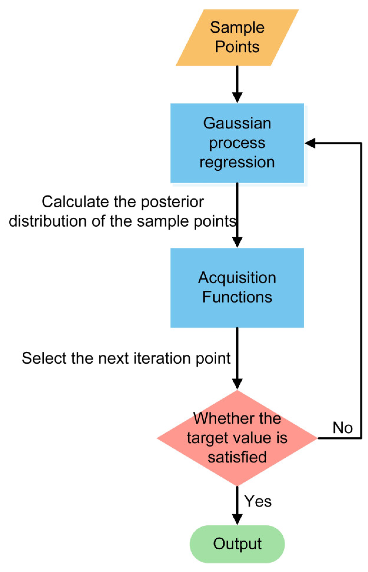
2.1. Bayesian Optimization
2.2. Neural Network Architecture and Description
2.2.1. Principle
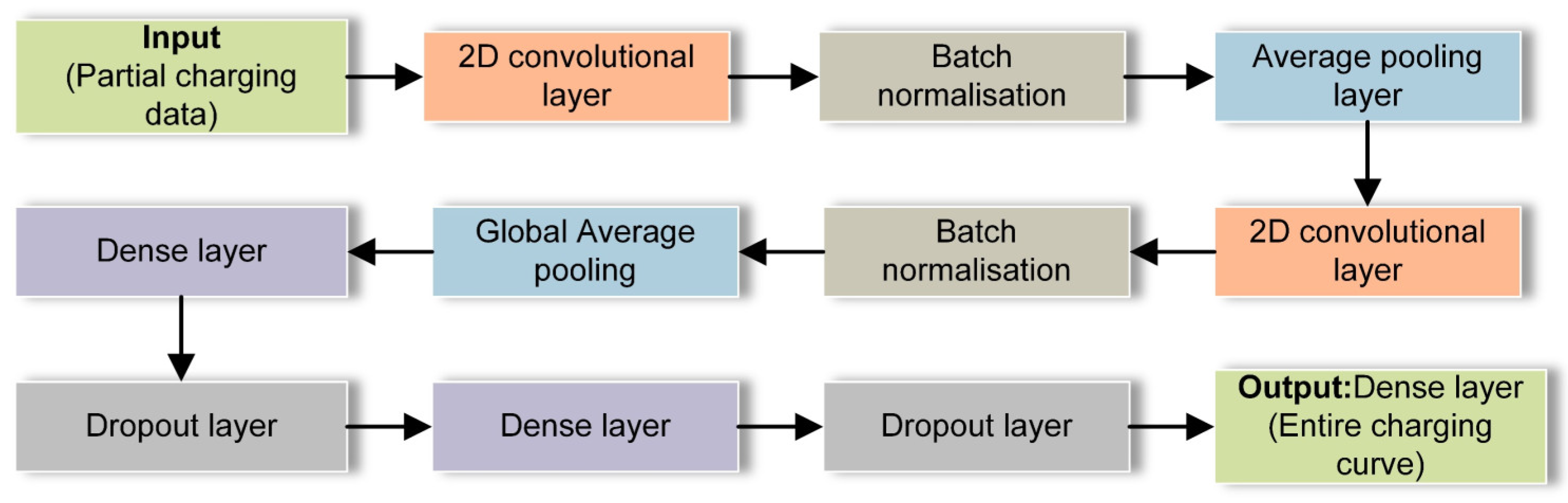
2.2.2. Architecture
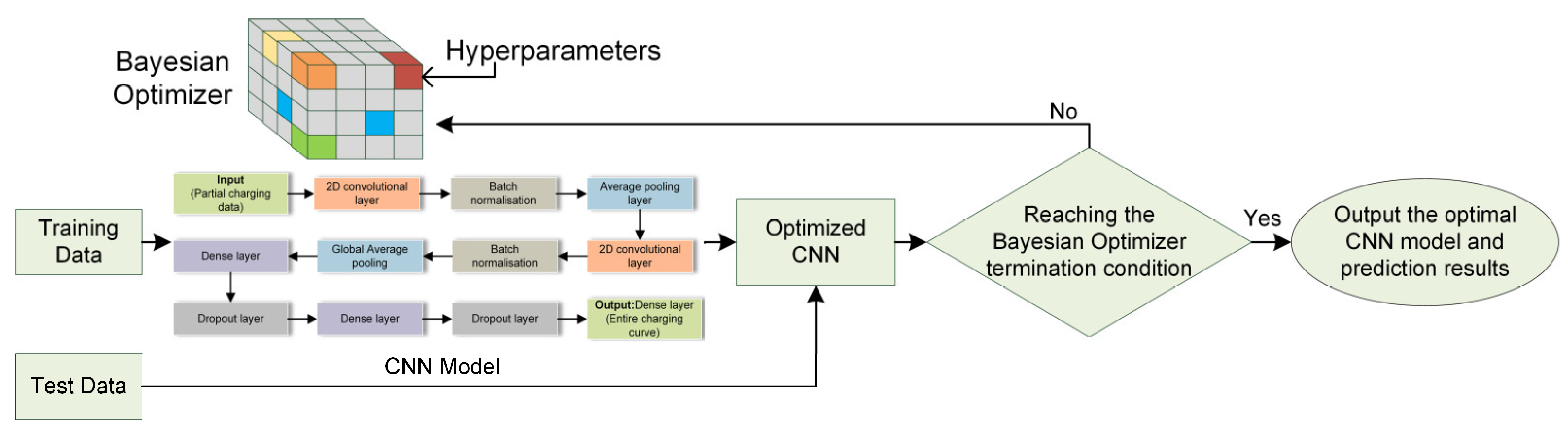
2.3. Neural Network Training under Bayesian Optimization
3. Empirical Analysis
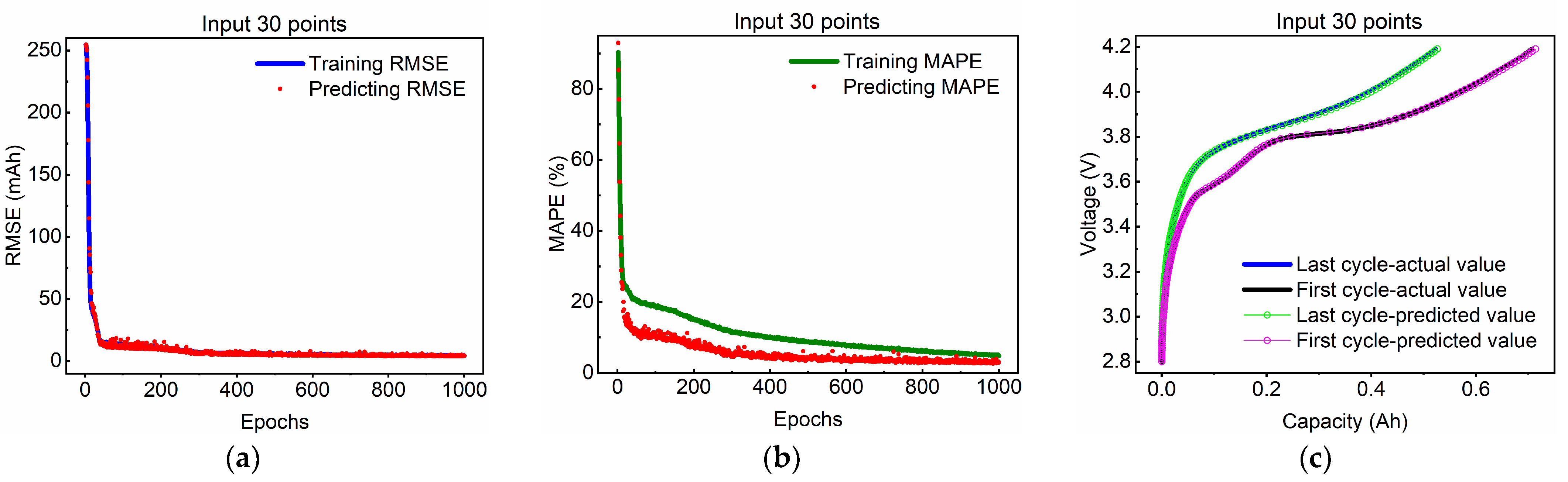
3.1. Complete Charging Curve Estimation
3.2. Different Input Data Length Validation
3.3. Comparison of Different Approaches
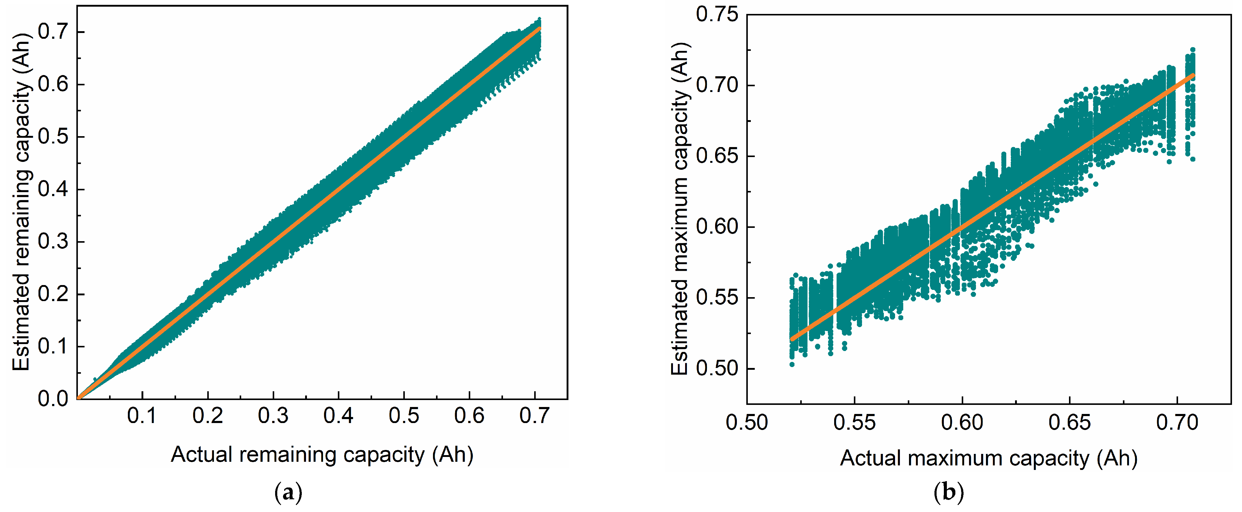
4. Maximum and Remaining Capacity Estimates
5. Conclusions
Author Contributions
Funding
Data Availability Statement
Conflicts of Interest
References
- Shen, L.; Cheng, Q.; Cheng, Y.; Wei, L.; Wang, Y. Hierarchical Control of DC Micro-Grid for Photovoltaic EV Charging Station Based on Flywheel and Battery Energy Storage System. Electr. Power Syst. Res. 2020, 179, 106079. [Google Scholar] [CrossRef]
- Wang, S.-L.; Tang, W.; Fernandez, C.; Yu, C.-M.; Zou, C.-Y.; Zhang, X.-Q. A Novel Endurance Prediction Method of Series Connected Lithium-Ion Batteries Based on the Voltage Change Rate and Iterative Calculation. J. Clean. Prod. 2019, 210, 43–54. [Google Scholar] [CrossRef]
- Wróblewski, P.; Kupiec, J.; Drożdż, W.; Lewicki, W.; Jaworski, J. The Economic Aspect of Using Different Plug-In Hybrid Driving Techniques in Urban Conditions. Energies 2021, 14, 3543. [Google Scholar] [CrossRef]
- Wróblewski, P.; Drożdż, W.; Lewicki, W.; Miązek, P. Methodology for Assessing the Impact of Aperiodic Phenomena on the Energy Balance of Propulsion Engines in Vehicle Electromobility Systems for Given Areas. Energies 2021, 14, 2314. [Google Scholar] [CrossRef]
- Lu, J.; Xiong, R.; Tian, J.; Wang, C.; Hsu, C.-W.; Tsou, N.-T.; Sun, F.; Li, J. Battery Degradation Prediction against Uncertain Future Conditions with Recurrent Neural Network Enabled Deep Learning. Energy Storage Mater. 2022, 50, 139–151. [Google Scholar] [CrossRef]
- Barai, A.; Uddin, K.; Dubarry, M.; Somerville, L.; McGordon, A.; Jennings, P.; Bloom, I. A Comparison of Methodologies for the Non-Invasive Characterisation of Commercial Li-Ion Cells. Prog. Energy Combust. Sci. 2019, 72, 1–31. [Google Scholar] [CrossRef]
- Song, L.; Zhang, K.; Liang, T.; Han, X.; Zhang, Y. Intelligent State of Health Estimation for Lithium-Ion Battery Pack Based on Big Data Analysis. J. Energy Storage 2020, 32, 101836. [Google Scholar] [CrossRef]
- Xia, B.; Zhang, Z.; Lao, Z.; Wang, W.; Sun, W.; Lai, Y.; Wang, M. Strong Tracking of a H-Infinity Filter in Lithium-Ion Battery State of Charge Estimation. Energies 2018, 11, 1481. [Google Scholar] [CrossRef]
- Hannan, M.A.; Lipu, M.S.H.; Hussain, A.; Ker, P.J.; Mahlia, T.M.I.; Mansor, M.; Ayob, A.; Saad, M.H.; Dong, Z.Y. Toward Enhanced State of Charge Estimation of Lithium-Ion Batteries Using Optimized Machine Learning Techniques. Sci. Rep. 2020, 10, 4687. [Google Scholar] [CrossRef]
- Chen, Z.; Zhao, H.; Shu, X.; Zhang, Y.; Shen, J.; Liu, Y. Synthetic State of Charge Estimation for Lithium-Ion Batteries Based on Long Short-Term Memory Network Modeling and Adaptive H-Infinity Filter. Energy 2021, 228, 120630. [Google Scholar] [CrossRef]
- Jiao, M.; Wang, D.; Qiu, J. A GRU-RNN Based Momentum Optimized Algorithm for SOC Estimation. J. Power Sources 2020, 459, 228051. [Google Scholar] [CrossRef]
- Liu, Y.; Li, J.; Zhang, G.; Hua, B.; Xiong, N. State of Charge Estimation of Lithium-Ion Batteries Based on Temporal Convolutional Network and Transfer Learning. IEEE Access 2021, 9, 34177–34187. [Google Scholar] [CrossRef]
- Yuan, H.; Liu, J.; Zhou, Y.; Pei, H. State of Charge Estimation of Lithium Battery Based on Integrated Kalman Filter Framework and Machine Learning Algorithm. Energies 2023, 16, 2155. [Google Scholar] [CrossRef]
- Gulcu, A.; Kus, Z. Hyper-Parameter Selection in Convolutional Neural Networks Using Microcanonical Optimization Algorithm. IEEE Access 2020, 8, 52528–52540. [Google Scholar] [CrossRef]
- Bergstra, J.; Bengio, Y. Random Search for Hyper-Parameter Optimization. J. Mach. Learn. Res. 2012, 13, 281–305. [Google Scholar]
- Yang, G.; Tian, X.; Li, H.; Deng, H.; Li, H. Target Recognition Using of PCNN Model Based on Grid Search Method. dtcse 2017. [CrossRef]
- Wang, J.; Xu, J.; Wang, X. Combination of Hyperband and Bayesian Optimization for Hyperparameter Optimization in Deep Learning. arXiv 2018, arXiv:1801.01596. [Google Scholar]
- Shahriari, B.; Swersky, K.; Wang, Z.; Adams, R.P.; De Freitas, N. Taking the Human Out of the Loop: A Review of Bayesian Optimization. Proc. IEEE 2016, 104, 148–175. [Google Scholar] [CrossRef]
- Zhao, F.; Li, P.; Li, Y.; Li, Y. The Li-Ion Battery State of Charge Prediction of Electric Vehicle Using Deep Neural Network. In Proceedings of the 2019 Chinese Control and Decision Conference (CCDC), Nanchang, China, 3–5 June 2019; IEEE: Piscataway, NJ, USA; pp. 773–777. [Google Scholar]
- Tian, J.; Xiong, R.; Shen, W.; Lu, J.; Sun, F. Flexible Battery State of Health and State of Charge Estimation Using Partial Charging Data and Deep Learning. Energy Storage Mater. 2022, 51, 372–381. [Google Scholar] [CrossRef]
- Bertrand, H.; Ardon, R.; Perrot, M.; Bloch, I. Hyperparameter Optimization of Deep Neural Networks: Combining Hyperband with Bayesian Model Selection; Hindustan Aeronautics Limited: Bangalore, India, 2019. [Google Scholar]
- Tian, J.; Xiong, R.; Shen, W.; Lu, J.; Yang, X.-G. Deep neural network battery charging curve prediction using 30 points collected in 10 min. Joule 2021, 5, 1521–1534. [Google Scholar] [CrossRef]
- Xu, L.; Lin, X.; Xie, Y.; Hu, X. Enabling High-Fidelity Electrochemical P2D Modeling of Lithium-Ion Batteries via Fast and Non-Destructive Parameter Identification. Energy Storage Mater. 2022, 45, 952–968. [Google Scholar] [CrossRef]
- Hannan, M.A.; Lipu, M.S.H.; Hussain, A.; Mohamed, A. A Review of Lithium-Ion Battery State of Charge Estimation and Management System in Electric Vehicle Applications: Challenges and Recommendations. Renew. Sustain. Energy Rev. 2017, 78, 834–854. [Google Scholar] [CrossRef]
- Yang, F.; Zhang, S.; Li, W.; Miao, Q. State-of-Charge Estimation of Lithium-Ion Batteries Using LSTM and UKF. Energy 2020, 201, 117664. [Google Scholar] [CrossRef]


| Hyper-Parameters | Ranges of Values |
|---|---|
| Conv2d Filters | [8, 320] step = 8 |
| Kernel size | (1, 1), (3, 3), (5, 5) |
| Strides | 1, 2, 3 |
| L2 regularization factor | 0.1, 0.05, 0.03, 0.02, 0.01, 0.008, 0.005, 0.003, 0.002, |
| 0.001, 0.0008, 0.0005, 0.0003, 0.0002, 0.0001 | |
| Dense layer neurons | [100, 500] step = 20 |
| Layer | Hyper-Parameters | Values |
|---|---|---|
| Conv2d_1 | Filters | 176 |
| Kernel size | 3 | |
| Strides | 2 | |
| L2 regularization factor | 0.0005 | |
| Conv2d_2 | Filters | 64 |
| Kernel size | 5 | |
| Strides | 1 | |
| L2 regularization factor | 0.005 | |
| Dense_1 | Number of neurons | 260 |
| Dense_2 | Number of neurons | 500 |
Disclaimer/Publisher’s Note: The statements, opinions and data contained in all publications are solely those of the individual author(s) and contributor(s) and not of MDPI and/or the editor(s). MDPI and/or the editor(s) disclaim responsibility for any injury to people or property resulting from any ideas, methods, instructions or products referred to in the content. |
© 2024 by the authors. Licensee MDPI, Basel, Switzerland. This article is an open access article distributed under the terms and conditions of the Creative Commons Attribution (CC BY) license (https://creativecommons.org/licenses/by/4.0/).
Share and Cite
Ding, C.; Guo, Q.; Zhang, L.; Wang, T. Intelligent Learning Method for Capacity Estimation of Lithium-Ion Batteries Based on Partial Charging Curves. Energies 2024, 17, 2686. https://doi.org/10.3390/en17112686
Ding C, Guo Q, Zhang L, Wang T. Intelligent Learning Method for Capacity Estimation of Lithium-Ion Batteries Based on Partial Charging Curves. Energies. 2024; 17(11):2686. https://doi.org/10.3390/en17112686
Chicago/Turabian StyleDing, Can, Qing Guo, Lulu Zhang, and Tao Wang. 2024. "Intelligent Learning Method for Capacity Estimation of Lithium-Ion Batteries Based on Partial Charging Curves" Energies 17, no. 11: 2686. https://doi.org/10.3390/en17112686
APA StyleDing, C., Guo, Q., Zhang, L., & Wang, T. (2024). Intelligent Learning Method for Capacity Estimation of Lithium-Ion Batteries Based on Partial Charging Curves. Energies, 17(11), 2686. https://doi.org/10.3390/en17112686