Numerical Study of Heat Transfer and Fluid Flow Characteristics of a Hydrogen Pulsating Heat Pipe with Medium Filling Ratio

Abstract

Benefiting from its high thermal conductivity, simple structure, and light weight, the pulsating heat pipe (PHP) can meet the requirements for high efficiency, flexibility, and low cost in industrial heat transfer applications such as aerospace detector cooling and vehicle thermal management. Compared to a PHP working at room temperature, the mechanism of a PHP with hydrogen as the working fluid differs significantly due to the unique thermal properties of hydrogen. In this paper, a two-dimensional model of a hydrogen PHP with a filling ratio of 51% was established to study the flow characteristics and thermal performance. The volume of fluid (VOF) method was used to capture the phase distribution and interface dynamics, and the Lee model was employed to account for phase change. To validate the model, a comparison was conducted between the simulation results and experimental data obtained in our laboratory. The simulation results show that the pressure and temperature errors were within 25% and 5%, respectively. Throughout a pressure oscillation cycle, the occurrence of uniform flow velocity, acceleration, and flow reversal can be attributed to the changes in the vapor–liquid phase distribution resulting from the effect of condensation and evaporation. In addition, when the fluid velocity was greater than 0.6 m/s, dynamic contact angle hysteresis was observed in the condenser. The results contribute to a deeper understanding of the flow and heat transfer mechanism of the hydrogen PHPs, which have not been yet achieved through visualization experiments.

1. Introduction

Due to the rapid development of the liquid hydrogen value chain and the achievement of the international hydrogen trade market, liquid hydrogen has a wide range of applications in space industries, renewable energy, and other fields [1]. The safe long-term storage of liquid hydrogen is a key part for the large-scale utilization of liquid hydrogen [2]. As an effective method to realize the safe long-term storage of liquid hydrogen, zero boil-off (ZBO) can be achieved by active cooling technology since it provides cooling power for re-condensing the boil-off gas in the liquid hydrogen tanks [3,4]. A series of theoretical and experimental studies have been conducted on liquid hydrogen ZBO systems, and the results indicate that the high-efficiency heat transfer between the cold head of the active cooling and liquid hydrogen tanks significantly influences the thermal performance of ZBO systems [5,6,7]. Therefore, it is of great value to develop high-efficiency heat transfer methods at liquid hydrogen temperatures, in order to keep the system operating economically.

In recent years, key technologies for thermal management using latent heat include phase change materials [8] and heat pipes. The pulsating heat pipe (PHP) is an innovative heat transfer component known for its high efficiency. It achieves superior performance by utilizing phase change heat transfer through evaporation and condensation, in contrast to metal-based heat conduction and gas-fluid convection. Figure 1 shows the structure of the closed-loop PHP, which is made by bending a capillary tube back and forth. The PHP not only possesses the advantages of high thermal conductivity, light weight, and no power consumption like traditional heat pipes, but it also offers unique features such as a simple structure, flexible layout, and capability to operate under microgravity [9]. Like other types of heat pipes, the PHP comprises three sections: the evaporator section, the adiabatic section, and the condenser section, and it is partially filled with a certain amount of a working fluid. The differences between a PHP and other types of heat pipes lie in two aspects: one is that there is no wick structure in a PHP, and the other is the various flow patterns inside it such as reciprocating oscillation and unidirectional circulation flow. Therefore, the thermo-hydrodynamic behavior of the PHP is more complicated than that of other types of heat pipes [10]. There are various parameters affecting its heat transfer performance such as working fluids, filling ratios (FR), heat loads (Q), inner diameter (d), number of turns (N), inclination angles (θ), etc. A large number of studies on these parameters have been performed at room temperatures. Common working fluids are water, ethanol, acetone, and refrigerants such as FC32 and R134a. Recent advancements have been comprehensively reviewed in publications [11,12,13].

With the growing demand for cryogenic heat transfer technology in various applications including space detectors, cryogenic propellants, and superconductivity technology, PHPs have been applied in the cryogenic industry with helium [14,15], neon [16,17], nitrogen [18,19], and hydrogen as the working fluid. Compared to studies on other cryogenic fluids, the research on PHPs with hydrogen is relatively limited. The published experimental studies with the key parameters and heat transfer performance are summarized in

Table 1. Experimental studies on PHPs with hydrogen.

Researchers (Year)		Tube Material	L (m)	d (mm)	N (-)	FR (%)	θ (°)	Q (W)	λ (W/m·K)
Chandratilleke et al. [21] (1998)		--	0.46	3	4	--	10	2.5~7.5	15,650~18,925
Mito and Natsume et al.	[22] (2011)	Stainless steel	0.16	0.78	5	31~80	90	0~1.2	500~3000
	[23] (2013)		0.225	1.5	11	23~60	90	0~2	Max: 850
Gan et al.	[20] (2020)	Copper and Stainless steel	0.6	2.3	2, 5	28, 34, 50	90	0~5.5	10,000~70,000
Pfotenhauer et al. [14] (2021)		Stainless steel	1.2226	0.5	4	50, 70	0, 90	0.1~1.8	10,000~220,000

-- The information was not mentioned in the paper.

. Our team specifically focused on researching PHPs with hydrogen [20]. Experimental investigations have been conducted to explore the effects of key factors, such as filling ratios, number of turns, length of adiabatic section, and heating modes. Overall, these studies have demonstrated several similarities between PHPs operating at cryogenic temperatures and those operating at room temperatures such as significantly higher thermal conductivity compared to metals and the ability to operate at various inclination angles.

The physical properties of cryogenic fluids are significantly different from those of common fluids, resulting in the specific mechanism of flow and mass transfer inside cryogenic PHPs. As an illustration, the properties of hydrogen and water were compared using data from the National Institute of Standards and Technology (NIST) [24], as shown in

Table 2. Properties of hydrogen and water from NIST [24].

Working Fluid	Tcrit (K)	Operating Range (K)	ρl (kg/m3)	ρv (kg/m3)
Hydrogen	33.15	14~30	54.54~76.97	0.13~10.45
Water	647.1	275~400	937.49~999.89	5.51 × 10−3~1.37
Working Fluid	µl (Pa × s)	σ (mN/m)	hfg (kJ/kg)	(dp/dT)sat (kPa/K)
Hydrogen	6.5 × 10−6~2.55 × 10−5	0.44~2.99	453.85~300.89	4.31~129.57
Water	2.19 × 10−4~1.68 × 10−3	53.58~75.39	2182.8~2496.5	0.05~7.48

. It can be found that (1) the total liquid slug mass of a hydrogen PHP is smaller compared to a water PHP with the same initial filling ratio. This is because the density of liquid hydrogen is less than one-tenth that of water. As a result, the force required to initiate the flow is smaller for hydrogen. In addition, the density of gaseous hydrogen is higher than that of vapor, which can cause a stronger single-phase convection heat transfer capability when local drying occurs. (2) The viscosity of liquid hydrogen is approximately one order of magnitude lower than that of water, resulting in the smaller friction resistance. Meanwhile, the surface tension of hydrogen is also one order of magnitude smaller than that of water. Consequently, hydrogen exhibits better wettability, allowing for the relatively stable existence of a liquid film and delaying local drying. (3) The latent heat of hydrogen is significantly lower than that of water, while the saturation pressure gradient (dp/dT)_sat is much higher. This means that a large amount of working fluid can be evaporated by a small amount of heat inside the PHP with hydrogen, and its pressure gradient can be far greater than that generated in the PHP with water under the same temperature difference. As the driving force of a PHP mainly comes from the uneven pressure gradient, it can be inferred that a PHP with hydrogen can start up at a lower temperature difference.

To understand the mechanism of flow and mass transfer inside a PHP, visualization is widely utilized at room temperatures. However, it is very difficult to conduct visualization experiments in cryogenic environments. As an alternative approach, numerical simulations have been proven to be effective. The PHP was first simplified by Shafii et al. [25] in 2001 into a one-dimensional (1D) tube with slug flow, which is the main flow pattern inside a PHP. Since then, the 1D model has been continuously applied and improved, which seems to be the only way to achieve a reliable PHP performance prediction for the optimization of industrial prototypes [26]. Two-dimensional (2D) and three-dimensional (3D) models have been developed, employing the solution of the Navier–Stokes equations to simulate PHPs. These models require more programming effort and computational resources compared to the 1D models. However, they offer much more detailed information on the functioning of PHPs including the vapor–liquid interface morphology, other encountered flow regimes (like dispersed or annular flow), the pressure drop during oscillations, and the behavior of plugs in channel bends. This detailed information not only provides insights into the operation of PHPs, but also serves to improve 1D models [26]. Consequently, 2D and 3D models have gained increased attention in recent years [27,28,29].

Previously, our team developed a one-dimensional numerical model of a hydrogen PHP with two turns [30]. Due to the limitation of dimension, the specific gas–liquid interface flow inside the tube was not observed. In this paper, a 2D model was developed to analyze the mechanism of flow and heat transfer inside the hydrogen PHP with five turns, which was studied in our previous experiment [31]. To the authors’ knowledge, there have been no published CFD simulations on hydrogen PHPs. The volume of fluid (VOF) method and the Lee model were employed. The inner diameter in the simulation was determined by the similarity analysis on the ratio of gravity to surface tension between the 2D model and the experimental tube. The oscillations of the evaporator temperature and pressure are also discussed, shedding light on their characteristics. Furthermore, the performances of velocity and two-phase distribution within the PHP were analyzed. This study will help to understand the impact of liquid inertia on the menisci curvature that affects the deposited film thickness and the pressure drop inside the hydrogen PHP.

2. Numerical Model

2.1. Mathematical Model and Governing Equations

The VOF model is applicable to simulate two immiscible free-surface fluids. In this paper, the VOF model was adopted to trace the phase interface of the vapor–liquid two-phase flow. Vapor is defined as the primary phase and liquid is treated as the secondary phase. The vapor and liquid phases share a common set of velocity and temperature fields. The volume fraction in each computational cell meets the following relationship:

$${\alpha }_{\mathrm{v}}+{\alpha }_{\mathrm{l}}=1$$

(1)

The continuity equations for the volume fractions of each phase can be respectively obtained as:

$$\frac{\partial }{\partial t}\left({\alpha }_{\mathrm{l}}{\rho }_{\mathrm{l}}\right)+\nabla \cdot \left({\alpha }_{\mathrm{l}}{\rho }_{\mathrm{l}}v\right)=S_{\mathrm{m},\mathrm{l}}$$

(2)

$$\frac{\partial }{\partial t}\left({\alpha }_{\mathrm{v}}{\rho }_{\mathrm{v}}\right)+\nabla \cdot \left({\alpha }_{\mathrm{v}}{\rho }_{\mathrm{v}}v\right)=S_{\mathrm{m},\mathrm{v}}$$

(3)

The phase change of each phase is calculated by the Lee model, in which the evaporation and condensation process can be expressed as:

$$S_{\mathrm{m},\mathrm{l}}=\left\{\begin{array}{c}-{\beta }_{\mathrm{e}}{\alpha }_{\mathrm{l}}{\rho }_{\mathrm{l}}\frac{\left(T-T_{\mathrm{sat}}\right)}{T_{\mathrm{sat}}}\begin{array}{cc}& T>T_{\mathrm{sat}}\end{array}\\ {\beta }_{\mathrm{c}}{\alpha }_{\mathrm{v}}{\rho }_{\mathrm{v}}\frac{\left(T_{\mathrm{sat}}-T\right)}{T_{\mathrm{sat}}}\begin{array}{cc}& T\le T_{\mathrm{sat}}\end{array}\end{array}\right.$$

(4)

$$S_{\mathrm{m},\mathrm{v}}=\left\{\begin{array}{c}{\beta }_{\mathrm{e}}{\alpha }_{\mathrm{l}}{\rho }_{\mathrm{l}}\frac{\left(T-T_{\mathrm{sat}}\right)}{T_{\mathrm{sat}}}\begin{array}{cc}& T>T_{\mathrm{sat}}\end{array}\\ -{\beta }_{\mathrm{c}}{\alpha }_{\mathrm{v}}{\rho }_{\mathrm{v}}\frac{\left(T_{\mathrm{sat}}-T\right)}{T_{\mathrm{sat}}}\begin{array}{cc}& T\le T_{\mathrm{sat}}\end{array}\end{array}\right.$$

(5)

There are two empirical coefficients β_e and β_c in the Lee model. They have a crucial role in determining the arbitrary frequency scale at which the phase change occurs. Determining the evaporation and condensation frequencies in the Lee model poses a challenging task. In our simulations, we conducted several tests using different sets of evaporation and condensation frequencies. It was found that the sets between 0.1 and 10 for evaporation frequency and 10–500 for condensation frequency yielded satisfactory results on the simulated evaporator temperatures and operating pressures. Regarding the mass loss caused by the volume of fluid (VOF) method during the calculation process, the set of 5 and 500 ensures that the rate of mass reduction throughout the entire simulation remains below 5%. Consequently, the values of β_e and β_c were set to be 5 and 500 respectively in the following simulations.

Momentum equation is:

$$\frac{\partial }{\partial t}\left(\rho v\right)+\nabla \cdot \left(\rho vv\right)=-\nabla p+\nabla \left[\mu \left(\nabla v+\nabla v^T\right)\right]+\rho g+S_{\mathrm{vol}}$$

(6)

where Fs is the source term of the volume force due to surface tension, and the relationship between surface tension and volume force is represented by the continuum surface force (CSF) model. The wall adhesion was selected in the CSF model.

$$S_{\mathrm{vol}}=\sigma \frac{2\rho \kappa \nabla \alpha }{\left({\rho }_{\mathrm{l}}+{\rho }_{\mathrm{v}}\right)}$$

(7)

Thermal conductivity k, density ρ, and viscosity µ of the mixture phase are determined by the volume averages.

$$\phi ={\alpha }_{\mathrm{l}}{\phi }_{\mathrm{l}}+{\alpha }_{\mathrm{v}}{\phi }_{\mathrm{v}}$$

(8)

Energy equation is:

$$\frac{\partial }{\partial t}\left(\rho E\right)+\nabla \cdot \left[v\left(\rho E+p\right)\right]=\nabla \cdot \left(k\nabla T\right)+S_{\mathrm{h}}$$

(9)

where E is obtained by the mass average.

$$E=\frac{{\alpha }_{\mathrm{l}}{\rho }_{\mathrm{l}}{E}_{\mathrm{l}}+{\alpha }_{\mathrm{v}}{\rho }_{\mathrm{v}}{E}_{\mathrm{v}}}{{\alpha }_{\mathrm{l}}{\rho }_{\mathrm{l}}+{\alpha }_{\mathrm{v}}{\rho }_{\mathrm{v}}}$$

(10)

The energy source is calculated by the multiplication of the latent heat and the mass transfer of phase change.

$$S_{\mathrm{h}}=h_{\lg }{S}_{\mathrm{m},\mathrm{l}}=-h_{\lg }{S}_{\mathrm{m},\mathrm{v}}$$

(11)

Moreover, the following assumptions simplify the numerical analysis in the simulation.

(1) The vapor is considered as the ideal gas, and the liquid is assumed as incompressible liquid.

(2) The saturation temperature is a function of pressure and the other physical parameters are functions of temperature. These relationships are represented by fitting equations that exhibit good agreement with the data from the NIST.

2.2. Solution Approach

FLUENT was adopted to solve the governing equations based on the finite volume method. The pressure–velocity coupling was obtained through the PISO program. PRESTO was used for the pressure interpolation scheme solver. The second order upwind scheme is preferred for the discretization of energy and momentum equation. Geo-Reconstruct, which can achieve a sharp phase interface, was adopted for the solution of volume fraction. The default value was treated as the relaxation factor. Each time step was limited to 10⁻⁴ s to ensure that the Courant number would not exceed 0.5. To ensure the accuracy of the results, the convergence residuals of the continuity and energy equation were set to 5 × 10⁻⁴ and 10⁻⁷, respectively. The convergence residuals of x-velocity and y-velocity were set to 10⁻⁴. The maximum number of iterations per time step was set to 50 steps. As the simulation progresses, convergence is typically achieved within 30 steps.

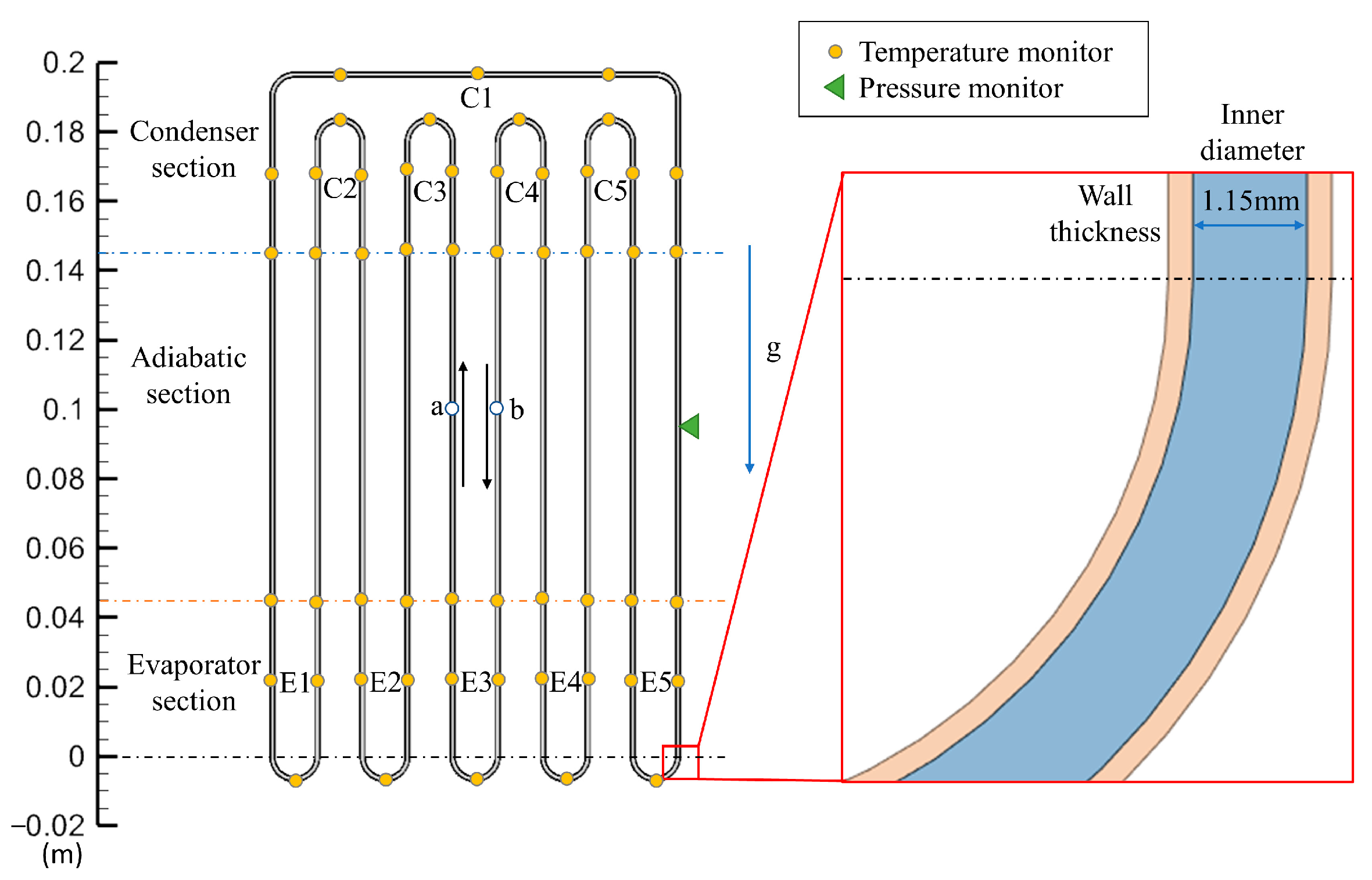
3. Experimental Parameters and Geometry Model

3.1. Experimental Conditions

The geometric features of the PHP that we studied in the previous experiment are shown in Figure 2. The experiment was carried out with four and two thermocouples installed on the evaporator and condenser copper plates, respectively. The averages of their readings indicate the evaporator and condenser temperatures, respectively. The pressure sensor installed at room temperature was connected to the adiabatic section through a thin tube, which was also used as the filling pipe. The condenser temperature was kept by a GM cryocooler. It was 19 K at the smaller heat load, and increased when the heat load exceeded a certain value because of the limited cooling capacity of the cryocooler.

3.2. 2D Model for Simulation

The schematic of the 2D model used is shown in Figure 3. The origin of the vertical axis is at the intersection of the bend and vertical pipe in the evaporator. When the fluid circulates clockwise in the whole PHP, the velocity direction is defined as positive. For points a and b, the positive directions are marked and are used to extract velocity. The copper plates and the filling pipe are not included in the model. For each bend, the evaporator and condenser temperature are represented by the average temperature of all the monitoring points for fluids inside the tube.

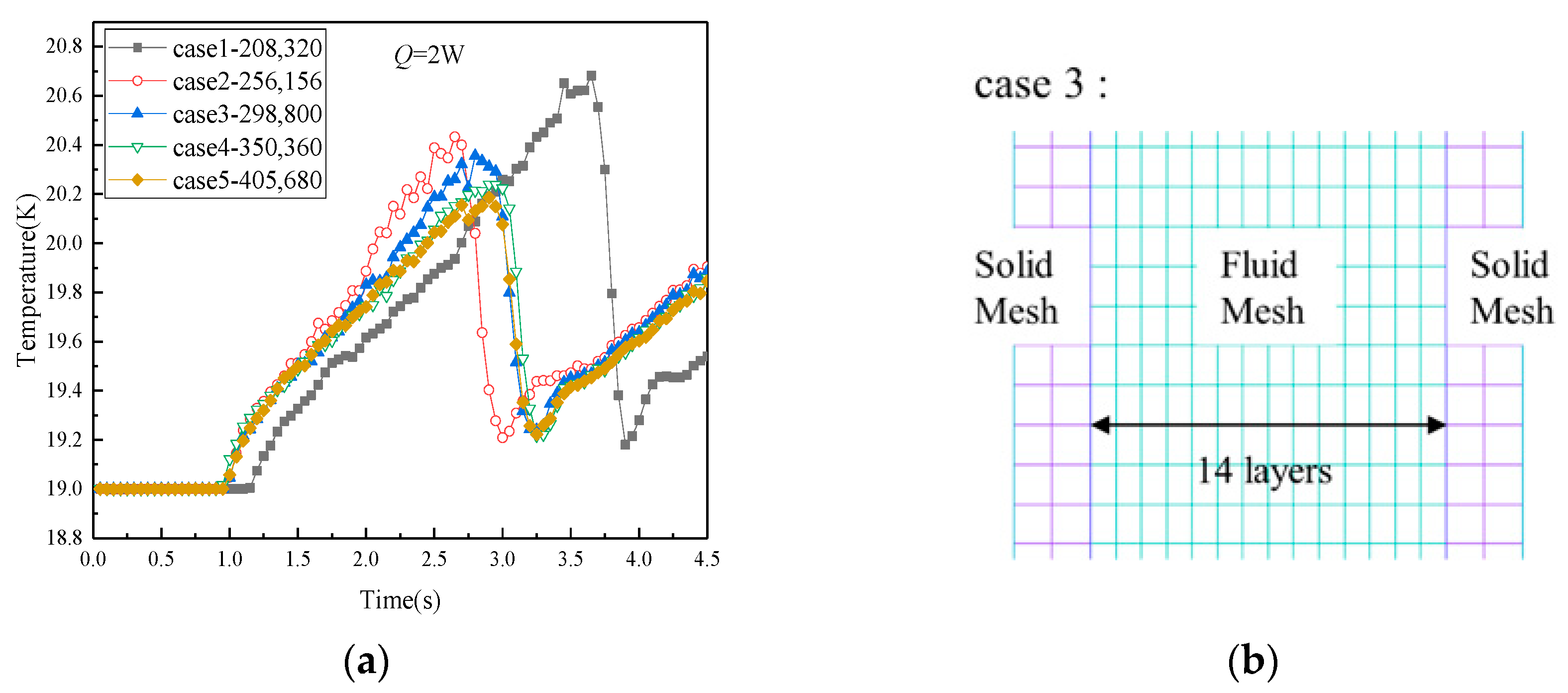
3.3. Grid-Independence and Initial Distribution

When a PHP is partially filled, the working fluid will form randomly distributed, alternating vapor and liquid slugs in the tube due to capillary action. The initial sets and boundary conditions for the simulation are provided in

Table 3. The initial sets and boundary conditions.

Initial Sets	Boundary Conditions
Fluid domain temperature: 19 K Liquid Volume Fraction: 0.51 Pressure: 66,294 Pa	Time	0~0.95 s	0.95~32 s
	Evaporator	19 K	1 W	2 W	3.2 W	3.6 W	4 W	5 W
	Condenser	19 K	19 K	19 K	19.1 K	19.4 K	20.4 K	23.1 K

. To obtain the initial interface state, our simulation was initialized with the condenser temperature, and the pressure inside the channel was the saturation value corresponding to the initial temperature. The boundary conditions for the outer wall of the whole PHP were set to the condenser temperature measured in our experiments for transient calculations until the vapor–liquid phase interface remained stable, which was formed at 0.95 s. Then, the condenser temperature was kept constant, and the boundary conditions for the outer wall of the evaporator and adiabatic section were set to a constant heat load and adiabatic, respectively. The initial liquid filling ratio was 51%.

The numbers of the grids with hexahedral mesh used for the independence test were 208,320, 256,156, 298,800, 350,360 and 405,680, respectively. The dependence of the average temperature in the whole evaporator section on the number of grids is demonstrated in Figure 4. Since the initial vapor–liquid phase interface formed during 0 to 0.95 s, the evaporator temperatures of the five grids were all 19 K. The heat load was 2 W for the simulations with five grids after 0.95 s. As depicted in Figure 4a, the temperature fluctuations in cases 3, 4, and 5 were basically consistent, with a temperature difference of 0.2 K between the highest temperature of case 3 and that of case 5. It is widely accepted that a Courant number less than 1 is advantageous for observing flow characteristics and ensures numerical solution stability. In our simulations, we aimed to maintain a Courant number of approximately 0.5 with a time step of 10⁻⁴ s. Combining this objective with the consideration of computational time cost, we have decided to utilize case 3. Therefore, we opted to utilize case 3.

For case 3, the grid was divided into small and uniform meshes, as illustrated in Figure 4b. It consisted of 14 layers in the radial direction, with an aspect ratio of about 1.25. This mesh configuration enabled the generation of smooth phase interfaces and mitigated the roughness that can arise from excessively wide cells in the center. The simulations were performed using an AMD EPYC 7742 64-core processor. With the utilization of 16 cores, the calculations for a duration of 1 s could be completed within a day for case 3. The simulations used ANSYS Fluent v18.0.

4. Results and Discussion

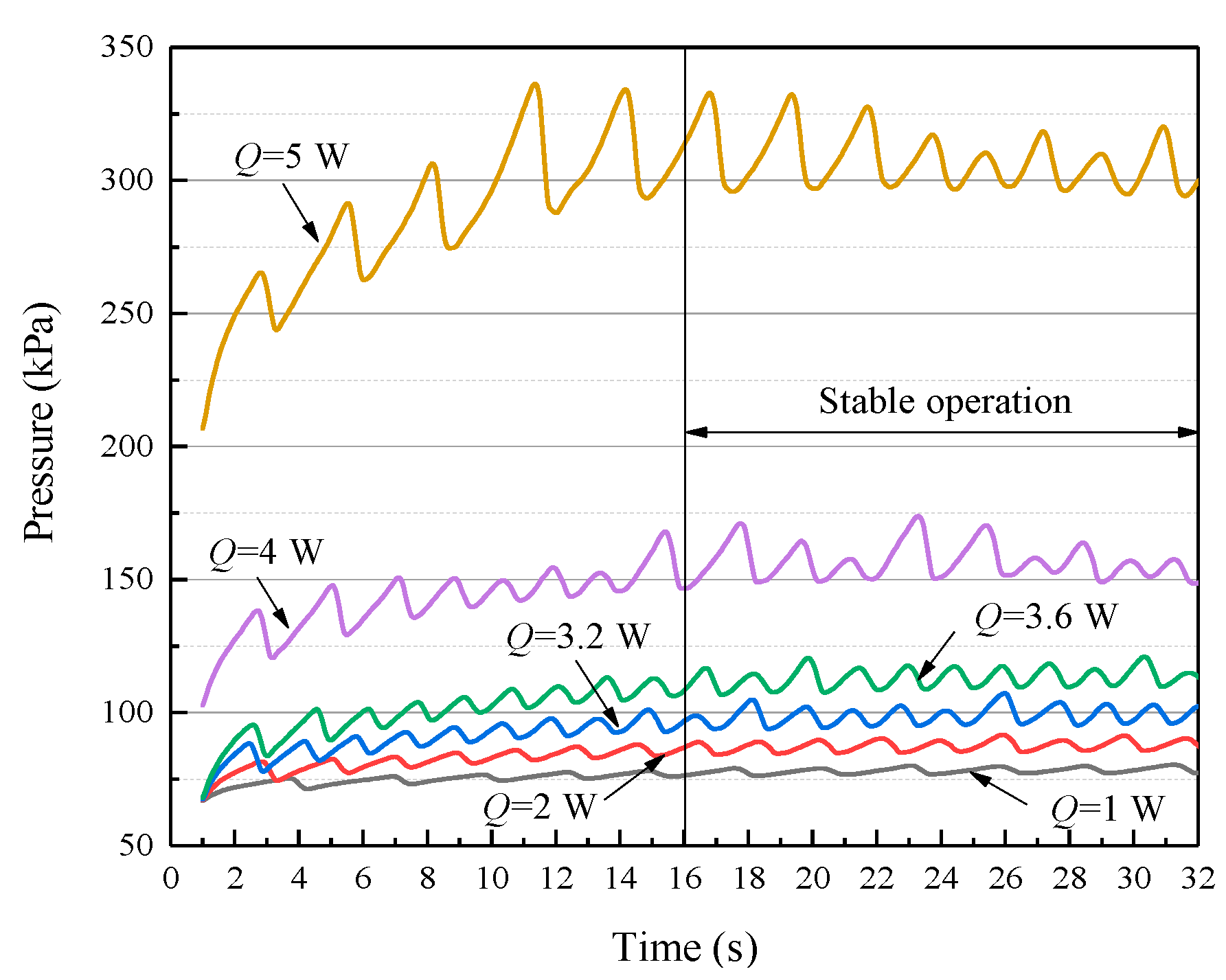
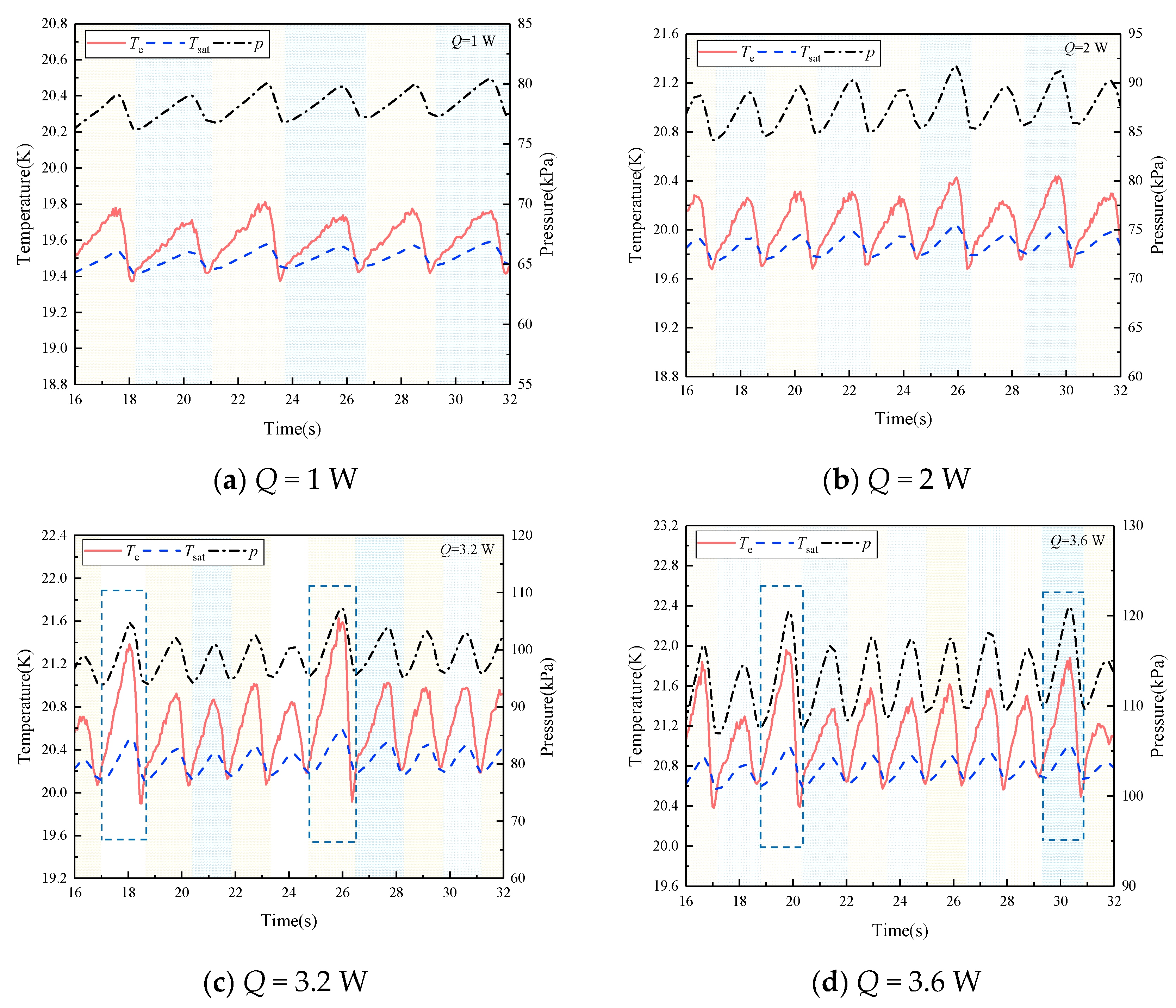
4.1. Comparison between Simulation and Experiment

Once the initial phase interface was stable, the heat load was added at the evaporator after 0.95 s. This led to heat transfer and the changes in pressure over time. In the start-up period, the pressure rises while undergoing oscillations. Subsequently, it fluctuates within a certain range, with the amplitude increasing along with the heat load. Figure 5 shows that the time required for the pressure to achieve stable fluctuation is different at different heat loads. After 16 s, the pressures at the six heat loads all behaved periodically. In order to provide a unified time for analyzing stable performance, the period from 16 s to 32 s was regarded as the period of stable operation.

Figure 6 shows the simulations on the temperature and pressure in stable operation. T_e is the average value of all the monitoring points in evaporator (E1~E5). It can be clearly seen that the oscillations of evaporator temperature and pressure occurred simultaneously. They had a similar oscillation cycle, which is defined by the period between two adjacent minimum values and indicated by the alternating backgrounds. The saturation temperatures T_sat corresponding to the pressures are also given in Figure 6. It can be seen that the evaporator temperatures were mostly above the saturation value. Therefore, the liquid slugs evaporated and bubbles were superheated in the evaporator. This phenomenon provides the power for the PHP to transfer heat to the condenser against gravity.

The oscillations of evaporator temperature and pressure exhibited a higher degree of regularity at the heat loads of 1 W and 2 W. The amplitudes in different cycles were close to each other, as shown in Figure 6a,b. When the heat load reached 3 W, the amplitudes in some cycles were larger than the others, which are circled by the dashed box in Figure 6c,d. As the heat load increased further, the amplitudes in different cycles become obviously different, although they were still in a certain range, as shown in Figure 6e,f. With the progressive increment in heat load, the oscillations of temperature and pressure became more chaotic, which represents the inherent characteristics of a PHP.

Figure 7 illustrates the comparisons between the average values of the simulated and experimental evaporator pressure, temperature, and thermal resistance in the stable operation. The simulated T_e and p were the average values during 16 s~32 s, as shown in Figure 6. The experimental T_e, p, and T_c have been reported in the previous study [30,31]. In our simulations, T_c was the same as the experimental data, which was also the boundary condition for the condenser. This was 19 K at 1 W, 2 W, and 3.2 W, while it increased to 19.4 K, 20.4 K, and 23.1 K at 3.6 W, 4 W, and 5 W, respectively, due to the limitation of the cooling capacity of the cryocooler in the experiment. The simulated temperatures of the fluid in the condenser section (T_c,fluid) are also provided in Figure 7b. In Figure 7c, the experimental thermal resistance was determined by the temperature difference between the average wall temperatures in the evaporator and condenser sections measured in the experiments (T_e − T_c). The simulated thermal resistance was calculated based on the average temperature difference of the fluid (T_e,fluid − T_c,fluid) in the evaporator and condenser sections. It can be observed that the simulations and experimental results showed good agreement in terms of the average pressure, temperature, and thermal resistance.

The higher simulated values of pressure and temperature compared to the experimental values were primarily due to several factors such as the ideal gas assumption, errors in the fit function of the fluid, laminar flow assumptions, and simplifications of the phase change conditions. Figure 7d shows the dependence of the saturation pressure on temperature under two models. The saturation temperature was between 19 K and 25 K, as shown in Figure 6. The maximum difference in saturation pressure between the ideal gas model and the real gas model was approximately 50 kPa, with the ideal gas model yielding higher values than the real gas model at 25 K. From Figure 7b, the temperature difference of the fluid in the evaporator and condenser sections (T_e,fluid − T_c,fluid) was smaller than that of the wall surfaces measured in the experiments (T_e − T_c). The errors in temperature and pressure are shown in

Table 4. Errors between the simulated and experimental results.

Q (W)	Error of P (%)	Error of Te (%)
1	16.26	1.75
2	21.96	2.85
3.2	22.12	3.54
3.6	22.92	3.84
4	23.69	4.81
5	23.71	4.69

. As a result, this led to smaller thermal resistance values in the simulation (see Figure 7c). Although the error of the CFD simulation was larger than that of the previous one-dimensional numerical simulation, the CFD simulation was still able to represent more flow characteristics. In addition, the trend of the simulations matched that of the experiments better compared to the one-dimensional model developed by our team previously.

4.2. The Evaporation and Condensation Inside the PHP

CFD simulation can obtain the flow pattern and two-phase interface, which can demonstrate the evaporation and condensation inside a PHP. Taking the channels C4 and E4 as an example, Figure 8 shows the evolution of vapor–liquid distribution with time in condenser when the heat load is added. It can be seen that the two vapor plugs (1, 3) and a long vapor plug (2) through the tube bend keep shrinking, as well as the ones (4, 5) entering condenser. They all have the smooth and regular phase interface during condensation, except for one vapor plug at 2.50 s, which is caused by the merging of two vapor plugs (3, 4) at 2.25 s.

Figure 9 illustrates the evolution of vapor–liquid distribution in evaporator during the same time. In the period of 1~2 s, it can be found that bubbly flow is gradually formed by the continuous small bubbles appearing in the liquid slug. Because of the bubbles growth and combination, the bubble diameter gradually approaches the pipe diameter and begins to elongate during the period of 2~3 s, and the flow pattern changes to slug flow. In this process, bubbles merge frequently, and the vapor plug also expands, resulting in the rough phase interface. The irregularity caused by bubbles merging is more prominent, which is also circled in Figure 9.

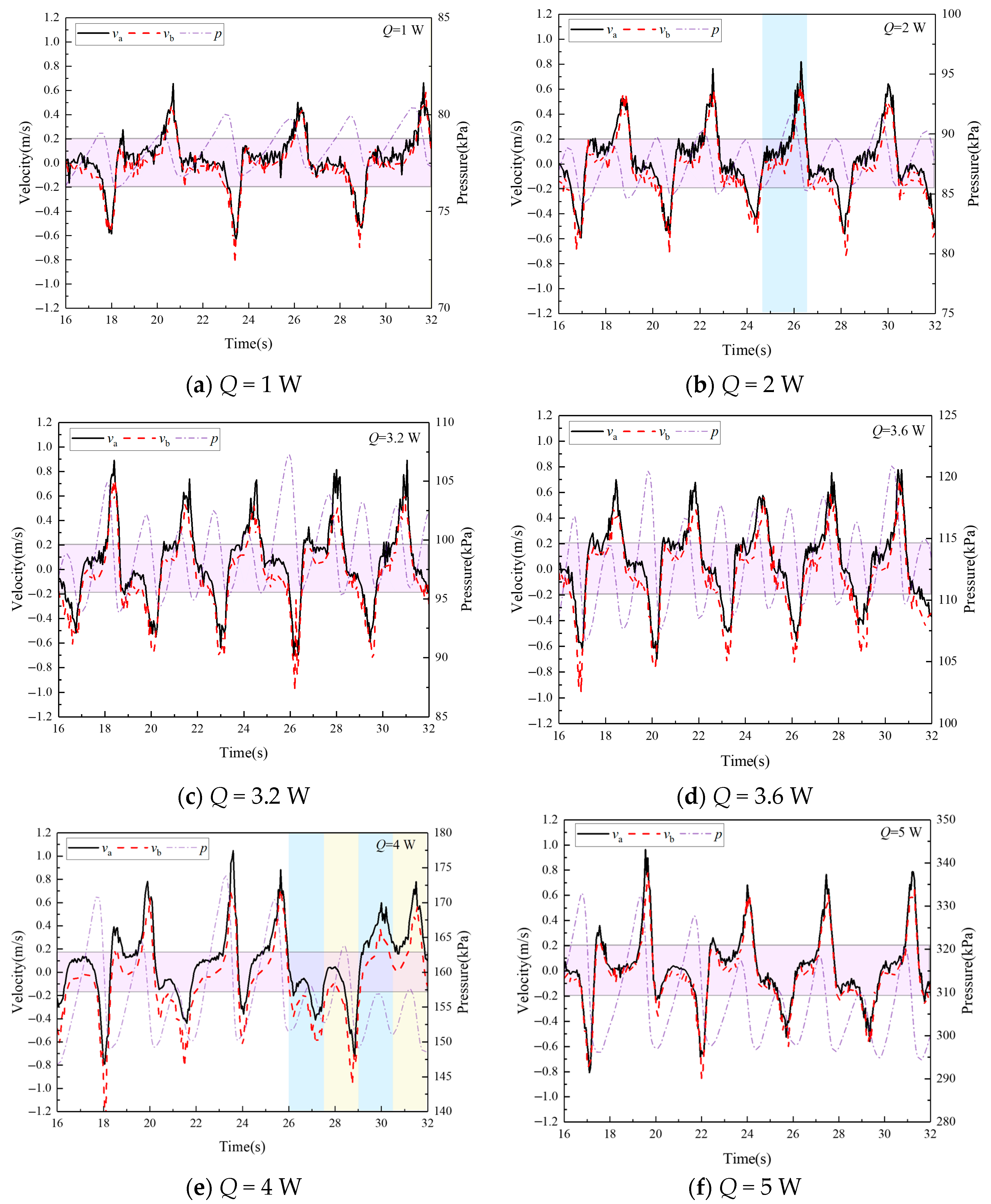
4.3. The Velocity Characteristics in the Stable Operation

In the simulation results, the velocity differences between different points keep almost constant. The phase change in evaporator and condenser can produce instantaneous disturbance, which will affect the analysis of the overall motion. Therefore, two points a and b in adiabatic section, shown in Figure 3, are selected for analyzing the velocity characteristics. The relations between pressure and velocity in the stable operation are illustrated in Figure 10. At the six different heat loads, flow reversals between the continuous oscillation cycles of pressure are observed, with the exception of the cycles occurring from 26 s to 32 s at 4 W. It can be obviously found that there is a period in each cycle, in which the velocity fluctuates slightly around a certain value. As shown by the pink box in Figure 10, this certain value generally remains in the range of 0.2~0.2 m/s which is defined as the uniform velocity stage. The velocity in the rest time in each cycle has larger acceleration.

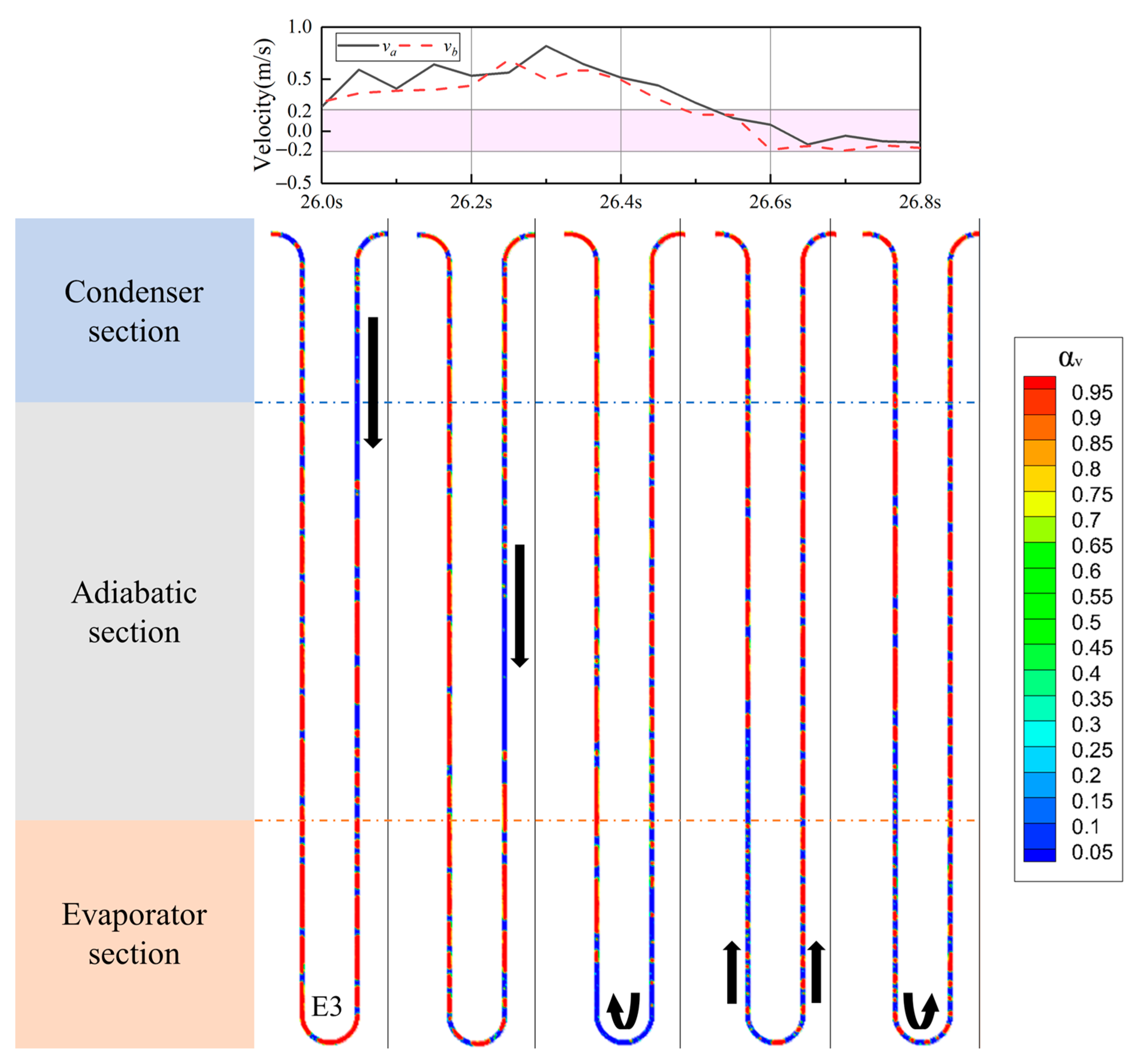
4.4. The Vapor–Liquid Distribution

In order to learn the reasons for the velocity characteristics, the performances of fluid flow in channel E3 during 24.8~26.8 s at 2 W, as seen in Figure 10b, were adopted to analyze the vapor–liquid distribution. Figure 11 reveals that the channel primarily consisted of vapor plugs at 24.8 s. As a result, the liquid slugs between the vapor plugs were very short, and there was enough surface tension to support the liquid slugs to maintain balance. Consequently, the liquid and vapor plugs oscillated slightly near their respective positions. From 25.4 s to 25.8 s, it can be observed that a longer liquid slug gradually formed in the right channel of the condenser due to the continuous condensation. Finally, the surface tension could not balance the gravity of the long liquid slug, leading to the termination of the uniform velocity stage.

As shown in Figure 12, the long liquid slug in the right channel of the condenser flowed rapidly toward the evaporator, and consequently, the vapor plugs in the evaporator were pushed into the adiabatic section in the left channel. The arrows mark the motion of the liquid slug. At 26.4 s, the long liquid slug flowed through the bend of the evaporator, and the reduction in the gravity effect made the flow clockwise slow, causing deceleration. At the same time, small bubbles occurred in the liquid slug. At 26.6 s, the bubbles in the right channel of the evaporator had grown into vapor plugs. After 26.8 s, the fluid entered the uniform velocity stage again. Because the liquid slug in the left channel of the evaporator was longer, the effect of gravity on it was greater than that in the right channel. Therefore, the next uniform stage will be formed at a very small velocity anticlockwise. In the uniform velocity stage, the liquid and vapor plugs oscillated slightly near their respective positions. Therefore, the convective heat transfer was weak and the latent heat transfer was strong. When the velocity was large, the liquid and vapor plugs were kept in the condenser and evaporator for a short time, forming flow circulation in the channel. As a result, convective heat transfer plays a more important role. Through the IR measurements, Pagliarini et al. observed two flow patterns in the PHP: intermittent flow and full activation [32,33], which are similar to the two flow patterns analyzed in this section.

When the velocity was smaller than 0.6 m/s inside the PHP, the advancing and receding contact angles of the liquid slug were close to each other (see Figure 9). The arrows mark the motion of the working fluid. When the velocity was larger than 0.6 m/s, dynamic contact angle hysteresis was observed in the condenser. When the heat load was in the range of 3.2 W~5 W (see Figure 13), it can be clearly found that the curvature of the phase interface at advancing was larger than that at receding, which has been obtained in some visualization studies [26,34]. According to Equation (7), the greater the curvature of the interface, the greater the surface tension. Under these conditions, the cumulative effect of surface tension opposes the motion of the working fluid. The additional resistance is proportional to the number of liquid slugs. Therefore, it can be concluded that more liquid slugs can result in larger flow resistance at larger velocities. In the evaporator, bubbles were formed and merged frequently, and a stable interface hardly occurred. As a result, the phenomenon was not observed.

5. Conclusions

A 2D model, based on the VOF method and Lee model, was established to analyze the heat transfer and flow performance of a hydrogen PHP with five turns. The values of β_e and β_c were set to 5 and 500, respectively. The initial filling ratio was 51%, and the condenser temperature was set to the values measured in the experiments, which were 19~23 K at different heat loads. The comparisons between the simulation and our experiment, which has been previously performed, were carried out regarding the average values of the pressure, evaporator temperature, and thermal resistance in the stable operation. Its validity was confirmed by the consistent agreement. The simulation results indicate that the maximum errors of pressure and temperature were 23.71% and 4.81%, respectively.

In the stable operation, the simulation results revealed that the oscillations of the evaporator temperature and pressure were synchronous. The evaporator temperatures were mostly above the saturation values, according to the pressures, which indicates that the vapor plugs were superheated. Each oscillation cycle comprised a uniform velocity stage where the working fluid oscillated at a low velocity, followed by a significant increase in velocity. Moreover, there were almost flow reversals between the continuous oscillation cycles. These phenomena can be attributed to the movement of the long liquid slug formed in the condenser and the separation of the long liquid slug by the generated bubbles due to evaporation. In addition, when the velocity was greater than 0.6 m/s, dynamic contact angle hysteresis was observed in the condenser, which causes additional resistance to fluid flow.

It should be noted that the assumptions of an ideal gas and constant latent heat were employed in our model, which simplified the physical properties of real fluids. This simplification introduces uncertainty into the simulation results. Additionally, the coefficients of the Lee model were assumed to be constant, which have an impact on the accuracy of the results. In future research, efforts will be made to address these limitations and improve the model.

References

1. Andersson, J.; Grönkvist, S. Large-scale storage of hydrogen. Int. J. Hydrog. Energy 2019, 44, 11901–11919. [Google Scholar] [CrossRef]
2. Al Ghafri, S.Z.; Munro, S.; Cardella, U.; Funke, T.; Notardonato, W.; Trusler, J.M.; Leachman, J.; Span, R.; Kamiya, S.; Pearce, G. Hydrogen liquefaction: A review of the fundamental physics, engineering practice and future opportunities. Energy Environ. Sci. 2022, 15, 2690–2731. [Google Scholar] [CrossRef]
3. Notardonato, W.; Baik, J.; McIntosh, G. Operational Testing of Densified Hydrogen Using G-M Refrigeration. AIP Conf. Proceeding 2004, 170, 664–674. [Google Scholar]
4. Notardonato, W.; Swanger, A.; Fesmire, J.; Jumper, K.; Johnson, W.; Tomsik, T. Zero boil-off methods for large-scale liquid hydrogen tanks using integrated refrigeration and storage. IOP Conf. Ser. Mater. Sci. Eng. 2017, 278, 012012. [Google Scholar] [CrossRef]
5. Hastings, L.J.; Plachta, D.; Salerno, L.; Kittel, P. An overview of NASA efforts on zero boiloff storage of cryogenic propellants. Cryogenics 2001, 41, 833–839. [Google Scholar] [CrossRef]
6. Plachta, D.; Stephens, J.; Johnson, W.; Zagarola, M. NASA cryocooler technology developments and goals to achieve zero boil-off and to liquefy cryogenic propellants for space exploration. Cryogenics 2018, 94, 95–102. [Google Scholar] [CrossRef]
7. Wan, C.; Zhu, S.; Shi, C.; Bao, S.; Zhi, X.; Qiu, L.; Wang, K. Numerical simulation on pressure evolution process of liquid hydrogen storage tank with active cryogenic cooling. Int. J. Refrig. 2023, 150, 47–58. [Google Scholar] [CrossRef]
8. Faraji, H.; Yıldız, Ç.; Arshad, A.; Arıcı, M.; Choukairy, K.; El Alami, M. Passive thermal management strategy for cooling multiple portable electronic components: Hybrid nanoparticles enhanced phase change materials as an innovative solution. J. Energy Storage 2023, 70, 108087. [Google Scholar] [CrossRef]
9. Winkler, M.; Vergez, M.; Mahlke, A.; Gebauer, M.; Müller, P.; Reising, C.; Bartholomé, K.; Schäfer-Welsen, O. Flat-Plate PHP with Gravity-Independent Performance and High Maximum Thermal Load. Energies 2023, 16, 7463. [Google Scholar] [CrossRef]
10. Sun, Q.; Qu, J.; Li, X.; Yuan, J. Experimental investigation of thermo-hydrodynamic behavior in a closed loop oscillating heat pipe. Exp. Therm. Fluid Sci. 2017, 82, 450–458. [Google Scholar] [CrossRef]
11. Ayel, V.; Slobodeniuk, M.; Bertossi, R.; Romestant, C.; Bertin, Y. Flat plate pulsating heat pipes: A review on the thermohydraulic principles, thermal performances and open issues. Appl. Therm. Eng. 2021, 197, 117200. [Google Scholar] [CrossRef]
12. Mameli, M.; Besagni, G.; Bansal, P.K.; Markides, C.N. Innovations in pulsating heat pipes: From origins to future perspectives. Appl. Therm. Eng. 2022, 203, 117921. [Google Scholar] [CrossRef]
13. Mushan, S.G.; Deshmukh, V.N. A review of pulsating heat pipes encompassing their dominant factors, flexible structure, and potential applications. Int. J. Green Energy 2024, 1–38. [Google Scholar] [CrossRef]
14. Pfotenhauer, J.M.; Sun, X.; Berryhill, A.; Shoemaker, C.B. The influence of aspect ratio on the thermal performance of a cryogenic pulsating heat pipe. Appl. Therm. Eng. 2021, 196, 117322. [Google Scholar] [CrossRef]
15. Li, M.N.; Li, L.F.; Xu, D. Effect of filling ratio and orientation on the performance of a multiple turns helium pulsating heat pipe. Cryogenics 2019, 100, 62–68. [Google Scholar] [CrossRef]
16. Liang, Q.; Fang, C.; Li, Y.; Liu, J.; Zhao, W.; Ai, L. Cooldown characteristics of a neon cryogenic pulsating heat pipe. J. Low Temp. Phys. 2022, 207, 278–294. [Google Scholar] [CrossRef]
17. Dixit, T.; Authelet, G.; Mailleret, C.; Gouit, F.; Stepanov, V.; Baudouy, B. High performance and working stability of an 18 W class neon pulsating heat pipe in vertical/horizontal orientation. Cryogenics 2023, 132, 103670. [Google Scholar] [CrossRef]
18. Mueller, B.; Pfotenhauer, J.; Miller, F. Performance of nitrogen pulsating heat pipes as passive thermal switches in a redundant cryocooler application. Appl. Therm. Eng. 2021, 196, 117213. [Google Scholar] [CrossRef]
19. Li, S.Z.; Bu, Z.C.; Fang, T.G.; Wang, Y.; Shen, Y.; Tao, X.; Jiao, B.; Gan, Z. Experimental study on the thermo-hydrodynamic characteristics of a nitrogen pulsating heat pipe. Int. Commun. Heat Mass Transf. 2023, 146, 106920. [Google Scholar] [CrossRef]
20. Sun, X.; Li, S.; Jiao, B.; Gan, Z.; Pfotenhauer, J.; Wang, B.; Zhao, Q.; Liu, D. Experimental study on hydrogen pulsating heat pipes under different number of turns. Cryogenics 2020, 111, 103174. [Google Scholar] [CrossRef]
21. Chandratilleke, R.; Hatakeyama, H.; Nakagome, H. Development of cryogenic loop heat pipes. Cryogenics 1998, 38, 263–269. [Google Scholar] [CrossRef]
22. Natsume, K.; Mito, T.; Yanagi, N.; Tamura, H.; Tamada, T.; Shikimachi, K.; Hirano, N.; Nagaya, S. Heat transfer performance of cryogenic oscillating heat pipes for effective cooling of superconducting magnets. Cryogenics 2011, 51, 309–314. [Google Scholar] [CrossRef]
23. Mito, T.; Natsume, K.; Yanagi, N.; Tamura, H.; Terazaki, Y. Enhancement of thermal properties of HTS magnets using built-in cryogenic oscillating heat pipes. IEEE Trans. Appl. Supercond. 2013, 23, 4602905. [Google Scholar] [CrossRef]
24. Lemmon, E.W.; Huber, M.L.; McLinden, M.O. NIST Standard Reference Database 23; National Institute of Standards and Technology: Gaithersburg, MD, USA, 2010. [Google Scholar]
25. Shafii, M.B.; Faghri, A.; Zhang, Y.W. Thermal modeling of unlooped and looped pulsating heat pipes. J. Heat Transf. -Trans. ASME 2001, 123, 1159–1172. [Google Scholar] [CrossRef]
26. Nikolayev, V.S. Physical principles and state-of-the-art of modeling of the pulsating heat pipe: A review. Appl. Therm. Eng. 2021, 195, 117111. [Google Scholar] [CrossRef]
27. Mucci, A.; Kholi, F.K.; Chetwynd-Chatwin, J.; Ha, M.Y.; Min, J.K. Numerical investigation of flow instability and heat transfer characteristics inside pulsating heat pipes with different numbers of turns. Int. J. Heat Mass Transf. 2021, 169, 120934. [Google Scholar] [CrossRef]
28. Dreiling, R.; Dubois, V.; Zimmermann, S.; Nguyen-Xuan, T.; Schreivogel, P.; di Mare, F. Numerical investigation of slug flow in pulsating heat pipes using an interface capturing approach. Int J Heat Mass Transf. 2022, 199, 123459. [Google Scholar] [CrossRef]
29. Liu, Y.; Dan, D.; Wei, M.; Zheng, S.; Sun, J. Numerical investigation on the start-up and heat transfer performance of dual-diameter pulsating heat pipes. Appl. Therm. Eng. 2024, 236, 121709. [Google Scholar] [CrossRef]
30. Sun, X.; Li, S.Z.; Wang, B.; Jiao, B.; Pfotenhauer, J.; Miller, F.; Gan, Z. Numerical study of the thermal performance of a hydrogen pulsating heat pipe. Int. J. Therm. Sci. 2022, 172, 107302. [Google Scholar] [CrossRef]
31. Gan, Z.H.; Sun, X.; Jiao, B.; Han, D.; Deng, H.; Wang, S.; Pfotenhauer, J.M. Experimental Study on a Hydrogen Closed Loop Pulsating Heat Pipe with Different Adiabatic Lengths. Heat Transf. Eng. 2019, 40, 205–214. [Google Scholar] [CrossRef]
32. Pagliarini, L.; Cattani, L.; Bozzoli, F.; Mameli, M.; Filippeschi, S.; Rainieri, S.; Marengo, M. Thermal characterization of a multi-turn pulsating heat pipe in microgravity conditions: Statistical approach to the local wall-to-fluid heat flux. Int. J. Heat Mass Transf. 2021, 169, 120930. [Google Scholar] [CrossRef]
33. Iwata, N.; Bozzoli, F.; Pagliarini, L.; Cattani, L.; Vocale, P.; Malavasi, M.; Rainieri, S. Characterization of thermal behavior of a micro pulsating heat pipe by local heat transfer investigation. Int. J. Heat Mass Transf. 2022, 196, 14. [Google Scholar] [CrossRef]
34. Blasiak, P.; Opalski, M.; Parmar, P.; Czajkowski, C.; Pietrowicz, S. The Thermal-Flow Processes and Flow Pattern in a Pulsating Heat Pipe-Numerical Modelling and Experimental Validation. Energies 2021, 14, 5952. [Google Scholar] [CrossRef]
Figure 1. Schematic of a closed-loop PHP.
Energies 17 02697 g001
Figure 2. Schematic of the experimental setup [20].
Energies 17 02697 g002
Figure 3. Schematic of the 2D PHP in our simulation.
Energies 17 02697 g003
Figure 4. The curve of the evaporator temperature with 0~4.5 s (a) and the mesh layer of case 3 (b).
Energies 17 02697 g004
Figure 5. The dependence of the simulated pressure on time at different heat loads.
Energies 17 02697 g005
Figure 6. The temperatures and pressures in the stable operation.
Energies 17 02697 g006aEnergies 17 02697 g006b
Figure 7. Comparisons between the average values of the experiment and simulation in stable operation: (a) pressure; (b) temperature; (c) thermal resistance; (d) saturation pressure vs. saturation temperature of hydrogen.
Energies 17 02697 g007
Figure 8. Condensation of gas plug in condenser.
Energies 17 02697 g008
Figure 9. Bubble growth and flow pattern transition in evaporator.
Energies 17 02697 g009
Figure 10. The velocity characteristics in the stable operation.
Energies 17 02697 g010
Figure 11. Vapor–liquid distribution during 24.8~25.8 s at Q = 2 W.
Energies 17 02697 g011
Figure 12. Vapor–liquid distribution during 26.0~26.8 s at Q = 2 W.
Energies 17 02697 g012
Figure 13. The phase interface at higher velocities.
Energies 17 02697 g013