Techno-Economic Assessment of Molten Salt-Based Concentrated Solar Power: Case Study of Linear Fresnel Reflector with a Fossil Fuel Backup under Saudi Arabia’s Climate Conditions

Abstract

Concentrated solar power (CSP) has gained traction for generating electricity at high capacity and meeting base-load energy demands in the energy mix market in a cost-effective manner. The linear Fresnel reflector (LFR) is valued for its cost-effectiveness, reduced capital and operational expenses, and limited land impact compared to alternatives such as the parabolic trough collector (PTC). To this end, the aim of this study is to optimize the operational parameters, such as the solar multiple (SM), thermal energy storage (TES), and fossil fuel (FF) backup system, in LFR power plants using molten salt as a heat transfer fluid (HTF). A 50 MW LFR power plant in Duba, Saudi Arabia, serves as a case study, with a Direct Normal Irradiance (DNI) above 2500 kWh/m². About 600 SM-TES configurations are analyzed with the aim of minimizing the levelized cost of electricity (LCOE). The analysis shows that a solar-only plant can achieve a low LCOE of 11.92 ¢/kWh with a capacity factor (CF) up to 36%, generating around 131 GWh/y. By utilizing a TES system, the SM of 3.5 and a 15 h duration TES provides the optimum integration by increasing the annual energy generation (AEG) to 337 GWh, lowering the LCOE to 9.24 ¢/kWh, and boosting the CF to 86%. The techno-economic optimization reveals the superiority of the LFR with substantial TES over solar-only systems, exhibiting a 300% increase in annual energy output and a 20% reduction in LCOE. Additionally, employing the FF backup system at 64% of the turbine’s rated capacity boosts AEG by 17%, accompanied by a 5% LCOE reduction. However, this enhancement comes with a trade-off, involving burning a substantial amount of natural gas (503,429 MMBtu), leading to greenhouse gas emissions totaling 14,185 tonnes CO₂ eq. This comprehensive analysis is a first-of-a-kind study and provides insights into the optimal designs of LFR power plants and addresses thermal, economic, and environmental considerations of utilizing molten salt with a large TES system as well as employing natural gas backup. The outcomes of the research address a wide audience including academics, operators, and policy makers.

1. Background

Researchers are exploring lowering the cost of clean-energy-generated power to accelerate the transition to renewable energy [1,2,3,4]. Between 2010 and 2021, utility-scale solar PV projects experienced a global weighted average LCOE fall of 88%, outpacing reductions in onshore wind, offshore wind, and CSP (by about 68%) [5]. In 2021, the cost of electricity generated by CSP plants dropped to less than 0.1 $/kWh [6]. Until 2021, operational CSP plants have a cumulative capacity of around 6.7 GW [7]. The PTC is the most mature, with 76.6%, followed by the SPT and LFR (only around 8%) [8].

The LFR is a cost-reduction alternative for the parabolic trough collector in CSP due to its simpler design [9]. It has minimal capital and maintenance costs, low materials demand, and minimal land usage [10]. The LFR offers sufficient thermodynamic performance while avoiding economic and technological challenges, such as ground preparation and tower heights [11]. However, it has several thermodynamic drawbacks, including lower optical and conversion efficiencies, lower output steam temperatures, high cosine losses, and a lower concentration ratio compared to other CSP types [10,11,12,13]. Since the SF’s outlet temperature is relatively low compared to the point focusing technique, the LFR is known as a suitable option for direct steam generation; however, recently, it has exhibited a promising capacity to utilize different HTF to produce steam indirectly at higher temperatures [14,15,16,17].

1.1. Molten Salt

The utilization of molten salt (MS) in conjunction with the LFR approach has been demonstrated as an effective option for achieving an optical efficiency of up to 55% [14]. The LFR is known as a form of CSP that generates medium-temperature steam up to 400 °C, but thanks to the molten salt characteristics, it could reach as high as 565 °C in certain conditions [15,18]. There are several types of MS and the most suitable types that are utilized in LFR applications due to their highest working temperatures are Hitec Solar Salt $(60\mathrm{\%} {\mathrm{N}\mathrm{A}\mathrm{N}\mathrm{O}}_3+40\mathrm{\%} {\mathrm{K}\mathrm{N}\mathrm{O}}_3)$, Hitec $\left(7\mathrm{\%} {\mathrm{N}\mathrm{A}\mathrm{N}\mathrm{O}}_3+53\mathrm{\%} {\mathrm{K}\mathrm{N}\mathrm{O}}_3+40\mathrm{\%} {\mathrm{N}\mathrm{a}\mathrm{N}\mathrm{O}}_2\right)$, and $\left(7\mathrm{\%} {\mathrm{N}\mathrm{A}\mathrm{O}}_3+45\mathrm{\%} {\mathrm{K}\mathrm{N}\mathrm{O}}_3+48\mathrm{\%} {\mathrm{C}\mathrm{a}(\mathrm{N}\mathrm{O}}_3{)}_2\right)$ [18,19,20]. Hitec Solar Salt was chosen in this investigation due to its capacity to reach temperatures of up to about 600 °C [18]. Additionally, Hitec and Hitec XL fail to offer the same outstanding thermal stability as Solar Salt, while having lower freezing points [21].

1.2. Thermal Energy Storage

The solar field is a significant expense in CSP power plants, accounting for approximately 35–50% of the total costs [22,23]. The expenses of the SF include various components of the LFR system, along with land expenditures, site enhancements, and labor. Considering the low capital cost of solar fields in LFR technology, TES can be used to increase the overall power plant performance [24]. Integrating thermal energy storage with concentrated solar power technologies improves system stability and maximizes production at high loads [25]. Despite the fact that the TES may incur charges when power generation exceeds demand, it is being regarded by numerous researchers as a technology with high costs [26]. Hence, according to the findings of the study [27], it has been suggested that a smaller thermal energy storage (TES) size may result in the lowest LCOE for LFR technology. However, recently, the new under-structure projects are using two-indirect MS storage tanks with bigger sizes [28]. The TES exhibits promising potential for surpassing other storage methods due to its superior efficiency and its occurrence prior to the conversion of mechanical and electrical energy. As a result, TES has recently been used on the latest commercial power plants because of its ability to obtain a higher CF of the LFR power plants. In 2022, worldwide operational projects utilized about 10 GW of the larger TES [7]. The TES becomes a crucial subsystem component of CSP, with molten salt predicted to be used in 67% of the CSP projects and just 30% of the power plants without storage [7]. Nonetheless, the primary challenges associated with thermal energy storage revolve around capital investment and storage capacity [9]. Other researchers argued that the implementation of a hybrid system, which incorporates suitable energy storage facilities, has resulted in a notable reduction in the overall cost associated with the increase in energy production [29]. This technical improvement has the potential to reduce the LCOE [30]. Thus, it is imperative to optimize the optimal size of the TES system and the necessary SF area.

1.3. Solar Multiple Thermal Energy Storage Parametric Analysis

Researchers use the solar multiple term, which is the ratio of thermal power generated via the SF at the design point to the thermal power required by the Power Block (PB) [31]. For instance, Montes et al. [31] optimized the SM of a solar-only PTC power plant by using five-year average monthly metrological data at a location in Spain and concluded that the optimum SM value of 1.16 can operate the power cycle with the lowest LCOE. Sultan et al. [32] investigated different design configurations for PTCs and concluded that the value of 3.3 SM and 15 h of thermal energy storage produce electricity at the lowest cost. Similarly, Alfailakawi et al. [33] investigated the impact of aerosol on the size of the solar field and the TES to determine the optimal layout to achieve the lowest LCOE and discovered that the 3.2 SM and 16 h of storage produce electricity for only 12.87 $(\mathrm{¢}/\mathrm{k}\mathrm{W}\mathrm{h})$.

Regarding the LFR, an examination of a 50 MW LFR power plant in Spain that uses water as the heat transfer fluid, for instance, showed that its optimal design has a larger solar field (SM = 2) with a 2 h TES and 1.7 SM in the case of the absence of thermal energy storage [27]. Mihoub, Sofiane [23] presented a comparative analysis of a 50 MW LFR in different locations in Algeria for multiple cases from the solar-field-only case to a combined design of the solar field, TES, and the fossil fuel backup system, and that the molten-salt LFR plant with 25% of BS and 6 h of TES is the optimum solution. In this analysis, an annual thermal investigation of up to 18 h of the thermal storage capacity with a solar field range of up to 4 coupled with a fossil fuel back up system to reach the highest possible thermal performance and the lowest LCOE.

2. Aim and Objectives

This study aims to validate the capability of molten salt in efficiently operating the LFR solar field, particularly with a large TES, to produce cost-effective electricity. The primary goal is to find optimal configurations for SM and TES capacities while integrating a fossil fuel backup system to maximize thermal performance. Additionally, this study seeks to minimize energy production costs associated with the LFR power plant, ensuring continuous operational functionality. Insights into utilizing molten salt with a large TES system and incorporating natural gas backup, particularly in climates with low water availability and extremely high DNI values (>2500 kWh/m²), are essential components of the aim. The primary objectives of this analysis are as follows:

• Determine optimal SM and TES sizes for the efficient operation of the LFR solar field;
• Integrate a fossil fuel backup system to enhance thermal performance and assess its impact on overall energy production;
• Conduct a detailed investigation into the annual and daily thermal performance of the LFR power plant under varying conditions;
• Minimize energy production costs associated with the LFR power plant while ensuring continuous operational functionality;
• Provide multiple optimum configurations for the solar field, TES, and FF backup sizes to achieve the lowest LCOE and highest thermal performance;
• Offer deeper insights into the utilization of molten salt with a large TES system and the use of a natural gas backup, particularly in climates with specific environmental and meteorological characteristics.

These objectives collectively contribute to a comprehensive understanding of the efficient operation, economic viability, and environmental impact of LFR power plants, specifically focusing on the integration of molten salt, TES, and FF backup systems.

3. Material and Methods

The majority of CSP facilities typically have a capacity of 50 MW. This emphasizes the significance of medium-sized turbine capacity in CSP plants and highlights the expertise of leading countries such as Spain, the United States, and China, which have extensive experience in deploying multiple CSP installations [8,14,34,35]. The commercial deployment of LFR technology is currently limited compared to PTC. LFR plants are presently undergoing construction, development, or are currently offline.

Table 1. Summary of the worldwide operational LFR power plants, their locations, and important parameters.

Power Plant Name	Location	Capacity (MW)	Annual Production (GWh)	HTF	Thermal Storage	Solar Field/Land Area
Dacheng Dunhuang	China–Gansu Province	50	214	Molten Salt	2- tank 13 h Molten Salt	1,270,000 ${\mathrm{m}}^2$
Dhursar	India–Dhursar Rajasthan	125	280	Water/Steam	None	340 hectares
eCare Solar Thermal Project	Morocco	1	1.6	Water/Steam	2 h steam drum	2 hectares
eLLO Solar Thermal Project	France–Llo Pyrénées Orientales	9	20.2	Water/Steam	3 h steam drum	35 hectares 153,000 ${\mathrm{m}}^2$
Puerto Errado 1 Thermosolar	Spain–Calasparra Murcia	1.4	2	Water/Steam	1 Ruths Tank thermocline	5 hectares 18,662 ${\mathrm{m}}^2$
Puerto Errado 2 Thermosolar	Spain–Calasparra Murcia	30	49	Water/Steam	0.5 h 1 Ruths Tank thermocline	70 hectares 302,000 ${\mathrm{m}}^2$
Rende–CSP Plant	Italy–Rende Calabria	1	3	Diathermic Oil	None	2 hectares 9780 ${\mathrm{m}}^2$
Augustin Fresnel-1	Targassonne, France	0.25	-	Water/Steam	0.25 h 1 Ruths Tank thermocline	400 ${\mathrm{m}}^2$
Huaqiang TeraSolar	Zhangbei Zhangjiakou Hebei China	15	75	Water/Steam	14 h Solid State formulated Concrete	170,000 ${\mathrm{m}}^2$
Lanzhou Dacheng Dunhuang	Dunhuang Jiuquan Gansu China	10	60	Molten salt	16 h	0.6 ${\mathrm{k}\mathrm{m}}^2$

presents a comprehensive compilation of major commercially operating LFR power plants across various regions worldwide [9,10,27,28,35,36,37].

Table 1 clearly shows that the majority of operational power plants use water as the heat transfer fluid, with just two employing molten salt. Furthermore, most of them lack TES or have very limited storage (1–3 h). Currently, only two power plants in the world employ molten salt as a thermal storage medium, with a storage capacity of more than 12 h, and both are in China [38]. The power plant under consideration and validation in this study is the Dacheng Dunhuang power plant, with a capacity of 50 MW. Notably, this power plant is equipped with a thermal energy storage system capable of storing thermal energy for a duration of 13 h [39].

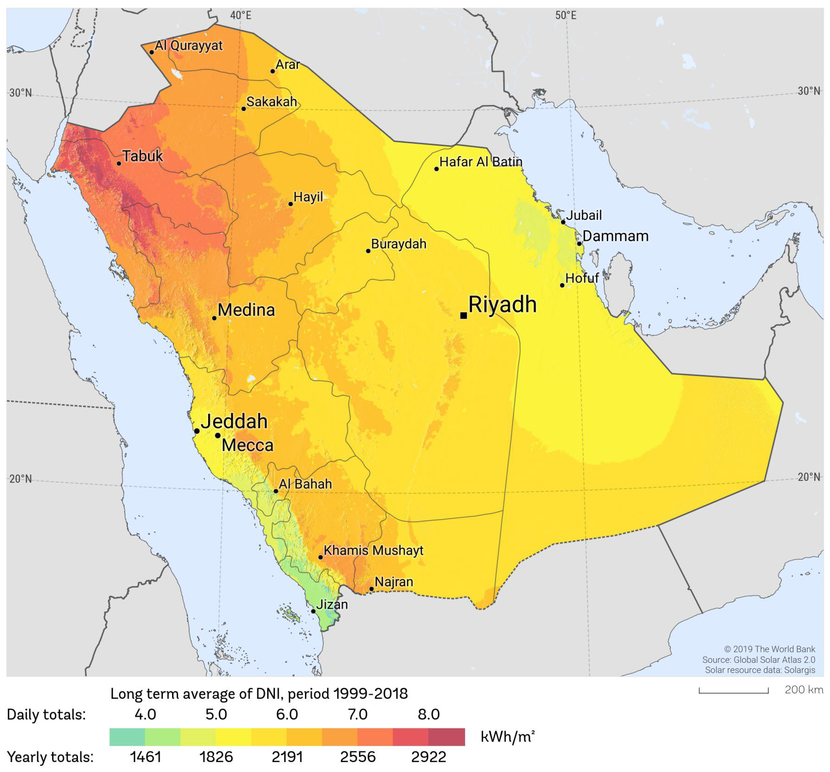
3.1. Geographical Location for the Analysis

Saudi Arabia utilizes more than 3 million barrels per day (mbbl/d) of its daily oil production, that is around 12 mbbl/d, for only domestic power generation [38,39]. Recently, the government of Saudi Arabia launched an ambitious goal, “Vision 2030”, which targets a total instalment of 54 GW of renewables by 2030 [40,41]. CSP accounts for the largest share of renewables’ planned installation of 25 GW while the present installed CSP capacity is just 93 MW [42]. The country has an abundant source of solar radiation; thus, the yearly average DNI value can reach more than 2800 $\mathrm{k}\mathrm{W}\mathrm{h}/{\mathrm{m}}^2/\mathrm{y}\mathrm{e}\mathrm{a}\mathrm{r}$ in the north-western region as seen in Figure 1. Furthermore, it has been suggested in [9] that European nations may potentially engage in the importation of energy produced with CSP from the Middle East and North Africa (MENA) region in the foreseeable future. The case study was conducted in the arid area of the Tabuk region, namely in the city of Duba, Saudi Arabia.

The DNI is the major factor for CSP design and is described as the radiation received at an incident angle from the sun, and it was measured with Pyrheliometers [44]. The highest DNI occurs in these countries because of cloudless weather. The northwest region has one of the highest DNI values in the world at about $9–9.5 \mathrm{k}\mathrm{W}\mathrm{h}/{\mathrm{m}}^2/\mathrm{d}\mathrm{a}\mathrm{y}$ in the Tabuk region particularly [45]. It is worth mentioning that obtaining accurate DNI data is vital because it has a huge impact on the simulation. Many researchers have investigated the DNI accuracy and found that the DNI uncertainty rate could reach up to 15% [44]. Purohit suggested using long term hourly DNI data to simulate the large CSP projects [46]. Additionally, the ambient air temperature has a considerable effect on the thermal performance of the power plant since it impacts the TES and the cooling system of the CSP [47,48]. Site adaptability and land availability are also crucial considerations for any CSP projects, since CSP is less malleable than PV [46].

The high DNI leads to a higher concentration ratio and, ultimately, a higher CF of the power plant, allowing for greater thermal efficiency [49]. For commercial applications, it is recommended that the DNI value falls within the range of 2000 to 2800 kWh/m²/year for CSP installations [50]. Nevertheless, this study specifically targets locations boasting the highest DNI, exceeding 2500 kWh/m². As an exemplification of a very-high DNI location, this study is carried out at the city of Duba, situated in the northwest region of Saudi Arabia, at geographical coordinates 27°44′55.0″ N 35°27′08.6″ E. The region has a significant installation known as the Integration Solar Combined Cycle (ISSC) Duba-1 power plant, which possesses a massive capacity of 550 MW. Notably, within this power plant, 50 MW are generated specifically via the PTC power plant [10]. The meteorological conditions utilized in this study are derived from METEONMRM, a comprehensive dataset comprising over a decade of satellite data. To ensure accuracy and representativeness, an hourly Typical Meteorological Year (TMY) file is employed [51].

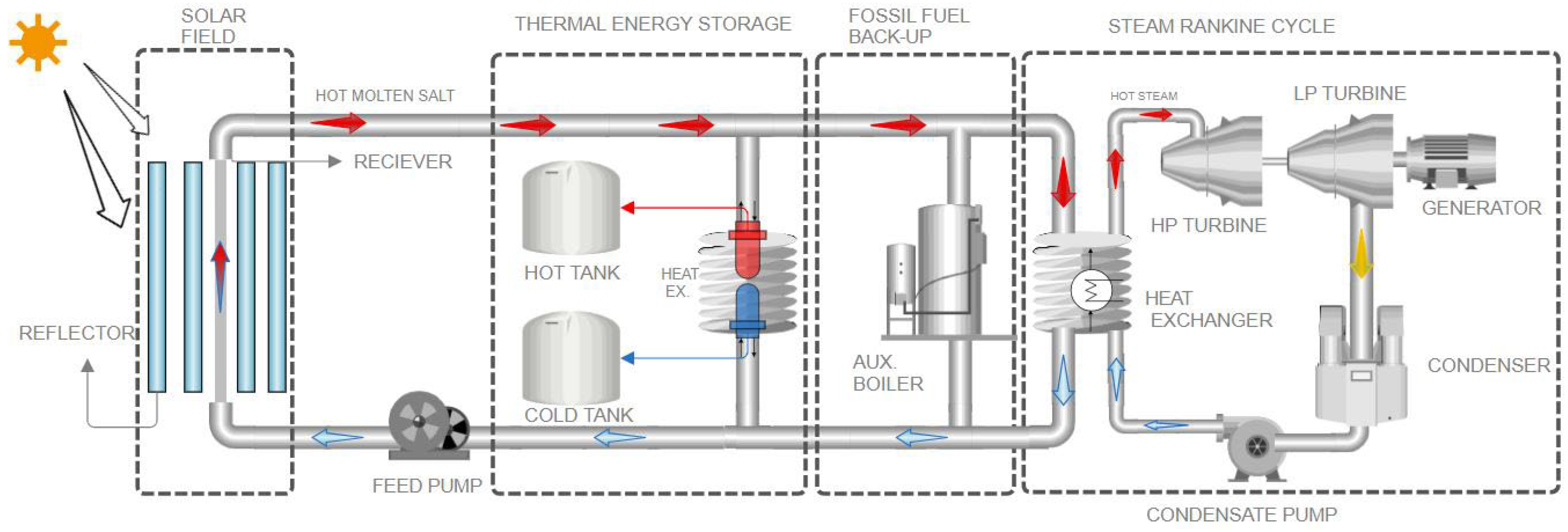
3.2. Off-Design Model Description

The LFR power plant is composed of three primary components: the solar field, which mainly includes the collector and absorber, the thermal energy storage system, and the power block, as illustrated in Figure 2.

For the cooling system, the implementation of a wet cooling system indeed yields a modest enhancement in energy production; however, it concurrently leads to an escalation in water consumption, consequently resulting in increased expenses. [52]. Moreover, the dry (air) cooling may result in higher capital expenditure (CAPEX) and a slight reduction in LFR power output [48]. Nevertheless, it remains a suitable choice for regions with arid climates and ample water resources [52]. Additionally, utilizing a dry cooling system leads to an 80% reduction in the water life cycle consumption [53]. Therefore, dry cooling is used in this analysis for the LFR power plant.

Table 2. Design parameters for all subsections of the LFR power plant used in this analysis (adapted from [23,54,55,56,57]).

Subsection	Parameter	Value
Solar Field	Solar multiple	1–4 (step of 0.1)
	DNI at design	750 $\mathrm{W}/{\mathrm{m}}^2$
	Number of collector modules in a loop	16
	Number of subfield headers	2
Collector	Reflective aperture area	470.3 ${\mathrm{m}}^2$
	Length of collector model	44.8 m
	Length of crossover piping in a loop	15 m
	Piping distance between sequential modules	1 m
	Solar-weighted mirror reflectivity	0.935
	Dirt on mirror derate	0.95
	General optical derate	0.732
Receiver		Schott PTR 70
	Absorber tube inner diameter	0.066 m
	Absorber tube outer diameter	0.07 m
	Glass envelope inner diameter	0.115 m
	Glass envelope outer diameter	0.12 m
Power cycle
	Reference output electric power at design condition	50 ${\mathrm{M}\mathrm{W}}_{\mathrm{e}}$
	Estimated gross-to-net conversion factor	120.7 ${\mathrm{M}\mathrm{W}}_{\mathrm{t}\mathrm{h}}$
	Estimated net output at design	45 ${\mathrm{M}\mathrm{W}}_{\mathrm{e}}$
	Rated cycle conversion efficiency	39.7%
	Boiler operating pressure	100 bar
	Condenser type	Air-cooled
Thermal Storage
	Equivalent full-load thermal storage hours	0–15 (step of 1)
	Height of HTF when tank is full	20 m
	Loss coefficient from the tank	0.4 $\mathrm{W}/{\mathrm{m}}^2-\mathrm{K}$

includes the most important technical parameters for the modeled LFR power plant [23,54,55,56,57].

For the solar field, the compact linear Fresnel reflector (CLFR) represents the cutting-edge technology that has been meticulously engineered by various manufacturers, including Novatec (Karlsruhe, Germany) [58]. It has been observed that this advanced design has the potential to generate a thermal output of approximately 537 $\mathrm{W}/{\mathrm{m}}^2$, as per the specifications of an alternative solar field configuration [30]. The present study involves a comprehensive examination of the Nova-1 collector, a solar energy device manufactured by Novatec [58]. Novatec solar plant, a prominent company, has gained recognition for its utilization of the DSG technique [55]. However, in the past ten years, this technology has been limited in terms of its extensive thermal storage capabilities on a large scale [59]. Nevertheless, the latest version of the Super-Nova collector loop employed by Novatec solar plant incorporates vacuum receiver tubes that are equipped with a secondary reflector [30]. Consequently, this enhancement enables the generation of steam temperatures that reach as high as 520 °C [58,59].

Various types of receivers can be interconnected to create a hybrid-receiver in a solar field, based on the desired output temperature and the objective of cost reduction [60,61]. Montes et al. [60] conducted an analysis on the optimal integration of evacuated and non-evacuated tubes in a hybrid loop, focusing on thermal and economic considerations [60]. It was assumed that non-evacuated tubes have lower CAPEX and operational expenditure (OPEX) costs, and the findings suggest that this configuration could be advantageous in industrial applications, particularly when operating temperatures are not as high as those in power plants. This comprehensive research examines the potential of the Advance receiver (SCHOTT PTR 70) in facilitating the next technological advancement in CSP systems [57]. Specifically, it focuses on the use of MS as a HTF, capable of functioning at temperatures reaching up to 550 °C [57,62].

3.3. Mathematical Description

3.3.1. Simulation Tool

The System Advisor Model (SAM) was developed and released by the National Renewable Energy Laboratory (NREL) of the United States Department of Energy (DOE) [63]. The NREL cooperated with the Novatec Solar manufacturer to examine and validate the DSG-LFR for three different configurations: recirculated baseline, re-circulated with an extra super heater module, and once-through [47]. The model shows a great capability of predicting the annual power plant performance for all three configurations. Moreover, the SAM has remarkable potential in modeling indirect steam generation with thermal energy storage [64]. Additionally, it is considered to have well-developed models for thermal storage and heat losses [65]. The SAM software (2021.12.2) is among a limited number of simulation tools that possess the capability to assess both the overall technical and economic performance, contingent upon the performance of individual subsystems [65]. The temporal resolution of the weather file data, which can be either hourly or sub-hourly, determines the simulation time-step [63]. Finally, the SAM is one of the effective simulation tools which provides techno-economic analysis for large scale plants for not only CSP, but for most renewable-energy technologies [66].

3.3.2. Incident Angel Modifier Method

The concept of the incident angel modifier (IAM) is that the performance of the LFR is expressed in a fourth order polynomial which can calculate the optical efficiency reduction that is caused by the deviation of the incident irradiation angle in both the transversal (T) and longitudinal (L) plane. A case study [15] concluded that the longitudinal incident angle has a greater influence on the LFR than the transversal incident angle. In another study [67], the simple analytical model has been validated against other models and commercial collectors specifications and has been found that the model predicts the IAMs in an accurate way with the deviation up to only 5%. It is worth mentioning that using the factorized IAM will generally predict the annual performance of up to 5% of the real energy production because of the high error when the range of the incident angle is high [68]. Additionally, compared to the heat losses, LFR optical losses have a greater effect on the performance [69].

To begin with, the optical efficiency, ${\eta }_{opt}$, can be calculated by multiplying the losses in the transversal and the longitudinal directions, $K \left({\theta }_L,{\theta }_T\right)$, by the maximum optical efficiency, ${\eta }_{opt,Max}$, as described in Equation (1):

$${\eta }_{opt}\left({\theta }_L,{\theta }_T\right)= K \left({\theta }_L,{\theta }_T\right)·{\eta }_{opt,Max}$$

(1)

where $K \left({\theta }_L,{\theta }_T\right)$ signifies the longitudinal and transversal coefficient of incidence angle modifier. Equation (1) is developed to calculate the IAM coefficient in the longitudinal plane, $K_L\left({\theta }_L\right)$, as is demonstrated in Equation (2) [70]:

$$K_L\left({\theta }_L\right)=cos\left({\theta }_L\right)-\frac{F}{\mathrm{L}}·\sqrt{1+{\left(\frac{w}{4.F}\right)}^2}·sin\left({\theta }_L\right)$$

(2)

where $F$ is the collector focal distance, $\mathrm{L}$ is the collector length, and $w$ is the distance between the centers of the last collectors on the right and on the left.

On the other hand, the total optical losses in the transversal direction, $K_T\left({\theta }_T\right)$, can be calculated with Equation (3) [70]

$$K_T\left({\theta }_T\right)=\left\{\begin{array}{c}cos\left(\frac{{\theta }_T}{2}\right)-\frac{w/4}{F+\sqrt{F^2+({w/4)}^2}} sin\left(\frac{{\theta }_T}{2}\right) {\theta }_T<{\theta }_{T,Crit}\\ [cos\left(\frac{{\theta }_T}{2}\right)-\frac{w/4}{F+\sqrt{F^2+({w/4)}^2}} sin\left(\frac{{\theta }_T}{2}\right)]. \left[\frac{D_w}{W_o}.\frac{cos\left({\theta }_T\right)}{\cos \left(\frac{{\theta }_T+{\phi }_m}{2}\right)}\right] {\theta }_T\ge {\theta }_{T,Crit}\end{array}\right\}$$

(3)

where $D_w$ is the distance between the two collectors’ centers, $W_o$ is the width of one collector, and ${\phi }_m$ is the mean value of the angle ${\phi }_i$ that represents the shading area for different collectors.

Similarly, the SAM deploys a fourth order polynomial in terms of transversal and longitudinal incident angles to predict the optical losses in both planes with both Equations (4) and (5).

$${IAM}_T=C_0+C_1·{\theta }_T+C_2\cdot {\theta }_T^2+C_3\cdot {\theta }_T^3+C_4\cdot {\theta }_T^4$$

(4)

$${IAM}_L=C_0+C_1·{\theta }_L+C_2\cdot {\theta }_L^2+C_3\cdot {\theta }_L^3+C_4\cdot {\theta }_L^4$$

(5)

where ${\theta }_L$ is the longitudinal incident angle, ${\theta }_T$ is the transversal incident angle, and the constants $C_{0-4}$ are numerical quantities as seen in

Table 3. Constants of the transversal and longitudinal incident angle modifier coefficients.

Plane	${\mathit{C}}_0$	${\mathit{C}}_1$	${\mathit{C}}_2$	${\mathit{C}}_3$	${\mathit{C}}_4$
Transverse incident angle modifier	0.9896	0.044	−0.0721	−0.2327	0
Longitudinal incident angle modifier	1.0031	−0.2259	0.5368	−1.6434	0.7222

[27].

By employing the polynomial, which varies in accordance with both angles, at each time step, it can predict effectively, calculate the optical losses, and hence simulate the annual performance of the plant.

3.3.3. Technical Performance Model

First, the economic calculation requires the solar field size and total land area, as the latter comprises the overall site preparation costs, in addition to the SF cost. Importantly, the solar field area is expressed as the solar multiple, which is the ratio of the thermal power provided by the SF, ${\dot{Q}}_{sf}$, under the design condition, ${SM}_{des}$, to the power required by the turbine, ${\dot{Q}}_{Pb}$, as shown in Equation (6) [31]:

$${SM}_{des}={\left.\frac{{\dot{Q}}_{sf}}{{\dot{Q}}_{Pb}}\right|}_{design conditions}$$

(6)

For instance, when the SM is equal to 1, the mirror aperture area can satisfy the power cycle’s thermal design output, i.e., the SF’s thermal output can drive the turbine at its rated capacity.

The optical efficiency, in general, is defined as shown in Equation (7):

$${\eta }_{opt}=\frac{E_{R,thermal}}{{Area}_{Actual Aperture} }$$

(7)

where $E_{R,thermal}$ is the solar field’s received thermal energy. However, the total optical efficiency includes several other efficiencies in the solar field. Therefore, the useful thermal received by the solar field may be described by several critical factors. Thus, the incident thermal heat on the solar field, ${\dot{Q}}_{inc}$, in terms of the IAM can be described as in Equation (8):

$${\dot{Q}}_{inc}={\eta }_0. IAM.A_{SF}. DNI$$

(8)

For the design stage, the IAM estimated to 1 and the optical efficiency is around 0.6 [71]. Subsequently, the thermal power produced by the solar field can be calculated with Equation (9) [27]:

$${\dot{Q}}_{SF}={\dot{Q}}_{inc}-{\dot{Q}}_{loss}-{\dot{Q}}_{pipes}$$

(9)

where ${\dot{Q}}_{loss}$ is the heat losses for the collector and receiver, and ${\dot{Q}}_{pipes}$ is the heat losses in the pipes. The heat losses through the pipes, for a specific absorber type, can be calculated using Equation (10), a third order polynomial [62], as follows:

$${\dot{Q}}_{loss}=a_1{(T_{ave}-T_{amb})}^3+a_2{(T_{ave}-T_{amb})}^2+a_3(T_{ave}-T_{amb})$$

(10)

where the coefficients of PR70 Schott Advanced, developed by NREL, are $a_1=6.779.{10}^{-6}\left[\mathrm{W}/{\mathrm{K}}^3\right],$ $a_2=-0.001823\left[\mathrm{W}/{\mathrm{K}}^2\right],$ and $a_3=0.3207\left[\mathrm{W}/\mathrm{K}\right].$ $T_{ave}$ and $T_{amb}$ are the fluid average temperature in the SF and the ambient air temperature, respectively.

Finally, the total loop conversion efficiency is defined by the aggregate collector efficiency, ${\eta }_{ac}$, and the receiver efficiency, ${\eta }_{ar}$, multiplied by the receiver heat loss efficiency, ${\dot{Q}}_{r,loss}$, as indicated in Equation (11):

$${\eta }_{loop}={\eta }_{ac}. {\eta }_{ar}. {\dot{Q}}_{r,loss}$$

(11)

After accounting for the efficiencies and losses of the SF, the useful thermal energy produced by the field may power the turbine and charge the thermal energy storage.

3.3.4. Thermal Energy Storage System

The main components of the TES subsection are the storage tank, HTF, storage media, heat exchanger, pumps, and the insulation. The TES system is composed of cold and hot unpressurised cylindrical tanks, each equipped with pumps, insulation, and sensors [72]. During this study, the geometry and thermodynamic parameters of the TES system vary.

The size of the TES is indicated in terms of the number of full load hours ($t_{full load}$) and, firstly, the storage volume, $V_{TES}$, can be expressed as in Equation (12):

$$V_{TES}=\frac{C . 1\times e^6. 3600}{{\rho }_{HTF}. c_{HTF}. 1000.{\mu }_{hx}.(\left(T_{sf,out}-T_{hx,hot}\right)-\left(T_{sf,in}-T_{hx,cold}\right))}$$

(12)

where $C$ is the TES thermal capacity, ${\rho }_{HTF}$ is the fluid density, $c_{HTF}$ is the specific heat of the used fluid, ${\mu }_{hx}$ is the heat exchanger derate, $T_{sf}$ is the inlet and outlet solar field temperatures, and $T_{hx,}$ is the hot and cold temperatures of the heat exchanger.

To calculate the thermal capacity of the TES, the efficiency of the TES and design work of the pump at the design conditions is required. It can be described with Equation (13):

$$C=\frac{{\dot{W}}_{des,gross}}{{\eta }_{des}}\times t_{full load}$$

(13)

where ${\dot{W}}_{des,gross}$ is the design gross work of the pump (generally 0.85) [26], and ${\eta }_{des}$ is the thermal efficiency of the TES at the design condition.

Additionally, the diameter of the tank can be determined using Equation (14):

$$D_{tank}=2\times \sqrt{\frac{V_{TES}}{h_{tank}. \pi . N_{pairs }}}$$

(14)

where $h_{tank}$ is the tank height and $N_{pairs }$ is the number of tank pairs. In this analysis, 1 pair of tanks is utilized.

Finally, the TES heat losses, ${hl}_{TES}$, are equivalent to the product of the total interacting cylindrical tank area, number of tank pairs, the temperature difference of the TES, on average, with ambient air, and the heat loss coefficient for the tanks $C_{hl,tank}$, which is indicated in Equation (15):

$${hl}_{TES}=\left( h_{tank} . \pi . D_{tank}+\pi . {\left(\frac{D_{tank}}{2}\right)}^2\right). N_{pairs }. \left(T_{TES,ave}-T_{ambient}\right). C_{hl,tank}$$

(15)

3.3.5. Economic Analysis

The net discounted cost to develop and run a power project divided by the total amount of electricity generated over the project’s lifetime is known as the “LCOE”, which is a measure of comparative power generation costs for different renewable technologies [2]. In addition to the atmospheric and the technical key parameters, the economic parameters such as the LCOE, the NPV, and the payback period are significant in any techno-economic assessment to evaluate the feasibility of the investigated technology.

Table 4. Summary of capital and operational costs and assumptions for important financial assessment.

Cost Type	Description	Value
Direct capital costs	Site improvement	20.00 ${\mathrm{\$}/\mathrm{m}}^2$
	Solar field	150.00 ${\mathrm{\$}/\mathrm{m}}^2$
	HTF system	47.00 ${\mathrm{\$}/\mathrm{m}}^2$
	Thermal energy storage	32.00 ${\mathrm{\$}/\mathrm{k}\mathrm{W}\mathrm{h}}_{\mathrm{t}}$
	Fossil backup	60.00 ${\mathrm{\$}/\mathrm{k}\mathrm{W}}_{\mathrm{e}}$
	Power plant	1100.00 ${\mathrm{\$}/\mathrm{k}\mathrm{W}}_{\mathrm{e}}$
	Balance of plant	340.00 ${\mathrm{\$}/\mathrm{k}\mathrm{W}}_{\mathrm{e}}$
Operation and maintenance costs	Operating cost by capacity	66 $\mathrm{\$}/\mathrm{k}\mathrm{W}.\mathrm{y}$
	Variable operating cost	4 $\mathrm{\$}/\mathrm{M}\mathrm{W}\mathrm{h}$
	Fossil fuel cost	4 $\mathrm{\$}/\mathrm{M}\mathrm{M}\mathrm{B}\mathrm{t}\mathrm{u}$
Financial parameters	Analysis period	25 years
	Inflation rate	2.5%
	Real discount rate	6.4%

indicates CAPEX, OPEX, and major financial parameters for an LFR power plant [56,73,74,75].

The main economic indicator in this analysis is the LCOE which can be calculated with Equation (16) [76]:

$$LCOE=\frac{{\sum }_{n=0}^N{C}_n{(1+r)}^{-n}}{{\sum }_{n=0}^N{E}_n{(1+r)}^{-n}}$$

(16)

where N is the project’s lifetime, n represents the year of the calculation, $C_n$ is total cost for year $n$, $r$ stands for the real discount rate, and $E_n$ is the energy generated in a specific year.

Additionally, the other important consideration in evaluating a CSP power plant’s economic viability is its Net Present Value (NPV), which is shown in Equation (17) [34]:

$$NPV=\sum _{y=1}^N\frac{Annual costs}{{(1+r)}^y}$$

(17)

The Internal Rate of Return (IRR) can be an additional economic indicator for evaluating the project which can be calculated with Equation (18) [3].

$$\sum _{t=0}^n\frac{Revenue-costs}{{(1+IRR)}^{Project Lifetime}}=0$$

(18)

Various mathematical descriptions of all the financial indicators may be calculated depending on the type of investment or the requirement to assess the projects. After demonstration of the techno-economic methodology, the outcomes of the assessment are shown in the results section.

3.3.6. Environmental Analysis

In this section, the most crucial environmental parameters are analyzed, and these are the land use, annual water consumption, and GHG emissions. The solar-only configuration, SF coupled with a large TES, and with/without FF backup system scenarios are examined. All the GHG emission factors are indicated in

Table 5. Estimation of most important environmental impact factors (adapted from [23,53,77]).

Power Plant Subsections	Unit	$\mathbf{GHG} \mathbf{Value} (\mathbf{k}\mathbf{g}.{\mathbf{C}\mathbf{O}}_2.\mathbf{e}\mathbf{q}./\mathbf{U}\mathbf{n}\mathbf{i}\mathbf{t})$
Natural gas combustion	$(\mathrm{k}\mathrm{g}/\mathrm{M}\mathrm{W}\mathrm{h})$	95
Solar field	$({\mathrm{m}}^2/\mathrm{M}\mathrm{W}\mathrm{h})$	${8.4\times 10}^{-7}$
HTF system	$({\mathrm{m}}^2/\mathrm{M}\mathrm{W}\mathrm{h})$	${5.1\times 10}^{-7}$
TES system	$({\mathrm{M}\mathrm{W}\mathrm{h}}_{\mathrm{t}\mathrm{h}}/\mathrm{M}\mathrm{W}\mathrm{h})$	${3.3\times 10}^{-4}$
Power block	$(\mathrm{M}\mathrm{W}/\mathrm{M}\mathrm{W}\mathrm{h})$	${7.8\times 10}^{-4}$

, which includes all the emissions from the subsections of the LFR power plant [23,53,77].

Land usage fluctuates across the assessment as the SM changes, with a single loop aperture necessitating 7524.8 ${\mathrm{m}}^2$, serving as the basis for determining the overall land requirement. Furthermore, to address water usage concerns, a dry condenser is chosen which is suitable for arid regions facing water scarcity. However, the maintenance process involves cleaning collectors, which consume 0.02 ${\mathrm{L}/\mathrm{m}}^2$ of the aperture area and require 120 washes annually [52].

4. Result and Discussion

4.1. Model Validation

The validation process is carried out in two stages. Since this analysis focuses on the molten-salt LFR technology with a large TES, the first validation step is conducted against the Chinese Dacheng Dunhuang power plant data, as indicated in Table 2. This power plant is the only operational facility of its kind globally, utilizing molten salt in both HTF and TES, with a nominal capacity of 50 MW. The power plant was initially put into operation in 2019; therefore, it has only been running for a few years [42]. The simulated model in SAM exhibits a sufficient agreement with the techno-economic performance and the provided data profile, as seen in

Table 6. Validation of the present model against the actual 50 MW LFR power plant in China.

Parameter Type	Solar Field and Performance Parameters	Unit	Dacheng Dunhuang Power Plant	Present Model	Deviation
Major techno-economic parameter	Turbine capacity	$\mathrm{M}\mathrm{W}$	50	50	$-$
	TES capacity	$\mathrm{h}\mathrm{o}\mathrm{u}\mathrm{r}\mathrm{s}$	13	13	$-$
	Solar field aperture area	${\mathrm{m}}^2$	1.27	1.27	$-$
	PPA price in year 1	$\mathrm{¢}/\mathrm{k}\mathrm{W}\mathrm{h}$	17	17	$-$
Actual and simulated annual performance	Total land area	${\mathrm{m}}^2$	3.2	3.18	−1%
	Annual energy generated	$\mathrm{G}\mathrm{W}\mathrm{h}$	214	216	1%
	Capacity factor	$\mathrm{\%}$	$-$	54.8	$-$
	Annual water usage	${\mathrm{m}}^3$	$-$	19,448	$-$
	Net capital costs	$\mathrm{m}\mathrm{i}\mathrm{l}\mathrm{l}\mathrm{i}\mathrm{o}\mathrm{n} \mathrm{\$}$	253	257	1%
	LCOE	$\mathrm{¢}/\mathrm{k}\mathrm{W}\mathrm{h}$	10	9.84	−2%
	Specific cost	$\mathrm{\$}/\mathrm{k}\mathrm{W}$	5064	5135	1%

[78].

The simulated model shows good agreement with the actual power plant. The maximum deviation between both is only 2% for the LCOE. Since the actual power plant lacks some technical data, a further step in the validation is performed against the published data to validate the LFR power plant without a TES system, increasing the confidence in the developed model. The summary of both models’ results is provided in

Table 7. Validation of the present model against the published data of the 50 MW LFR power plant in Spain.

Parameter Type	Solar Field and Performance Parameters	Unit	Spain Model	Present Model	Deviation
Solar field input parameters	Number of loops	$-$	50	50	$-$
	Solar multiple	$-$	1.72	1.72	$-$
	Actual solar field aperture area	${\mathrm{m}}^2$	411,000	411,000	$-$
Published and simulated annual performance	Total solar field area	${\mathrm{m}}^2$	757,000	739,603	−2%
	Solar thermal power	${\mathrm{M}\mathrm{W}}_{\mathrm{t}\mathrm{h}}$	218	207	−5%
	Annual energy generation	$\mathrm{G}\mathrm{W}\mathrm{h}$	102	102	0%
	Capacity factor	$\mathrm{\%}$	23.4%	23.7%	1%
	Annual water usage	${\mathrm{m}}^3$	$-$	288,207	$-$
	LCOE	$\mathrm{¢}/\mathrm{k}\mathrm{W}\mathrm{h}$	13.61	13.22	−3%
	Net capital cost	$\mathrm{m}\mathrm{i}\mathrm{l}\mathrm{l}\mathrm{i}\mathrm{o}\mathrm{n} \mathrm{\$}$	$-$	167	$-$

.

The models demonstrate good agreement, with a maximum variance of 5% for the solar thermal power of the SF. Therefore, the purpose of this study can confidently be completed after establishing the agreement in both validation processes.

4.2. Techno-Economic Performance

Maximizing the AEG depends on factors such as the SF area and the TES’s full load hours, but it is associated with an increase in CAPEX. In this study, a parametric analysis is conducted to find the optimal configuration of the SM (with ranges from 1 to 4) and the TES (with a range of 0 to 18 h) in order to achieve the lowest LCOE. Before beginning the parametric analysis, a preliminary simulation of an LFR power plant without and with a large TES is performed to demonstrate the impact of installing storage on the overall power plant performance.

Table 8. Summary of the important techno-economic parameters for the LFR power plant with and without thermal energy storage.

Parameter	Unit	TES = 0	TES = 18	Change
Annual electricity generated	$\mathrm{G}\mathrm{W}\mathrm{h}$	131	351	169%
Capacity factor	$\mathrm{\%}$	33.2	89.1	168%
Annual water usage	${\mathrm{m}}^3$	11,553	29,143	152%
LCOE	$\mathrm{¢}/\mathrm{k}\mathrm{W}\mathrm{h}$	11.92	9.34	−22%
Net capital cost	$\mathrm{m}\mathrm{i}\mathrm{l}\mathrm{l}\mathrm{i}\mathrm{o}\mathrm{n} \mathrm{\$}$	225	513	128%

summarizes the key techno-economic indicators for the LFR with (maximum range 18 h) and without (zero hours) thermal energy storage.

It is clear from Table 8 that installing huge TES increases the technical performance of the LFR plant by about 170% in the yearly amount of energy; however, it also increases the costs by about 130%. Figure 3 clearly illustrates how the utilization of a large TES significantly increases the monthly energy production.

The large TES can supply at least 17 GWh per month throughout the year, but the LFR plant without storage could never deliver 15 GWh per month, even during the summer when the DNI is at its peak. During the summer months, the massive TES can generate approximately 35 GWh per month, but the power plant without the TES can only supply 1/3 of that amount of energy. Additionally, the electricity production for the system with TES produces electricity in the winter months more than the LFR without storage even during its highest capacity in summer. Clearly, this increase in annual energy output comes at a cost in the SF and TES expenditures.

Both simulated models (with and without TES) have been analyzed and compared technically and economically with published data of two power plants in Spain and Algeria [23,27]. A summary of the comparison is summarized in

Table 9. Comparison between the presented models (with and without thermal energy storage) against two published LFR power plant datasets from Spain and Algeria.

Parameter	Unit	Simulated without Storage	Carolina et al. [27]	Simulated Model with Storage	Mihoub et al. [23]
Location	$-$	Duba Saudi Arabia	Seville Spain	Duba Saudi Arabia	Tamanrasset Algeria
Annual DNI	${\mathrm{W}/\mathrm{m}}^2/\mathrm{y}$	2723	2136	2723	2759
Solar multiple	$-$	1.5	2	3.7	2.8
FFF	$\mathbf{\%}$	$-$	$-$	$-$	0.25
Annual electricity generated	$\mathrm{G}\mathrm{W}\mathrm{h}$	131	110	351	$-$
Capacity factor	$\mathbf{\%}$	0.33	0.25	0.89	0.54
TES capacity	$\mathrm{h}\mathrm{o}\mathrm{u}\mathrm{r}\mathrm{s}$	0	0	18	6
LCOE	$\mathrm{¢}/\mathrm{k}\mathrm{W}\mathrm{h}$	11.92	13.44	9.34	13.82
Total cost	$\mathrm{m}\mathrm{i}\mathrm{l}\mathrm{l}\mathrm{i}\mathrm{o}\mathrm{n} \mathrm{\$}$	225	$-$	512	319
Land use	$\mathrm{a}\mathrm{c}\mathrm{r}\mathrm{e}\mathrm{s}$	170	$-$	417	274
Annual water usage	${\mathrm{m}}^3$	11,553	$-$	29,143	$-$

.

The 50 MW LFR power plants with zero hours TES in Saudi Arabia and Spain produced results that were comparatively similar because the only factor affecting the annual performance is the size of the SF. However, the value of the DNI in Duba is greater than the one in Spain, which contributes to the production of more energy at a lower cost. It is noteworthy to mention that a greater DNI value necessitates a smaller solar field, as the thermal energy generated by the solar field is sufficient to power the turbine at its rated capacity. More annual energy generation results in a higher capacity factor, thus leading to a reduction in the electricity costs. In contrast, the LFR plant located in Algeria operates with an FF backup system but still generates electricity at a mere 54 percent of its rated capacity. In contrast, the Duba plant operates at approximately 89 percent of its capacity, owing to the larger TES size of 18 h in the latter scenario. It is worth noting that this increase in the energy output and the size of the TES necessitates an increase in land use of 417 acres, compared to merely 319 acres for Algeria’s power plant. Moreover, from an economic standpoint, the power plants in Duba incur costs of $512 million, whereas the power plant in Algeria is significantly less expensive, at approximately $319 million. Certainly, all these techno-economic criteria fluctuate based on a variety of factors, including site-specific metrological data and the power plant’s decision-makers’ aims. For this reason, it is imperative that these factors—which are parametrically analyzed in the next section—be examined for a particular geographic region.

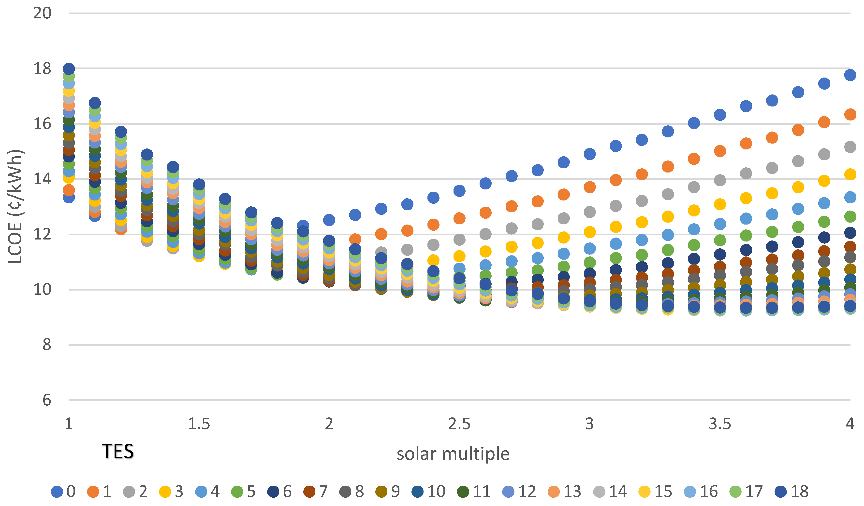
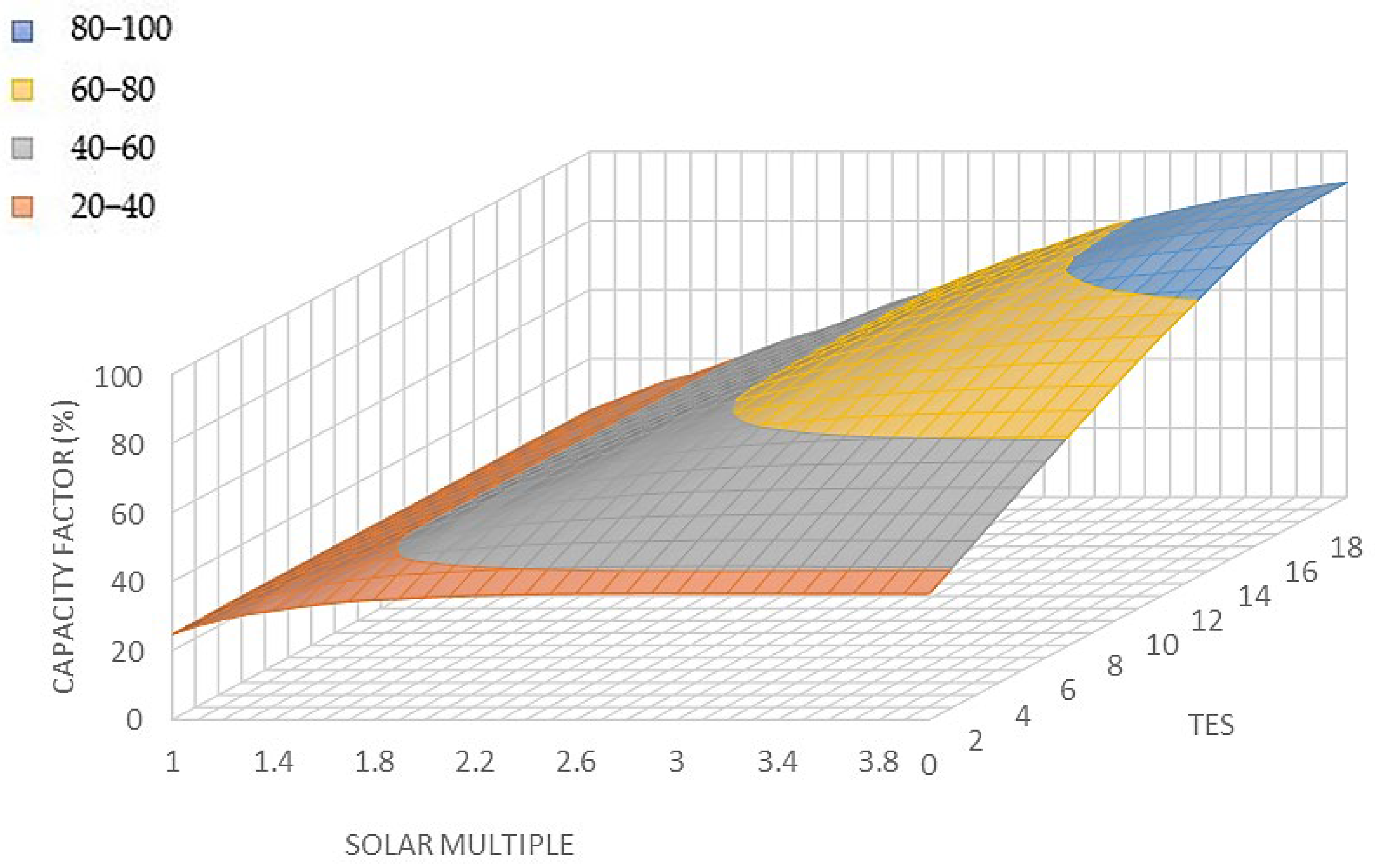
4.3. Thermal Energy Storage and Solar Multiple Optimization

The SAM is utilized to conduct a parametric analysis on the power plant, with a specific emphasis on influential factors such as solar multiple and storage duration. This investigation aims to comprehend the impact of these variables on both the total power generation of the plant and the LCOE [79]. Additionally, a fossil fuel backup system utilizing natural gas is employed to maximize the thermal efficiency and extend the duration of electricity generation. Moreover, oversizing the solar field area and the TES will lead to increasing the CAPEX which also causes an increase in the LCOE, so optimizing the SM is critical to reach competitive costs. The impact of the TES duration (varying from 0 to 18 h with a 1 increment) and the SM (varying from 1 to 4 h with a 0.5 increment) on the LCOE is illustrated in Figure 4. Upon examining the figure, for an SM of 1, the LCOE increases almost linearly with the size of the TES. This is because the SF is incapable of supplying the required amount of thermal energy for storage. Consequently, there is no advantage in expanding the thermal storage. Notably, a solar multiple of one cannot provide the necessary thermal energy for the cycle because of thermal losses in the SF; hence, the SM should often be more than one. When both the solar field area and the storage size are increased, they both achieve their optimum performance; beyond this point, the cost increase will outweigh the thermal advantage of both expansions. Similarly, Figure 5 shows that the lowest LCOE is achieved when the SM is 3.5 and the TES is 15 h, resulting in an LCOE of 9.24 cents/kWh.

Figure 6 clearly shows that oversizing the SM without or with a small storage capacity, as well as oversizing the storage with a small solar field area, results in the maximum electricity cost being more than 15 cents per kWh. For SM values exceeding 2.5 and TES durations exceeding 8 h, the minimum power cost is determined to be below 10 cents per kilowatt-hour. This demonstrates that the LFR’s solar field utilizing molten salt may perform optimally when combined with a massive TES system.

Regarding the electricity generation depicted in Figure 7, expanding the solar field generally enhances the AEG. Notably, for an SM of 1, extending storage duration does not increase the AEG as the solar field only produces thermal energy for the power cycle. However, with a larger solar field, increasing the TES size boosts the energy output until enough thermal energy charges the storage and powers the cycle. Once the solar field is large enough to charge the TES and produce energy, the annual energy remains constant. Oversizing the TES does not affect the annual energy output but increases the costs. It is noteworthy that the optimal SM of 3.5, aimed at achieving the lowest electricity price, generates less energy compared to the SM of 4. Consequently, the decision-maker faces a trade-off between producing higher energy output at a slightly higher electricity price.

Similarly, as depicted in Figure 8, the AEG increases with the expansion of the solar field area until it reaches a plateau. This occurs because the thermal energy becomes adequate to power the turbine at its rated capacity. The impact of the storage size is evident, resulting in an approximate increase of around 10 GWh per year for each additional hour. However, for larger storage sizes (>10 h), while the AEG continues to increase slightly with a larger field area, there is a cost penalty as expenditures surpass the additional electricity production.

In Figure 9, it is evident that enlarging the SF with a small TES size and minimizing the SF alongside low storage duration leads to the lowest AEG. Conversely, larger storage sizes (TES > 14 h) combined with extensive solar field areas (SM > 3) result in the highest electricity production, reaching nearly 400 GWh annually, albeit with higher costs.

Given that the capacity factor is defined as the ratio of the AEG to the maximum potential energy production of the power plant, the optimization results mirror those of annual energy production. As depicted in Figure 10, Figure 11 and Figure 12, increasing the SM and TES elevates the plant’s capacity factor. For smaller solar fields (SM < 2), the CF remains constant or experiences a slight increase with larger storage sizes. Conversely, for SM values exceeding 3, the CF tends to flatten out after the TES exceeds 15 h. This underscores why the optimal TES size is determined to be 15 h concerning the LCOE. Furthermore, the optimal SM is identified as 3.5, resulting in a capacity factor of approximately 86%, while the highest capacity factor of 89% is attained when employing the largest SM and TES configurations.

Lastly, from Figure 12, although the lowest LCOE is found when the SM is 3.5 with the TES of 15 h, implementing a larger solar field (SM = 4) can produce more energy with a comparable price.

Table 10. Summary of the most important techno-economic parameters for all optimum configuration of each thermal energy storage size.

TES (hours)	LCOE (¢/kWh)	Optimal SM (-)	Capacity Factor (%)	AEG (MWh)	Cycle Gross Efficiency (%)	Net Capital Cost ($)	Actual Aperture Area ${(\mathbf{m}}^2)$	Total Water Consumption ${(\mathbf{m}}^3)$
0	11.92	1.5	33%	131,000	16%	225,400,000	428,914	11,553
1	11.36	1.6	37%	145,000	17%	240,308,000	459,013	12,715
2	10.97	1.7	40%	158,000	18%	255,109,000	489,112	13,797
3	10.68	1.9	44%	175,000	19%	276,560,000	541,786	15,155
4	10.44	2	47%	187,000	21%	291,294,000	571,885	16,157
5	10.25	2.2	52%	204,000	22%	314,948,000	632,083	17,588
6	10.07	2.3	55%	214,959	23%	327,442,000	654,658	18,476
7	9.94	2.4	58%	227,000	25%	342,126,000	684,757	19,430
8	9.82	2.5	60%	238,000	25%	356,798,000	714,856	20,328
9	9.69	2.7	65%	256,000	27%	380,502,000	775,054	21,787
10	9.59	2.9	69%	271,836	28%	401,780,000	827,728	23,106
11	9.52	3	72%	283,739	30%	416,234,000	857,827	24,059
12	9.44	3.1	75%	295,802	31%	430,687,000	887,926	25,014
13	9.38	3.2	78%	306,080	32%	442,893,000	910,501	25,834
14	9.30	3.4	83%	325,111	34%	466,335,000	970,699	27,244
15	9.24	3.5	86%	337,018	35%	480,789,000	1,000,798	28,077
16	9.25	3.6	88%	346,011	35%	495,241,000	1,030,898	28,742
17	9.29	3.6	88%	346,822	35%	500,703,000	1,030,898	28,784
18	9.34	3.7	89%	351,378	35%	512,905,000	1,053,472	29,143

presents a comprehensive summary of all optimal SM-TES configurations, along with important distinguishing techno-economic factors.

Analyzing Table 10 reveals a slight variance between the optimal configurations concerning the LCOE, providing decision-makers with flexibility to choose the most suitable configuration based on their objectives. For instance, comparing the optimal configuration of 3.5 SM and 15 h of TES to the largest configuration (SM = 4 and TES = 18 h), the power plant can generate approximately 14 GWh more electricity annually than the lowest LCOE configuration and achieve a 2% higher capacity factor. However, this comes at a higher electricity price, requiring around 53,000 m² more area and roughly $32 million more in net capital cost. Furthermore, a comparison of the optimum configuration with a plant without a TES system emphasizes the importance of utilizing a large TES. The configuration featuring 15 h of thermal storage demonstrates notable advantages, including tripling the annual energy output and achieving a capacity factor 2.6 times higher. Moreover, it reduces electricity prices by approximately 23%. However, it necessitates a solar field area 2.3 times larger, and entails double the capital cost compared to the configuration without a thermal energy storage. These optimal configurations provide leaders with clear guidance for planning the LFR power plant according to their specific requirements and objectives.

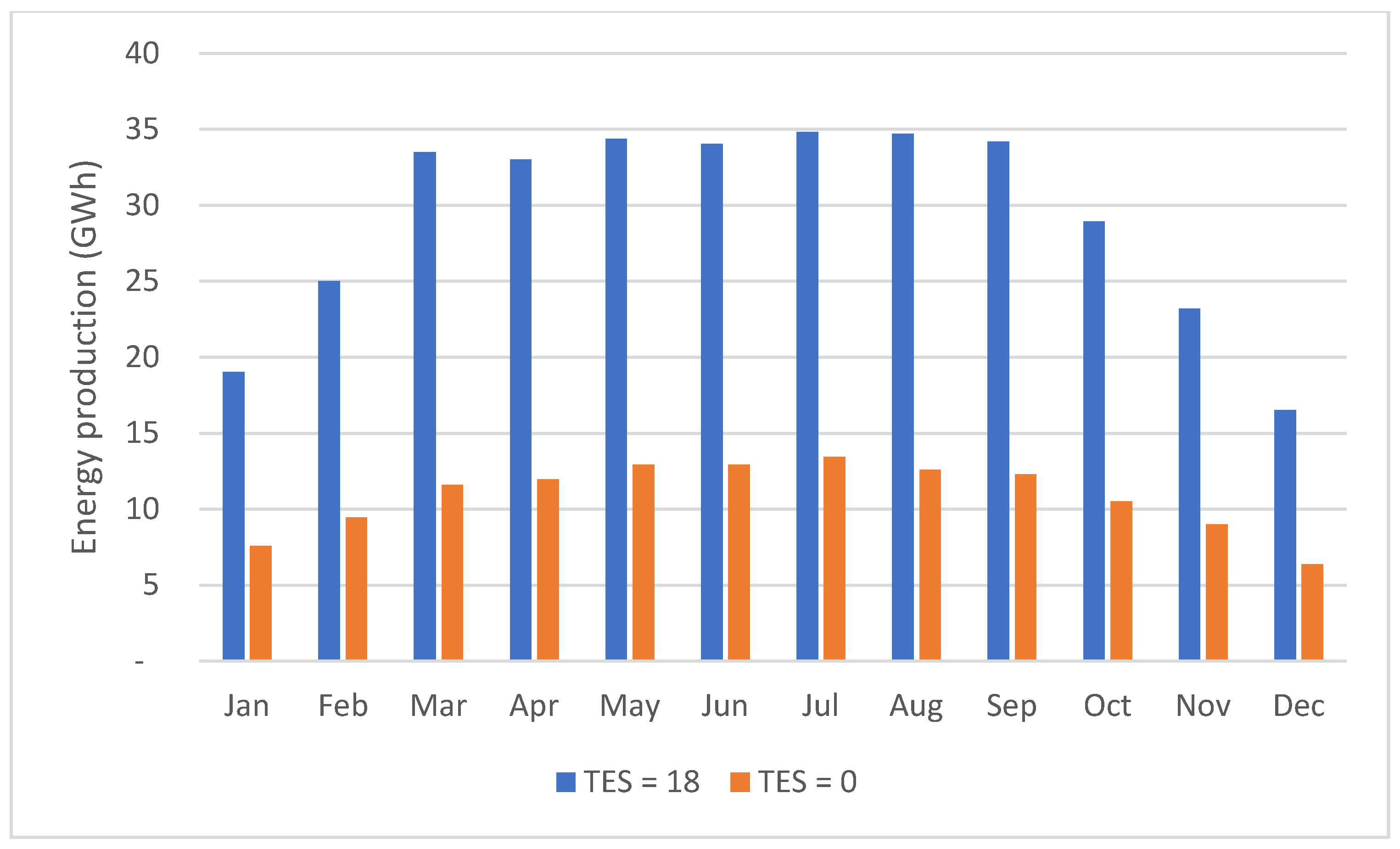
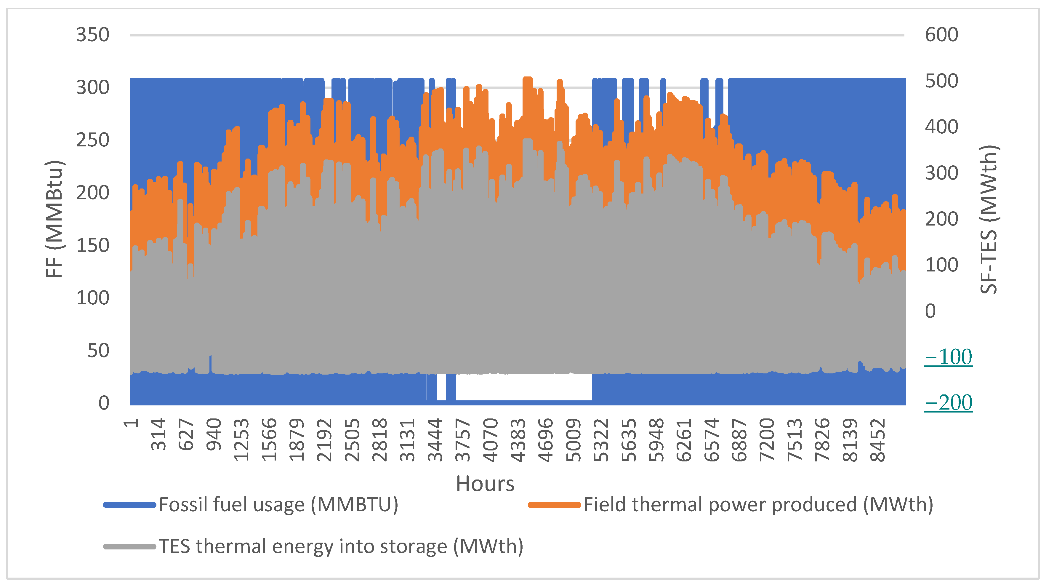
4.4. Power Plant Thermal Performance

Examining the thermal performance of the LFR plant is crucial as it offers valuable insights into the efficiency and effectiveness of the solar field and the storage.

Table 11. Summary of the plant’s thermal performance for all optimum configurations of the solar multiple and thermal energy storage sizes.

TES (Hours)	Optimal SM (-)	Field Thermal Power Incident $\left({\mathbf{M}\mathbf{W}}_{\mathbf{t}\mathbf{h}}\right)$	Field Thermal Power Absorbed $\left({\mathbf{M}\mathbf{W}}_{\mathbf{t}\mathbf{h}}\right)$	Field Thermal Power Produced $\left({\mathbf{M}\mathbf{W}}_{\mathbf{t}\mathbf{h}}\right)$	Thermal Energy into Storage $\left({\mathbf{M}\mathbf{W}}_{\mathbf{t}\mathbf{h}}\right)$	Cycle Thermal Power Input $\left({\mathbf{M}\mathbf{W}}_{\mathbf{t}\mathbf{h}}\right)$
0	1.5	1,167,759	411,316	399,119	-	368,502
1	1.6	1,249,707	439,885	428,465	29,858	406,677
2	1.7	1,331,655	469,007	456,432	55,881	442,106
3	1.9	1,475,064	520,093	504,957	86,961	485,372
4	2	1,557,012	549,152	533,062	114,577	517,978
5	2.2	1,720,908	607,046	589,219	151,963	563,095
6	2.3	1,782,369	628,551	610,894	177,843	592,267
7	2.4	1,864,317	657,592	639,000	205,883	623,154
8	2.5	1,946,265	686,348	667,075	232,655	652,015
9	2.7	2,110,161	743,913	723,234	275,942	698,149
10	2.9	2,253,570	794,860	772,377	315,390	739,872
11	3	2,335,518	823,845	800,400	345,824	770,679
12	3.1	2,417,466	852,658	828,529	376,041	801,614
13	3.2	2,478,927	874,437	849,563	402,399	828,391
14	3.4	2,642,823	928,750	906,123	446,833	872,581
15	3.5	2,724,771	959,870	933,530	473,466	899,168
16	3.6	2,806,719	989,162	961,501	493,987	919,914
17	3.6	2,806,719	989,069	961,508	495,531	921,343
18	3.7	2,868,180	1,011,198	982,127	507,027	931,995

provides insights into the performance of the solar field, including the thermal contribution of the TES system and the quantity of thermal energy supplied to the cycle of all optimum configurations. In all optimum scenarios, the solar field generates around 34% of the total incident thermal power. Subsequently, the quantity of thermal energy provided to the power cycle accounts for approximately 32% of the total thermal energy received by the solar field after accounting for all the thermal losses. It is worth noting that the storage contributes up to 52% of the overall thermal cycle input for the largest optimum design of 18 h. This increases the stability of the power plant to produce energy continuously. In the optimal configuration with a 15 h storage duration and 3.5 solar multiple, the plant is expected to supply approximately 900,000 MW of thermal energy to the cycle, with the TES contributing 52% of the total energy.

Figure 13 clearly depicts the thermal performance of both the solar field and the TES system over the course of a typical day of the year for the optimum configuration. In Figure 13, the solar field initiates the production of thermal energy at 8 in the morning, reaching its peak performance during the afternoon with an output exceeding 300 MW of thermal energy per hour. During this period, the solar field is capable of supplying thermal energy to the cycle and simultaneously charging the storage. As the SF’s thermal performance decreases in the evening, the TES system begins discharging energy to sustain the delivery of energy to the cycle. The significance of the TES system (represented by the purple line) becomes evident when it consistently provides thermal energy to the turbine during the night. This uninterrupted production leads to increased annual electricity generation from the cycle, overcoming the high cost associated with the large TES and consequently lowering the LCOE of the plant.

The combination of 15 h of storage paired with a 3.5 Solar multiple could potentially provide thermal energy to the turbine for a total of over 4000 h throughout the year. To further extend the production time, integrating a backup system could increase energy output, lower the LCOE, and enhance the stability of the power plant.

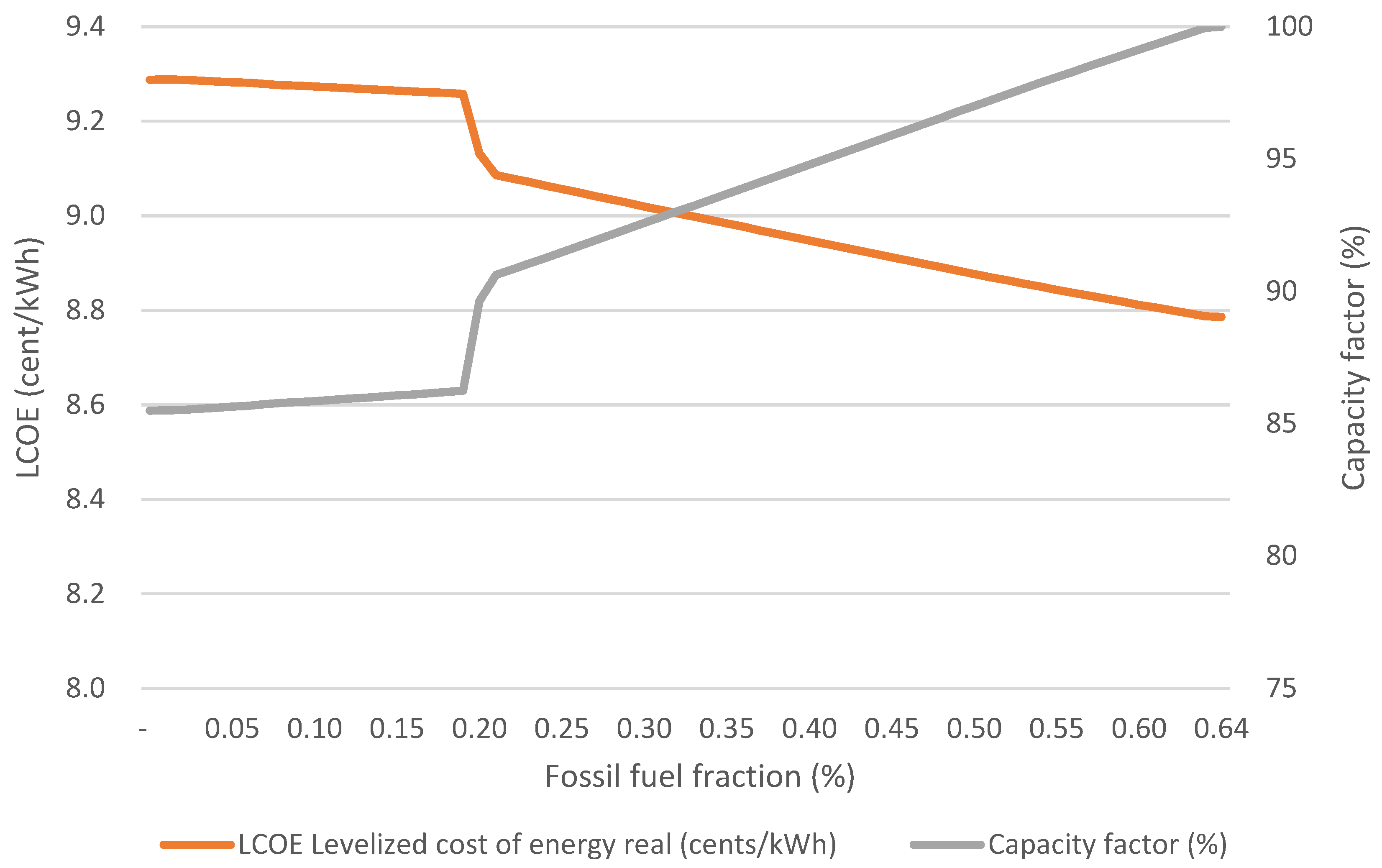
4.5. Backup System Sensitivity Analysis

In this section, the investigation into integrating a fossil fuel backup system with the optimal size of the SF and TES is performed by using the concept of the fossil fuel fraction (FFF). This parameter represents the percentage of energy generated by the boiler (using natural gas) relative to the rated capacity of the turbine. For instance, a FFF of 20% indicates that natural gas powers 20% of the rated turbine capacity. If the solar field and storage can operate the turbine at its rated capacity, there is no requirement to utilize fossil fuels. Moreover, when the FFF is set at, for example, 50%, and the thermal energy from the SF and TES can drive the turbine beyond 50% of its capacity, the backup boiler remains inactive. However, when the temperatures of the HTF in both the solar field and storage drop below the designated low conditions, the fossil fuel backup is engaged to raise their temperatures.

Table 12. The impact of different fossil fuel fractions on the annual techno-economic performance of the 50 MW LFR power plant.

Fossil Fill Fraction	LCOE $(\mathbf{¢}/\mathbf{k}\mathbf{W}\mathbf{h})$	Annual Fuel Energy $\left(\mathbf{G}\mathbf{W}\mathbf{h}\right)$	Annual Energy Generation $\left(\mathbf{G}\mathbf{W}\mathbf{h}\right)$	Capacity Factor $\left(\mathbf{\%}\right)$	Fossil Fuel Usage $\left(\mathbf{M}\mathbf{M}\mathbf{B}\mathbf{t}\mathbf{u}\right)$	Average Gross Cycle Efficiency $\left(\mathit{\%}\right)$
0	9.29	-	337	85.5	-	0.35
0.1	9.27	4	338	85.9	13,107	0.35
0.2	9.13	44	353	89.6	149,647	0.41
0.3	9.02	72	365	92.6	244,049	0.42
0.4	8.95	95	374	94.8	322,236	0.42
0.5	8.88	117	382	97.0	399,308	0.42
0.6	8.81	139	391	99.1	473,122	0.42
0.64	8.79	148	394	100.0	503,429	0.42

provides a sensitivity analysis of the FFF, focusing on the influence of the NG boiler on the annual performance of the LFR power plant.

Table 12 illustrates that the plant achieves its maximum CF of 100% at an FFF of 64%. Increasing the amount of burned NG not only boosts the AEG but also enhances the gross cycle efficiency and reduces the LCOE. Comparing this highest fraction scenario with the LFR system lacking a backup system reveals significant techno-economic disparities. Specifically, an FFF of 64% decreases the LCOE by 5%, increases the AEG by 17%, and improves the cycle efficiency by 20% compared to a system without a backup system. Furthermore, when 64% of FFF is employed, annual fuel usage contributes approximately 44% of the overall annual energy generation. Notably, at a lower FFF of 10%, for example, the backup system only generates 4 GWh annually, indicating that the LFR-TES system alone can meet around 10% of the turbine-rated capacity for almost the entire year.

To clearly depict the findings of the techno-economic influence of the backup system, Figure 14 shows the impact of combining the LFR-TES with a NG backup system on the LCOE and CF. It is evident that when the fossil fuel fraction (FFF) is below 20%, there is minimal alteration in both the LCOE and CF. This observation indicates that the linear Fresnel reflector coupled with a thermal energy storage system can sustain turbine operation for a minimum of 20% annually under these conditions. The influence of the FFF on the overall performance of the plant increases significantly beyond 20 percent, particularly until it reaches 23%. Subsequently, further increments in the FFF demonstrate an almost linear correlation with the increase in the CF and the decrease in the levelized LCOE.

Figure 15 depicts the annual thermal performance of the three primary subsystems of the LFR power plant with an NG backup system. Despite the thermal capabilities of the optimal SF and TES being able to operate the turbine at a capacity factor exceeding 86%, the backup system, with 64% FFF, burns NG for most of the year to enhance the technical performance of the plant. However, during the summer months, the LFR-TES system demonstrates the ability to operate the turbine at its maximum capacity without requiring backup support. This emphasizes the importance of implementing a large TES to generate the highest electricity output, particularly during periods of peak cooling demand in the region. This comes with a penalty of burning approximately 300 MMBtu of natural gas, which is equivalent to more than 500,000 MMBtu annually.

4.6. Environmental Impact

Three different scenarios are compared which represent the optimum solar-only (S1), 3.5 SM with 15 h of TES (S2), and the highest backup fraction (64%) with the optimum configuration of the SF and TES (S3).

Table 13. Summary of the annual environmental impact for the optimum configurations of a 50 MW LFR power plant.

Power Plant Configuration	Water Consumption	Energy Generation	Solar Field	HTF System	TES System	Power Block	Backup System	Total GHG Emissions
	${\mathbf{m}}^3$	$\mathbf{G}\mathbf{W}\mathbf{h}$	$\mathbf{k}\mathbf{g}.{\mathbf{C}\mathbf{O}}_2.\mathbf{e}\mathbf{q}.$				$\mathbf{T}\mathbf{o}\mathbf{n}\mathbf{n}\mathbf{e}.{\mathbf{C}\mathbf{O}}_2.\mathbf{e}\mathbf{q}.$
S1	11,553	131	0.36	0.2	-	0.04	0	0.0006
S2	28,077	337	0.84	0.5	0.156	0.04	0	0.16
S3	31,791	394	0.84	0.5	0.156	0.04	14,027	14,185

presents a comprehensive summary of the annual environmental impact associated with the optimum configurations of a 50 MW LFR power plant. It outlines various parameters such as water consumption, energy generation, and greenhouse gas (GHG) emissions across different components of the power plant configuration.

In terms of water consumption, it is evident that there is a significant disparity among the configurations. S1, with the lowest water consumption at 11,553 ${\mathrm{m}}^3$, contrasts sharply with S3, which consumes substantially more water at 31,791 ${\mathrm{m}}^3$. This discrepancy depends heavily on the amount of generated energy, and this underscores the importance of water management strategies in the design and operation of LFR power plants.

Regarding the land requirements and energy generation, there is a clear progression from S1 to S3, with S3 generating the highest energy output at 394 GWh annually. This increase in energy generation corresponds with the inclusion of various components such as the solar field, TES system, and power block across the configurations. The solar-only scenario requires only 0.6 ${\mathrm{k}\mathrm{m}}^2$ while generating 131 $\mathrm{G}\mathrm{W}\mathrm{h}$. Alternatively, S2 and S3 necessitate 1.6 ${\mathrm{k}\mathrm{m}}^2$ of land for the generation of 337 GWh and 394 GWh, respectively. When comparing S2 and S3, which have identical SM and TES dimensions, the FF backup contributes to an approximate 17% increase in AEG and 13% increase in water usage.

The environmental impact is further delineated through the assessment of GHG emissions, expressed in $\mathrm{T}\mathrm{o}\mathrm{n}\mathrm{n}\mathrm{e}.{\mathrm{C}\mathrm{O}}_2.\mathrm{e}\mathrm{q}$. Notably, S3 exhibits the highest GHG emissions at 14,185 $\mathrm{T}\mathrm{o}\mathrm{n}\mathrm{n}\mathrm{e}.{\mathrm{C}\mathrm{O}}_2.\mathrm{e}\mathrm{q}.$, primarily attributed to the inclusion of a backup system burning natural gas. This highlights the trade-off between energy production and environmental impact, with higher energy generation often accompanied by increased emissions.

Overall, the table provides valuable insights into the environmental implications of different configurations of LFR power plants. Significantly, the NG backup system substantially increases greenhouse gas emissions compared to the minimal 0.16 T$\mathrm{o}\mathrm{n}\mathrm{n}\mathrm{e} {\mathrm{C}\mathrm{O}}_2.\mathrm{e}\mathrm{q}.$ annually associated with the LFR-TES system, offering limited advantages in return. Although the technical advancement for the LFR plant by utilizing the NG backup system is marginal, the principal objective of this analysis is to decrease the LCOE. However, despite this, the integration of the FF backup only results in a 5 percent reduction in costs and a substantial increase in emissions.

5. Conclusions

This study has assessed the deployment of a large LFR plant coupled with a TES system and fossil fuel backup at a high-DNI location in Duba, Saudi Arabia. The optimization results demonstrate that increasing the size of the TES up to 15 h leads to a decrease in the levelized cost of electricity (LCOE) to 8.79 ¢/kWh with a 100% capacity factor. This is achieved with a solar multiple (SM) of 3.5, 15 full load hours of thermal energy storage, and a fossil fuel fraction of 64% of the 50 MW turbine capacity, albeit with increased GHG emissions (~14,000 tCO₂.eq. annually).

Additionally, the study shows that eliminating the natural gas backup results in a slightly higher LCOE of 9.24 ¢/kWh, while a solar-only scenario yields the highest LCOE, i.e., 12 ¢/kWh. The optimization results indicate that molten salt (Hitec Solar Salt), with a fluid output temperature of up to 545 °C, possesses sufficient thermal capacity to be used in combination with a larger TES system, similar to the PTC and SPT technologies [80]. The parametric study results in a 40% decrease in the LCOE, a 300% increase in the AEG, and a 70% increase in the CF when using a 100% renewable energy system.

The findings indicate that increasing the size of the SM and the TES can result in greater energy output. However, this also leads to a higher LCOE, mostly due to the increased CAPEX and OPEX. It is crucial to acknowledge that every geographical area has distinct optimal arrangements of SM-TES sizes. A total of 589 different configurations have been examined in the present study to assist decision makers in selecting the most optimal combination that aligns with their primary goals. This study can provide useful information to policy makers, investors, and other stakeholders related to the costs and performance of the LFR technology. Further, the methods developed and utilized herein can be implemented in other regions with different weather data.

References

1. Dieckmann, S.; Dersch, J.; Giuliano, S.; Puppe, M.; Lüpfert, E.; Hennecke, K.; Pitz-Paal, R.; Taylor, M.; Ralon, P. LCOE reduction potential of parabolic trough and solar tower CSP technology until 2025. AIP Conf. Proc. 2017, 1850, 160004. [Google Scholar]
2. Yao, Y.; Xu, J.H.; Sun, D.Q. Untangling global levelised cost of electricity based on multi-factor learning curve for renewable energy: Wind, solar, geothermal, hydropower and bioenergy. J. Clean. Prod. 2021, 285, 124827. [Google Scholar] [CrossRef]
3. Musi, R.; Grange, B.; Sgouridis, S.; Guedez, R.; Armstrong, P.; Slocum, A.; Calvet, N. Techno-economic analysis of concentrated solar power plants in terms of levelized cost of electricity. AIP Conf. Proc. 2017, 1850, 160018. [Google Scholar]
4. Aly, A.; Bernardos, A.; Fernandez-Peruchena, C.M.; Jensen, S.S.; Pedersen, A.B. Is Concentrated Solar Power (CSP) a feasible option for Sub-Saharan Africa?: Investigating the techno-economic feasibility of CSP in Tanzania. Renew. Energy 2019, 135, 1224–1240. [Google Scholar] [CrossRef]
5. International Renewable Energy Agency. Renewable Power Generation Costs in 2020; International Renewable Energy Agency: Masdar City, United Arab Emirates, 2020. [Google Scholar]
6. British Petroleum. bp Energy Outlook 2023 Edition 2023 Explores the Key Trends and Uncertainties; BP p.l.c.: London, UK, 2023; pp. 1–53. [Google Scholar]
7. Palacios, A.; Barreneche, C.; Navarro, M.E.; Ding, Y. Thermal energy storage technologies for concentrated solar power—A review from a materials perspective. Renew. Energy 2020, 156, 1244–1265. [Google Scholar] [CrossRef]
8. Balghouthi, M.; Trabelsi, S.E.; Amara, M.B.; Bel, A.; Ali, H. Potential of concentrating solar power (CSP) technology in Tunisia and the possibility of interconnection with Europe. Renew. Sustain. Energy Rev. 2016, 56, 1227–1248. [Google Scholar] [CrossRef]
9. Desai, N.B.; Bandyopadhyay, S. Line-focusing concentrating solar collector-based power plants: A review. Clean Technol. Environ. Policy 2017, 19, 9–35. [Google Scholar] [CrossRef]
10. Kassem, A.; Al-Haddad, K.; Komljenovic, D. Concentrated solar thermal power in Saudi Arabia: Definition and simulation of alternative scenarios. Renew. Sustain. Energy Rev. 2017, 80, 75–91. [Google Scholar] [CrossRef]
11. Mills, D.R.; Morrison, G.L. Compact linear fresnel reflector solar thermal powerplants. Sol. Energy 2000, 68, 263–283. [Google Scholar] [CrossRef]
12. Boito, P.; Grena, R. Optimization of the geometry of Fresnel linear collectors. Sol. Energy 2016, 135, 479–486. [Google Scholar] [CrossRef]
13. Abbas, R.; Muñoz-Antón, J.; Valdés, M.; Martínez-Val, J.M. High concentration linear Fresnel reflectors. Energy Convers. Manag. 2013, 72, 60–68. [Google Scholar] [CrossRef]
14. Ladkany, S.; Culbreth, W.; Loyd, N. Molten Salts and Applications III: Worldwide Molten Salt Technology Developments in Energy Production and Storage. J. Energy Power Eng. 2018, 12, 533–544. [Google Scholar]
15. Arias, I.; Cardemil, J.; Zarza, E.; Valenzuela, L.; Escobar, R. Latest developments, assessments and research trends for next generation of concentrated solar power plants using liquid heat transfer fluids. Renew. Sustain. Energy Rev. 2022, 168, 112844. [Google Scholar] [CrossRef]
16. Bellos, E.; Mathioulakis, E.; Tzivanidis, C.; Belessiotis, V.; Antonopoulos, K.A. Experimental and numerical investigation of a linear Fresnel solar collector with flat plate receiver. Energy Convers. Manag. 2016, 130, 44–59. [Google Scholar] [CrossRef]
17. Aljudaya, A.; Ingham, D.; Ma, L.; Hughes, K.; Pourkashanian, M. A Comparative Study of the Techno-Economic Performance of the Linear Fresnel Reflector Using Direct and Indirect Steam Generation: A Case Study under High Direct Normal Irradiance. Int. J. Energy Power Eng. 2023, 17, 255–261. [Google Scholar]
18. Ibrahim, A.; Peng, H.; Riaz, A.; Basit, M.A.; Rashid, U.; Basit, A. Molten salts in the light of corrosion mitigation strategies and embedded with nanoparticles to enhance the thermophysical properties for CSP plants. Sol. Energy Mater. Sol. Cells 2021, 219, 110768. [Google Scholar] [CrossRef]
19. Pan, C.A.; Ferruzza, D.; Guédez, R.; Dinter, F.; Laumert, B.; Haglind, F. Identification of optimum molten salts for use as heat transfer fluids in parabolic trough CSP plants. A techno-economic comparative optimization. AIP Conf. Proc. 2018, 2033, 030012. [Google Scholar]
20. Fernández, A.G.; Cortes, M.; Fuentealba, E.; Pérez, F.J. Corrosion properties of a ternary nitrate/nitrite molten salt inconcentrated solar technology. Renew. Energy 2015, 80, 177–183. [Google Scholar] [CrossRef]
21. Vignarooban, K.; Xu, X.; Arvay, A.; Hsu, K.; Kannan, A.M. Heat transfer fluids for concentrating solar power systems—A review. Appl. Energy 2015, 146, 383–396. [Google Scholar] [CrossRef]
22. Hinkley, J.T.; Hayward, J.A.; Curtin, B.; Wonhas, A.; Boyd, R.; Grima, C.; Tadros, A.; Hall, R.; Naicker, K. An analysis of the costs and opportunities for concentrating solar power in Australia. Renew. Energy 2013, 57, 653–661. [Google Scholar] [CrossRef]
23. Mihoub, S. Design, economic, and environmental assessments of linear Fresnel solar power plants. Environ. Prog. Sustain. Energy 2020, 39, 1–16. [Google Scholar] [CrossRef]
24. Abbas, R.; Montes, M.J.; Piera, M.; Martínez-Val, J.M. Solar radiation concentration features in Linear Fresnel Reflector arrays. Energy Convers. Manag. 2012, 54, 133–144. [Google Scholar] [CrossRef]
25. Santos, J.J.C.S.; Palacio, J.C.E.; Reyes, A.M.M.; Carvalho, M.; Freire, A.J.R.; Barone, M.A. Concentrating Solar Power. Adv. Renew. Energies Power Technol. 2018, 1, 373–402. [Google Scholar]
26. Morin, G.; Dersch, J.; Platzer, W.; Eck, M.; Häberle, A. Comparison of Linear Fresnel and Parabolic Trough Collector power plants. Sol. Energy 2012, 86, 1–12. [Google Scholar] [CrossRef]
27. Marugán-Cruz, C.; Serrano, D.; Gómez-Hernández, J.; Sánchez-Delgado, S. Solar multiple optimization of a DSG linear Fresnel power plant. Energy Convers. Manag. 2019, 184, 571–580. [Google Scholar] [CrossRef]
28. U.S. Department of Energy NREL—National Renewable Energy Laboratory. 2014. Available online: http://www.nrel.gov/ (accessed on 3 February 2020).
29. Bhandari, B.; Lee, K.T.; Lee, G.Y.; Cho, Y.M.; Ahn, S.H. Optimization of hybrid renewable energy power systems: A review. Int. J. Precis. Eng. Manuf. Green Technol. 2015, 2, 99–112. [Google Scholar] [CrossRef]
30. Hakkarainen, E.; Kannari, L. Dynamic Modelling of Concentrated Solar Field for Thermal Energy Storage Integration. In Proceedings of the 9th International Renewable Energy Storage Conference (IRES 2015), Dusseldorf, Germany, 9–11 March 2015. [Google Scholar]
31. Montes, M.J.J.; Abánades, A.; Martínez-Val, J.M.M.; Valdés, M. Solar multiple optimization for a solar-only thermal power plant, using oil as heat transfer fluid in the parabolic trough collectors. Sol. Energy 2009, 83, 2165–2176. [Google Scholar] [CrossRef]
32. Sultan, A.J.; Hughes, K.J.; Ingham, D.B.; Ma, L.; Pourkashanian, M. Techno-economic competitiveness of 50 MW concentrating solar power plants for electricity generation under Kuwait climatic conditions. Renew. Sustain. Energy Rev. 2020, 134, 110342. [Google Scholar] [CrossRef]
33. Alfailakawi, M.S.; Michailos, S.; Ingham, D.B.; Hughes, K.J.; Ma, L.; Pourkashanian, M. Multi-temporal resolution aerosols impacted techno-economic assessment of concentrated solar power in arid regions: Case study of solar power tower in Kuwait. Sustain. Energy Technol. Assess. 2022, 52, 102324. [Google Scholar] [CrossRef]
34. Kumar, S.; Agarwal, A.; Kumar, A. Financial viability assessment of concentrated solar power technologies under Indian climatic conditions. Sustain. Energy Technol. Assess. 2020, 43, 100928. [Google Scholar] [CrossRef]
35. Xu, X.; Vignarooban, K.; Xu, B.; Hsu, K.; Kannan, A.M. Prospects and problems of concentrating solar power technologies for power generation in the desert regions. Renew. Sustain. Energy Rev. 2016, 53, 1106–1131. [Google Scholar] [CrossRef]
36. AREVA. AREVA Delivers the Most Cost-Effective and Land-Efficient CSP Technology-in the Most Environmentally Responsible and Water-Conservative Manner; AREVA: Paris, France, 2011. [Google Scholar]
37. Cspfocus. Project Database. 2017. Available online: http://www.cspfocus.cn/en/study/detail_94.htm (accessed on 12 February 2020).
38. Xu, Y.; Pei, J.; Yuan, J.; Zhao, G. Concentrated solar power: Technology, economy analysis, and policy implications in China. Environ. Sci. Pollut. Res. 2022, 29, 1324–1337. [Google Scholar] [CrossRef]
39. Fernández, A.G.; Gomez-Vidal, J.; Oró, E.; Kruizenga, A.; Solé, A.; Cabeza, L.F. Mainstreaming commercial CSP systems: A technology review. Renew. Energy 2019, 140, 152–176. [Google Scholar] [CrossRef]
40. Hafez, A.A.; Nassar, Y.F.; Hammdan, M.I.; Alsadi, S.Y. Technical and Economic Feasibility of Utility-Scale Solar Energy Conversion Systems in Saudi Arabia. Iran. J. Sci. Technol. Trans. Electr. Eng. 2020, 44, 213–225. [Google Scholar] [CrossRef]
41. Amran, Y.H.A.; Amran, Y.H.M.; Alyousef, R.; Alabduljabbar, H. Renewable and sustainable energy production in Saudi Arabia according to Saudi Vision 2030; Current status and future prospects. J. Clean. Prod. 2020, 247, 119602. [Google Scholar] [CrossRef]
42. Alami, A.H.; Olabi, A.; Mdallal, A.; Rezk, A.; Radwan, A.; Rahman, S.M.A.; Shah, S.K.; Abdelkareem, M.A. Concentrating solar power (CSP) technologies: Status and analysis. Int. J. Thermofluids 2023, 18, 100340. [Google Scholar] [CrossRef]
43. SOLARGIS. Global Solar Atlas 2.0; The World Bank: Washington, DC, USA, 2019. [Google Scholar]
44. AlYahya, S.; Irfan, M.A. Analysis from the new solar radiation Atlas for Saudi Arabia. Sol. Energy 2016, 130, 116–127. [Google Scholar] [CrossRef]
45. Alyahya, S.; Irfan, M.A. The techno-economic potential of Saudi Arabia’s solar industry. Renew. Sustain. Energy Rev. 2016, 55, 697–702. [Google Scholar] [CrossRef]
46. Purohit, I.; Purohit, P.; Shekhar, S. Evaluating the potential of concentrating solar power generation in Northwestern India. Energy Policy 2013, 62, 157–175. [Google Scholar] [CrossRef]
47. Wagner, M.J.; Zhu, G. A direct-steam linear fresnel performance model for NREL’s system advisor model. In Proceedings of the ASME 2012 6th International Conference on Energy Sustainability collocated with the ASME 2012 10th International Conference on Fuel Cell Science, Engineering and Technology, San Diego, CA, USA, 23–26 July 2012; pp. 459–468. [Google Scholar]
48. Yilmazoglu, M.Z. Effects of the selection of heat transfer fluid and condenser type on the performance of a solar thermal power plant with technoeconomic approach. Energy Convers. Manag. 2016, 111, 271–278. [Google Scholar] [CrossRef]
49. Kuravi, S.; Trahan, J.; Goswami, D.Y.; Rahman, M.M.; Stefanakos, E.K. Thermal energy storage technologies and systems for concentrating solar power plants. Prog. Energy Combust. Sci. 2013, 39, 285–319. [Google Scholar] [CrossRef]
50. Islam, M.T.; Huda, N.; Abdullah, A.B.; Saidur, R. A comprehensive review of state-of-the-art concentrating solar power (CSP) technologies: Current status and research trends. Renew. Sustain. Energy Rev. 2018, 91, 987–1018. [Google Scholar] [CrossRef]
51. METEONORM. Weather Data for Any Location on Earth. Available online: https://meteonorm.com/ (accessed on 25 September 2022).
52. Soomro, M.I.; Mengal, A.; Memon, Y.A.; Khan, M.W.A.; Shafiq, Q.N.; Mirjat, N.H. Performance and economic analysis of concentrated solar power generation for Pakistan. Processes 2019, 7, 575. [Google Scholar] [CrossRef]
53. Klein, S.J.W.; Rubin, E.S. Life cycle assessment of greenhouse gas emissions, water and land use for concentrated solar power plants with different energy backup systems. Energy Policy 2013, 63, 935–950. [Google Scholar] [CrossRef]
54. Bishoyi, D.; Sudhakar, K. Modeling and performance simulation of 100 MW LFR based solar thermal power plant in Udaipur India. Resour. Technol. 2017, 3, 365–377. [Google Scholar] [CrossRef]
55. Enriquez, L.C.; Antón, J.M.; Martínez-Val, J.M. Peñalosa SolarPaces 2013: Innovations on direct steam generation in linear fresnel collectors. In Proceedings of the SolarPACES 2013, Las Vegas, NV, USA, 17–20 September 2013. [Google Scholar]
56. Kurup, P.; Turchi, C.S. Parabolic Trough Collector Cost Update for the System Advisor Model (SAM); Technical Report NREL/TP-6A20-65228; National Renewable Energy Laboratory: Golden, CO, USA, 2015; pp. 1–40. [Google Scholar]
57. SCHOTT. SCHOTT PTR 70 Receiver; SCHOTT: Mainz, Germany, 1992. [Google Scholar]
58. Ghodbane, M.; Boumeddane, B.; Said, Z.; Bellos, E. A numerical simulation of a linear Fresnel solar reflector directed to produce steam for the power plant. J. Clean. Prod. 2019, 231, 494–508. [Google Scholar] [CrossRef]
59. Zhu, G.; Wendelin, T.; Wagner, M.J.; Kutscher, C. History, current state, and future of linear Fresnel concentrating solar collectors. Sol. Energy 2014, 103, 639–652. [Google Scholar] [CrossRef]
60. Montes, M.J.; Abbas, R.; Muñoz, M.; Muñoz-Antón, J.; Martínez-Val, J.M. Advances in the linear Fresnel single-tube receivers: Hybrid loops with non-evacuated and evacuated receivers. Energy Convers. Manag. 2017, 149, 318–333. [Google Scholar] [CrossRef]
61. Barbero, R.; Rovira, A.; Montes, M.J.; Val, J.M.M. A new approach for the prediction of thermal efficiency in solar receivers. Energy Convers. Manag. 2016, 123, 498–511. [Google Scholar] [CrossRef]
62. Burkholder, F.; Kutscher, C. Heat Loss Testing of Schott’s 2008 PTR70 Parabolic trough Receiver; Technical report NREL/TP-550-45633; National Renewable Energy Laboratory: Golden, CO, USA, 2009. [Google Scholar]
63. Blair, N.; DiOrio, N.; Freeman, J.; Gilman, P.; Janzou, S.; Neises, T.; Wagner, M. System Advisor Model (SAM) General Description; No. NREL/TP-6A20-70414; National Renewable Energy Laboratory: Golden, CO, USA, 2018. [Google Scholar]
64. Ezeanya, E.K.; Massiha, G.H.; Simon, W.E.; Raush, J.R.; Chambers, T.L. System advisor model (SAM) simulation modelling of a concentrating solar thermal power plant with comparison to actual performance data. Cogent Eng. 2018, 5, 1524051. [Google Scholar] [CrossRef]
65. Ho, C.K. Software and Codes for Analysis of Concentrating Solar Power Technologies; Contract; Sandia National Laboratories (SNL): Albuquerque, NM, USA; Livermore, CA, USA, 2008. [Google Scholar]
66. Tozzi, P.; Jo, J.H. A comparative analysis of renewable energy simulation tools: Performance simulation model vs. system optimization. Renew. Sustain. Energy Rev. 2017, 80, 390–398. [Google Scholar] [CrossRef]
67. Bellos, E.; Tzivanidis, C. Development of analytical expressions for the incident angle modifiers of a linear Fresnel reflector. Sol. Energy 2018, 173, 769–779. [Google Scholar] [CrossRef]
68. Hertel, J.D.; Martinez-Moll, V.; Pujol-Nadal, R. Estimation of the influence of different incidence angle modifier models on the biaxial factorization approach. Energy Convers. Manag. 2015, 106, 249–259. [Google Scholar] [CrossRef]
69. Montes, M.J.; Rubbia, C.; Abbas, R.; Martínez-Val, J.M. A comparative analysis of configurations of linear fresnel collectors for concentrating solar power. Energy 2014, 73, 192–203. [Google Scholar] [CrossRef]
70. Said, Z.; Ghodbane, M.; Hachicha, A.A.; Boumeddane, B. Optical performance assessment of a small experimental prototype of linear Fresnel reflector. Case Stud. Therm. Eng. 2019, 16, 100541. [Google Scholar] [CrossRef]
71. Rungasamy, A.E.; Craig, K.J.; Meyer, J.P. Comparative study of the optical and economic performance of etendue-conserving compact linear Fresnel reflector concepts. Sol. Energy 2019, 181, 95–107. [Google Scholar] [CrossRef]
72. Bauer, T.; Odenthal, C.; Bonk, A. Molten Salt Storage for Power Generation. Chem. Ing. Tech. 2021, 93, 534–546. [Google Scholar] [CrossRef]
73. Alshammari, Y.M. Scenario analysis for energy transition in the chemical industry: An industrial case study in Saudi Arabia. Energy Policy 2021, 150, 112128. [Google Scholar] [CrossRef]
74. Craig, T. Parabolic Trough Reference Plant for Cost Modeling with the Solar Advisor Model (SAM); NREL/TP-550-47605; National Renewable Energy Laboratory: Golden, CO, USA, 2010; p. 112. [Google Scholar]
75. Poghosyan, V.; Hassan, M.I. Techno-economic assessment of substituting natural gas based heater with thermal energy storage system in parabolic trough concentrated solar power plant. Renew. Energy 2015, 75, 152–164. [Google Scholar] [CrossRef]
76. Zhao, Z.Y.; Chen, Y.L.; Thomson, J.D. Levelized cost of energy modeling for concentrated solar power projects: A China study. Energy 2017, 120, 117–127. [Google Scholar] [CrossRef]
77. Whitaker, M.B.; Heath, G.A.; Burkhardt, J.J.; Turchi, C.S. Life cycle assessment of a power tower concentrating solar plant and the impacts of key design alternatives. Environ. Sci. Technol. 2013, 47, 5896–5903. [Google Scholar] [CrossRef] [PubMed]
78. SolarPACES. Concentrating Solar Power Projects; National Renewable Energy Laboratory: Golden, CO, USA, 2021. Available online: https://solarpaces.nrel.gov/ (accessed on 21 October 2023).
79. Nassar, Y.F.; Alsadi, S.Y.; El-Khozondar, H.J.; Ismail, M.S.; Al-Maghalseh, M.; Khatib, T.; Sa’ed, J.A.; Mushtaha, M.H.; Djerafi, T. Design of an isolated renewable hybrid energy system: A case study. Mater. Renew. Sustain. Energy 2022, 11, 225–240. [Google Scholar] [CrossRef]
80. Boukelia, T.E.; Mecibah, M.S.; Kumar, B.N.; Reddy, K.S. Optimization, selection and feasibility study of solar parabolic trough power plants for Algerian conditions. Energy Convers. Manag. 2015, 101, 450–459. [Google Scholar] [CrossRef]
Figure 1. The direct normal irradiance for different regions in Saudi Arabia (Reproduced with permission from [43]).
Energies 17 02719 g001
Figure 2. A schematic diagram for a linear Fresnel reflector power plant with thermal energy storage and a fossil fuel auxiliary boiler.
Energies 17 02719 g002
Figure 3. Comparison of the monthly energy production of solar-only LFR power plant and 18 h of thermal energy storage.
Energies 17 02719 g003
Figure 4. Variation of the levelized cost of electricity as a function of thermal energy storage.
Energies 17 02719 g004
Figure 5. Variation of the levelized cost of electricity in terms of the solar multiple.
Energies 17 02719 g005
Figure 6. 3D variation of the levelized cost of electricity with different ranges of the thermal energy storage duration and the solar multiple.
Energies 17 02719 g006
Figure 7. Variation of the annual energy generation in terms of the duration of the thermal energy storage.
Energies 17 02719 g007
Figure 8. Variation of the annual energy generation in terms of the size of the solar multiple.
Energies 17 02719 g008
Figure 9. 3D variation of the annual energy generation with different ranges of the thermal energy storage duration and the solar multiple.
Energies 17 02719 g009
Figure 10. Variation of the capacity factor in terms of the duration of the thermal energy storage.
Energies 17 02719 g010
Figure 11. Variation of the capacity factor in terms of the duration of the solar multiple.
Energies 17 02719 g011
Figure 12. 3D variation of the capacity factor with different ranges of the thermal energy storage duration and the solar multiple.
Energies 17 02719 g012
Figure 13. LFR’s solar field and energy storage thermal performance profile for a typical day in Duba.
Energies 17 02719 g013
Figure 14. Effects of different ranges of the fossil fuel fraction on the annual techno-economic performance.
Energies 17 02719 g014
Figure 15. Annual thermal performance profile of the solar field, thermal energy storage, and the fossil fuel backup system.
Energies 17 02719 g015