
The Influence of the Geometry of Grooves on the Operating Parameters of the Impeller in a Centrifugal Pump with Microgrooves


Abstract
1. Introduction
2. Preparation of Experiment
2.1. Initial Assumptions
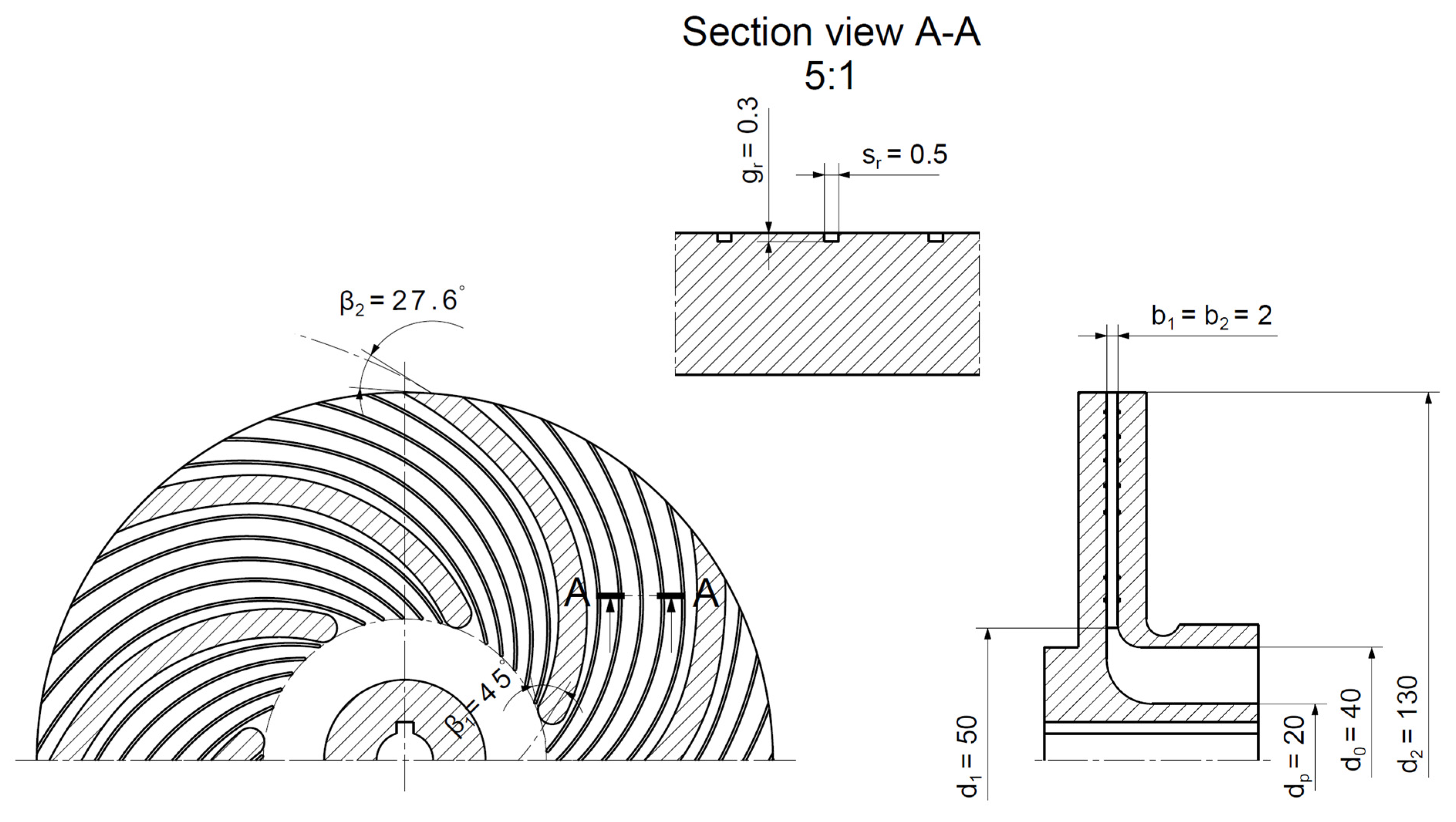
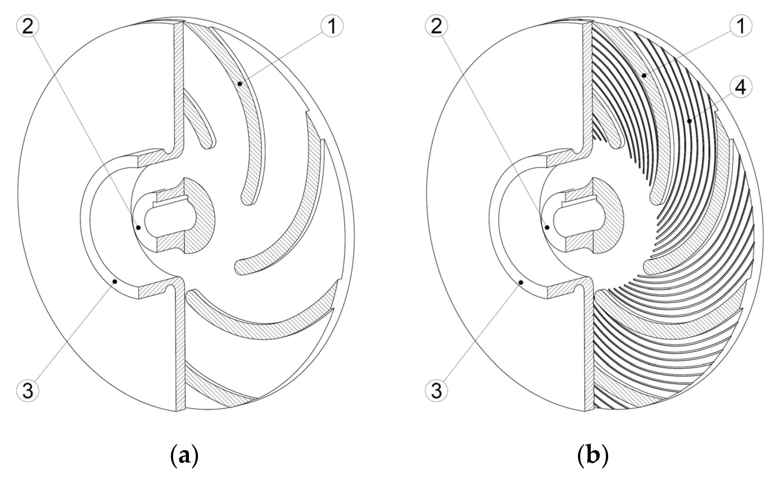
- The geometry of the main flow system of the impeller is unchanged (in both cases, there are the same: d1, d2, β1, β2, b1, b2).
- The cross-section of a groove is rectangular, with width sr and depth gr.
- The groove’s depth is constant along its entire length.
- The camber line of a groove corresponds to the camber line of a blade.
- The grooves are evenly distributed on the internal walls of the impeller.
- The grooves are made symmetrically inside the area between the impeller’s blades (there are the same number of grooves on the front and rear walls).
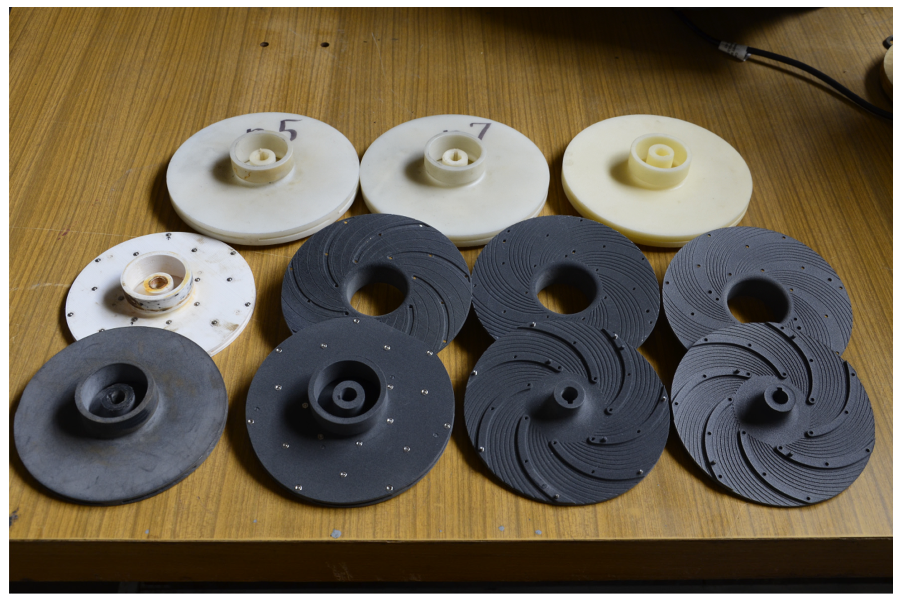
- The compared impellers are made of the same material using the same technology, which allows the same roughness to be obtained—comparable losses of the rotating discs.
2.2. Dimensional Analysis
2.3. Experiment Plan

| Parameter Name | Symbol | Minimal Value | Maximal Value | Value of the Change | Central Point |
|---|---|---|---|---|---|
| Thickness | gr, mm | 0.10 | 0.5 | 0.13 | 0.30 |
| Width | sr, mm | 0.25 | 0.75 | 0.17 | 0.50 |
| Number of grooves | zr, pcs. | 3 | 7 | 1.33 | 5 |
3. Research Methods
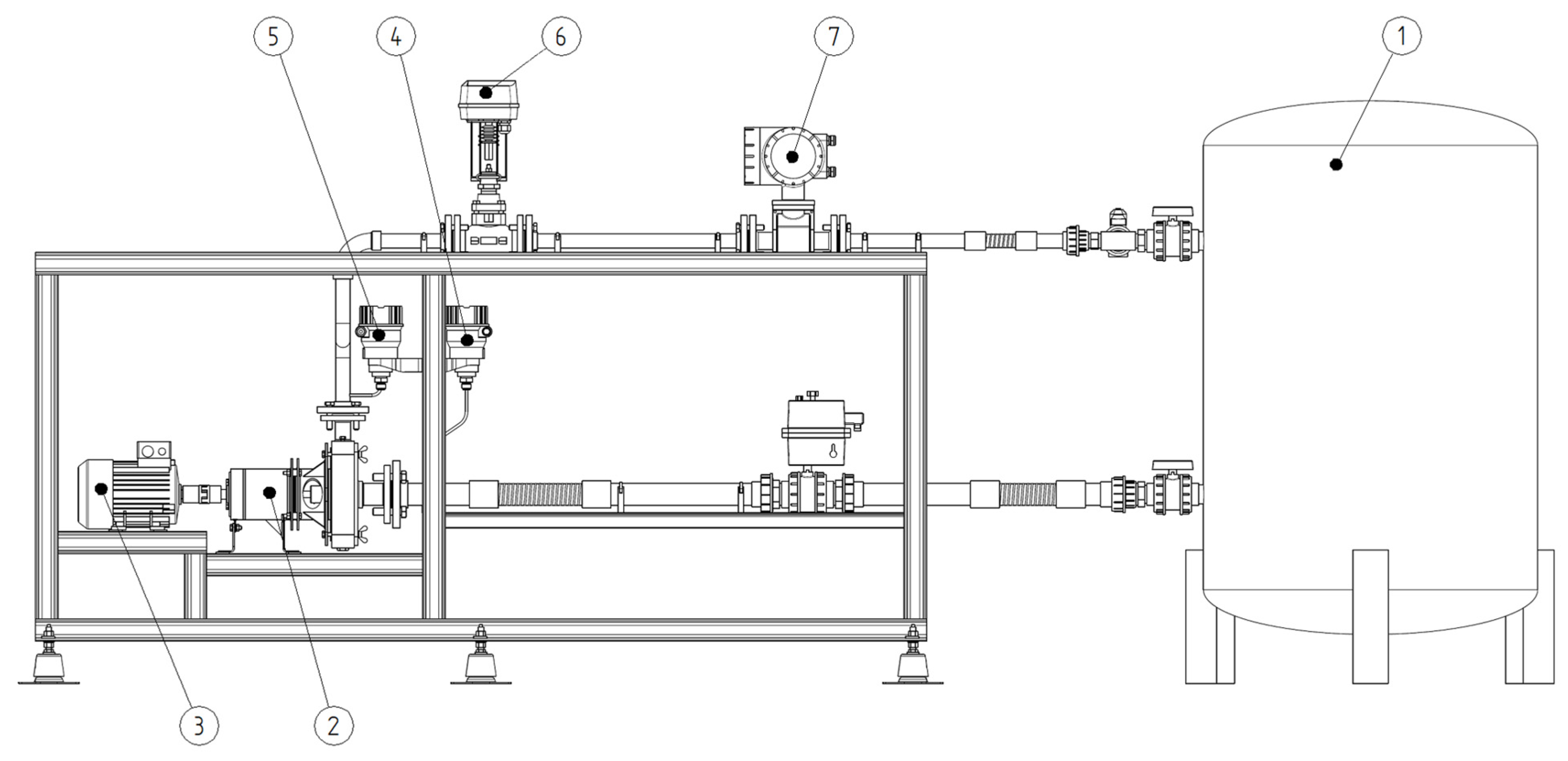
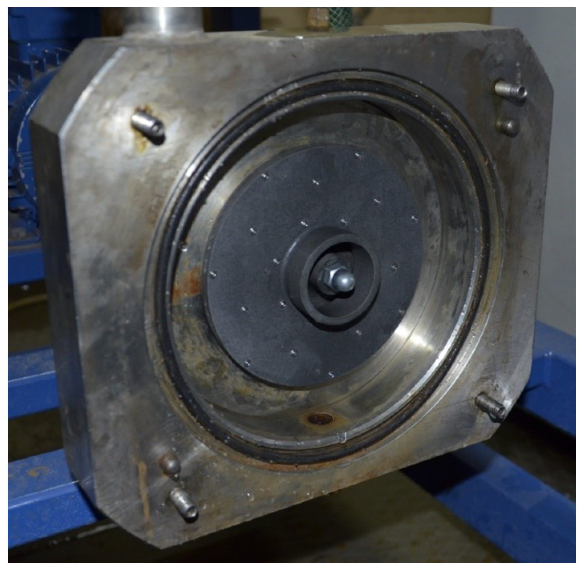
3.1. Test Stand and Measurement Procedures
3.2. Numerical Calculations
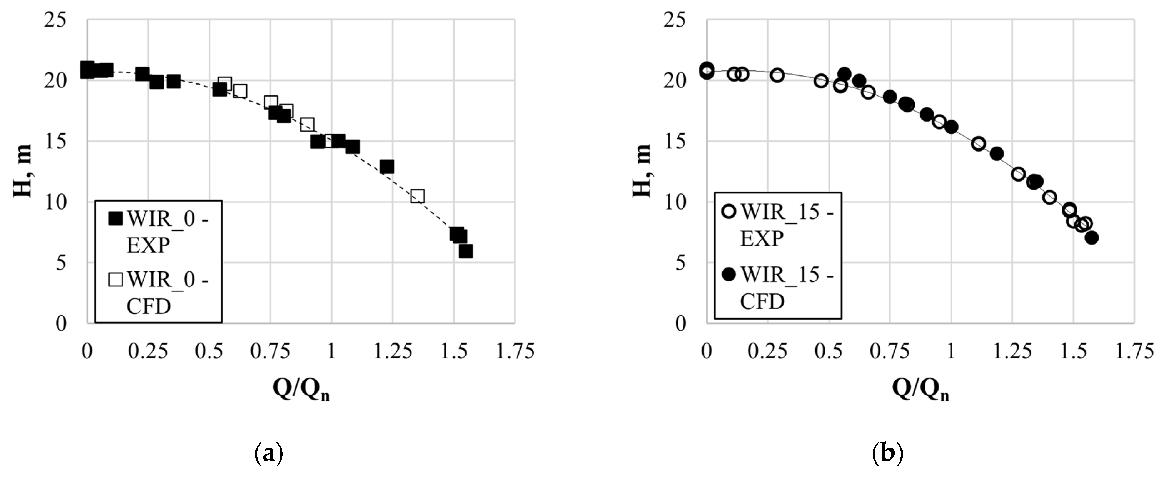
3.3. Verification of the Numerical Calculations
4. Results
4.1. Numerical Calculation Results for Qn
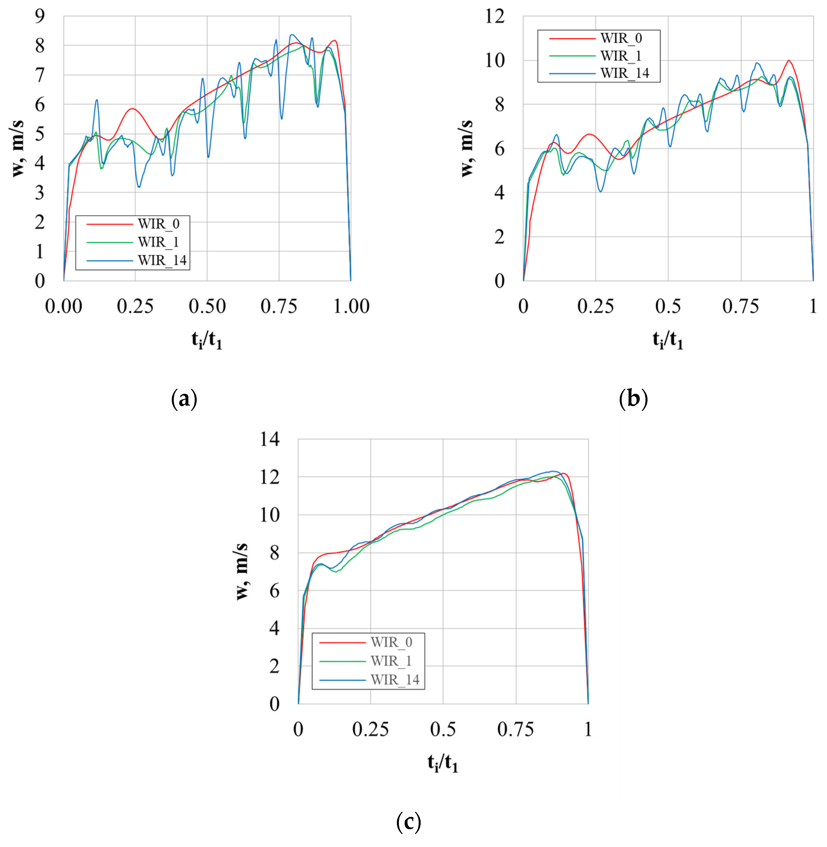
4.2. Speed Distributions in the Numerical Calculations for Qn
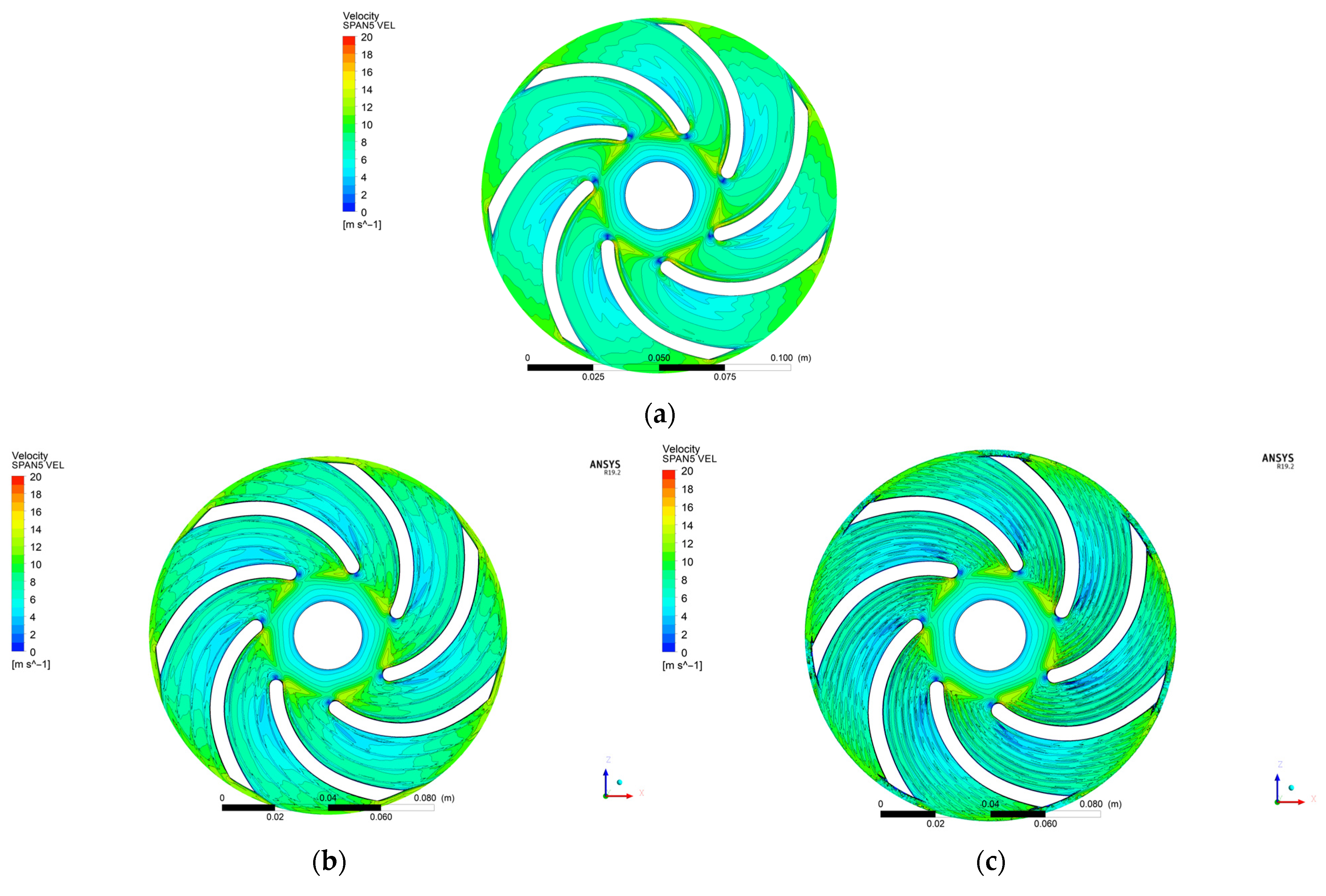
- The impact of a groove can be noticed in the distributions in the characteristic “break” of the speed profile—the maximum drop in speed is in the geometric center of the groove.
- The influence of the grooves on the flow is particularly visible near the wall near the active side of the blade (Figure 13a)—the speed profiles of the impellers with microgrooves are characterized by having low relative speed values.
- The graphs show the influence of the number of grooves on the speed distribution. In the case of the WIR_1 impeller, which has four grooves, four distinct depressions are visible on the speed profiles (Figure 13a), whereas in the case of the WIR_14 impeller, seven of them are visible (the impeller has seven grooves).
- The effect of groove depth can be seen by analyzing the depth of the speed profile’s “breaks”. It was observed that the higher the value of gr, the greater the variability of the speed profile (for WIR_1 gr = 0.17 mm and for WIR_14 gr = 0.3 mm).
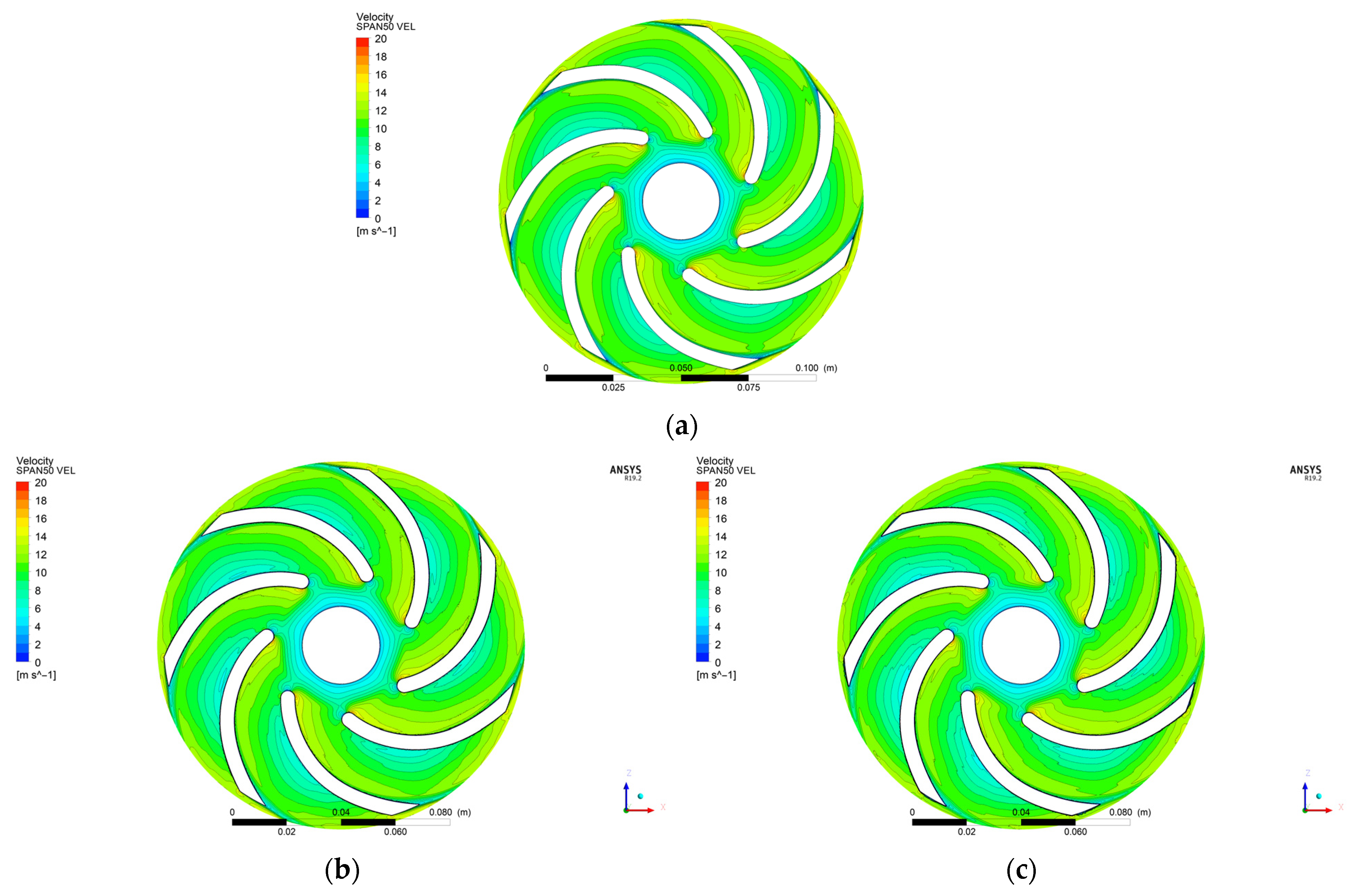
- The graphs show that the deeper the groove, the greater its impact on the speed field in the inter-blade channel, and this is especially visible when moving away from the wall. On the SPAN10 control plane, the peaks in the speed distribution, which were determined for WIR_14, are characterized by having a larger amplitude than those obtained for the impeller with a smaller depth of the grooves (Figure 13b).
- On the control plane located exactly in the middle of the impeller’s channel, it can be seen that the influence of the grooves is already very weak (Figure 13c). The speed profiles are very similar to each other, and only a slight distortion of the speed profiles is visible. However, the average speed values obtained for the impellers with microgrooves are lower than those obtained for the smooth impeller.
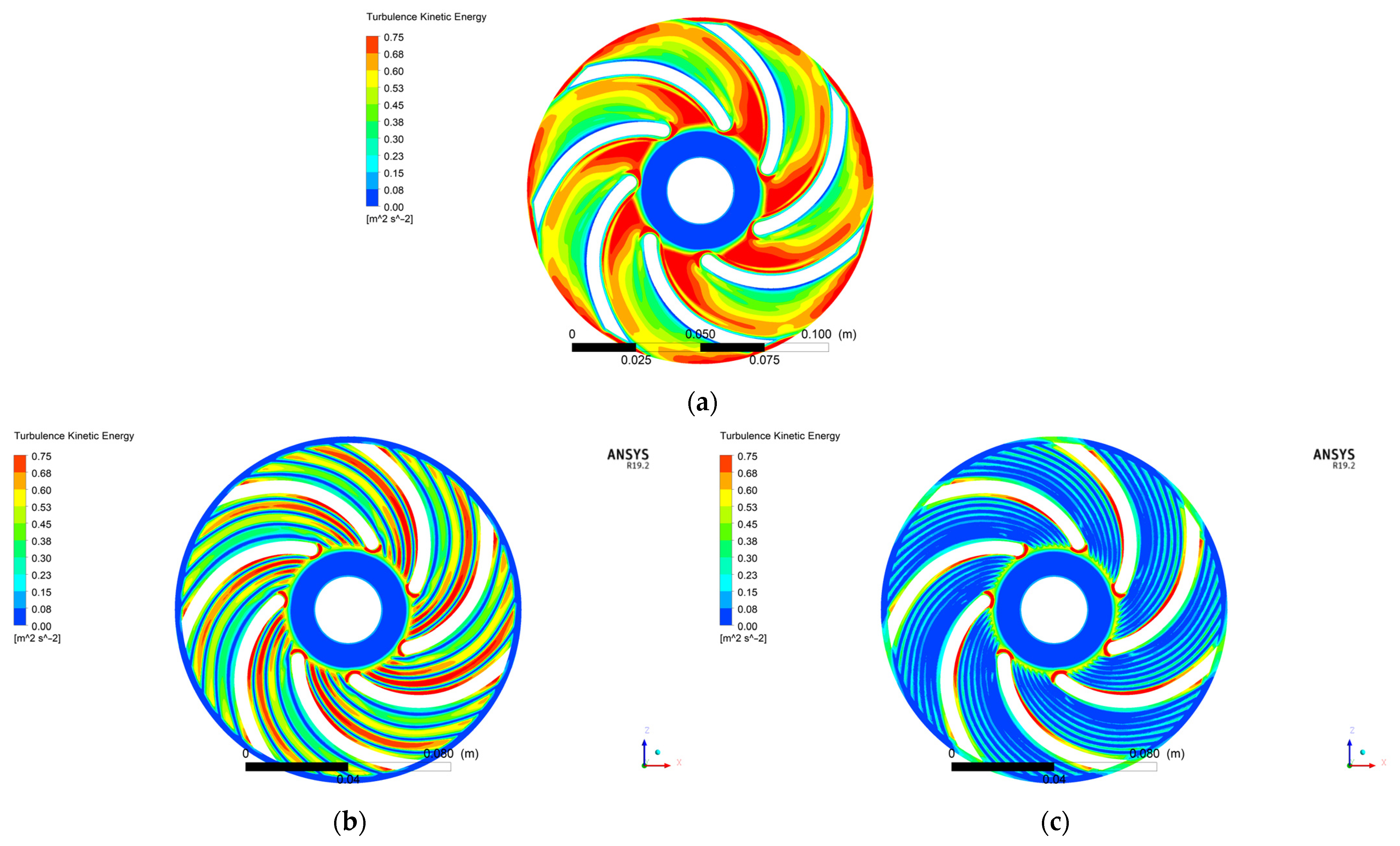
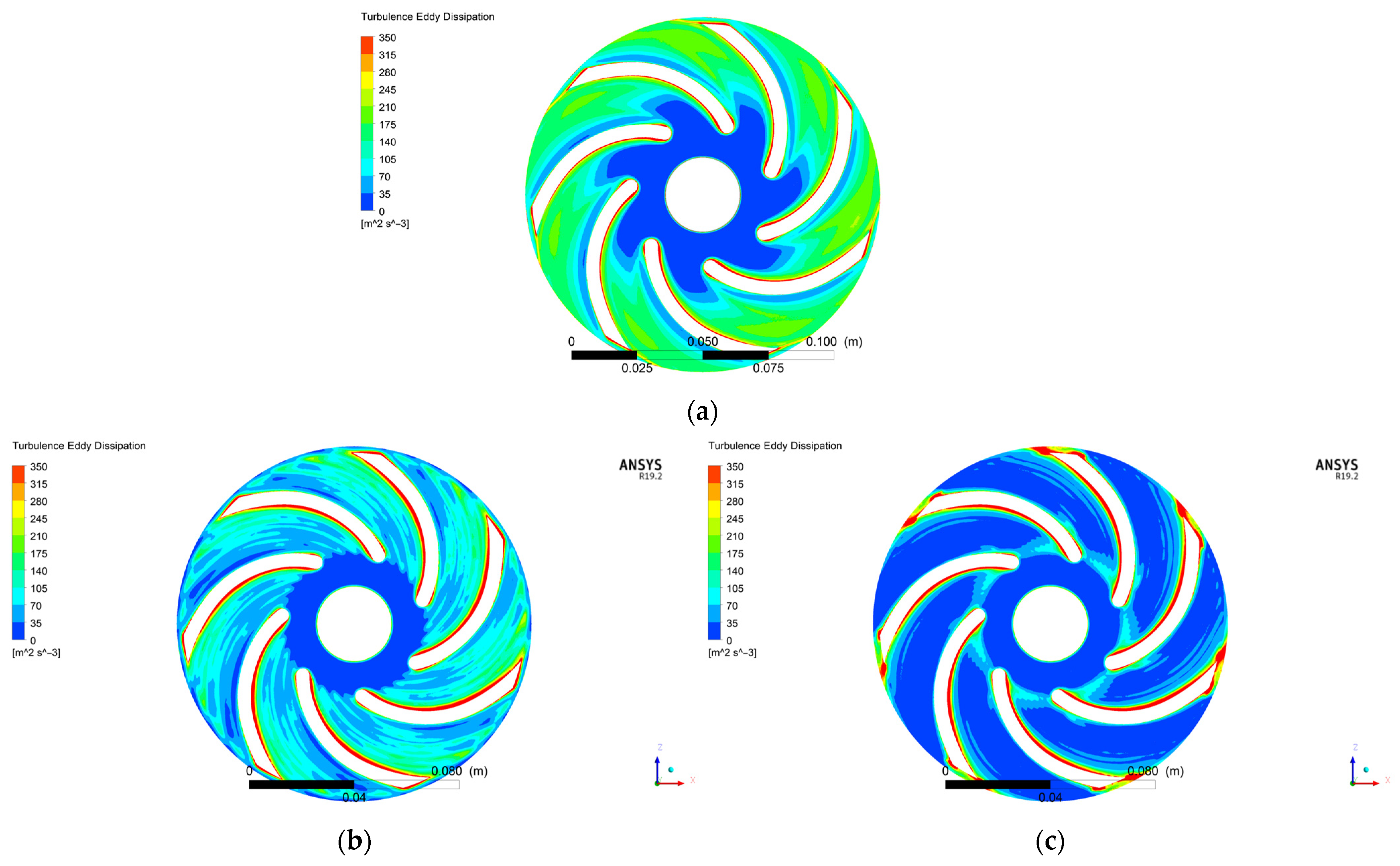
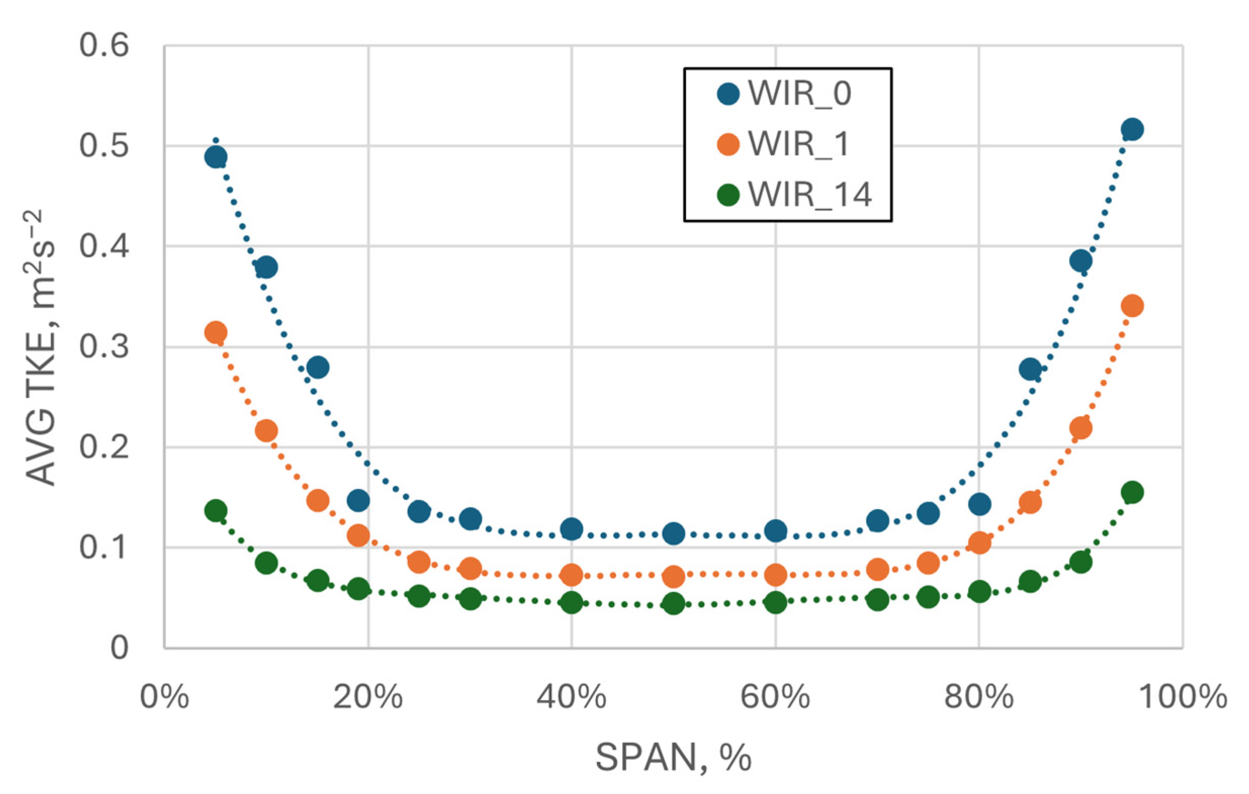
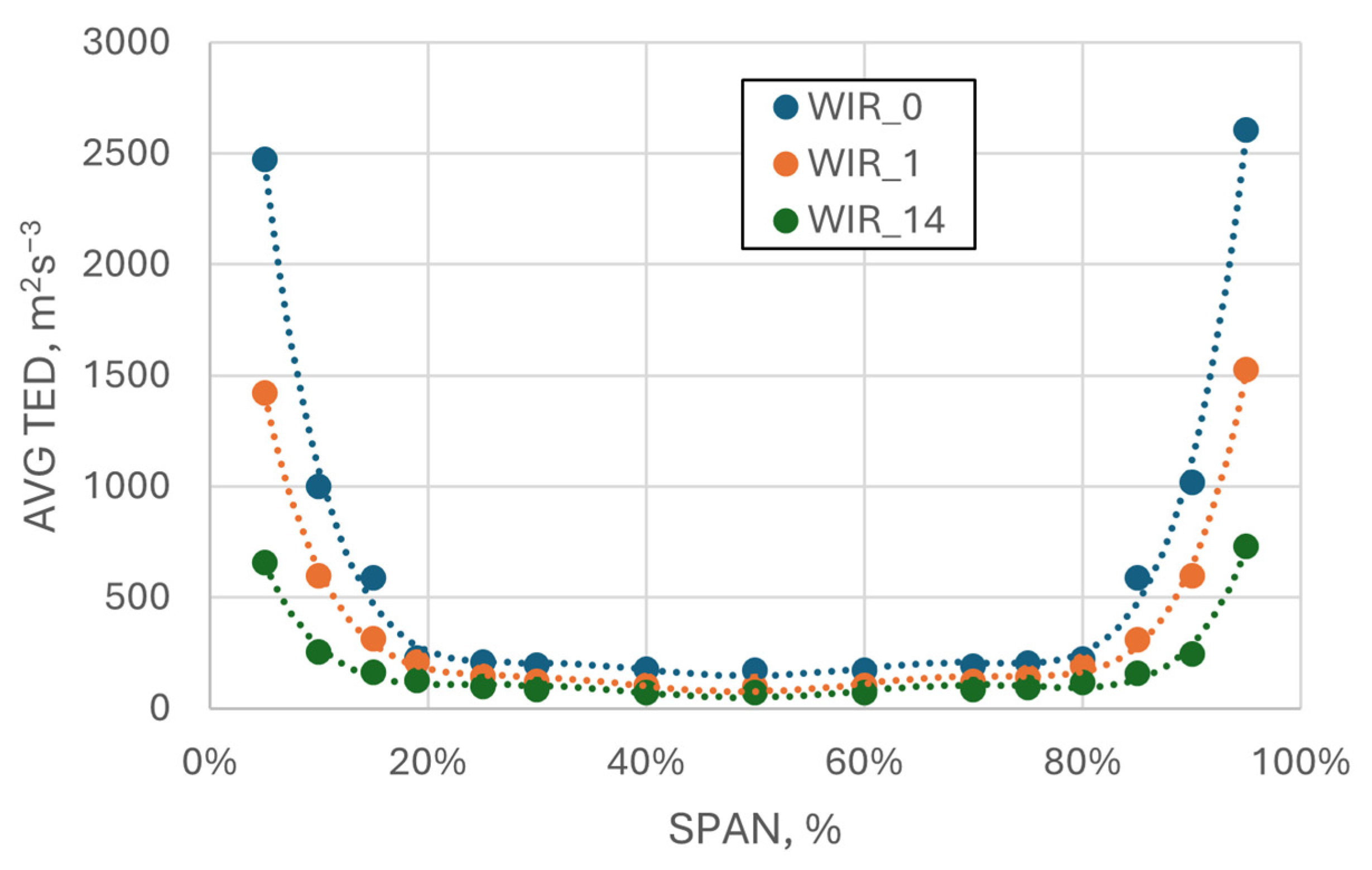
4.3. Analysis of the TKE and TED Distributions
5. Guidelines for Designing Impellers with Microgrooves
6. Summary and Conclusions
- Numerical fluid dynamics can be treated as a reliable research tool for modeling and analyzing flow phenomena that occur in pumps with microgrooves. The errors in estimating the lifting height near the optimal point do not exceed 3%.
- The use of microgeometry has a beneficial effect on a reduction in internal flow losses by reducing the area of impact of the boundary layer. The use of grooves allowed the area of impact of the boundary layer to be reduced by approximately 20%.
- It can be concluded that the influence of the groove’s depth gr has the most significant impact on flow parameters. This is strongly related to the thickness of the boundary layer. In order for the use of microgeometry to make sense, the area of the negative influence of the boundary layer must constitute a significant part of the flow channel (losses in the boundary layer must constitute a significant part of the losses occurring in the inter-blade channel). For this reason, the possibilities of using grooves are limited to narrow impellers (nq < 15 and Q < 10 m3/h).
- It was noticed that the influence of the groove on the speed distribution depends on the groove’s depth, and it decreases with decreasing depth.
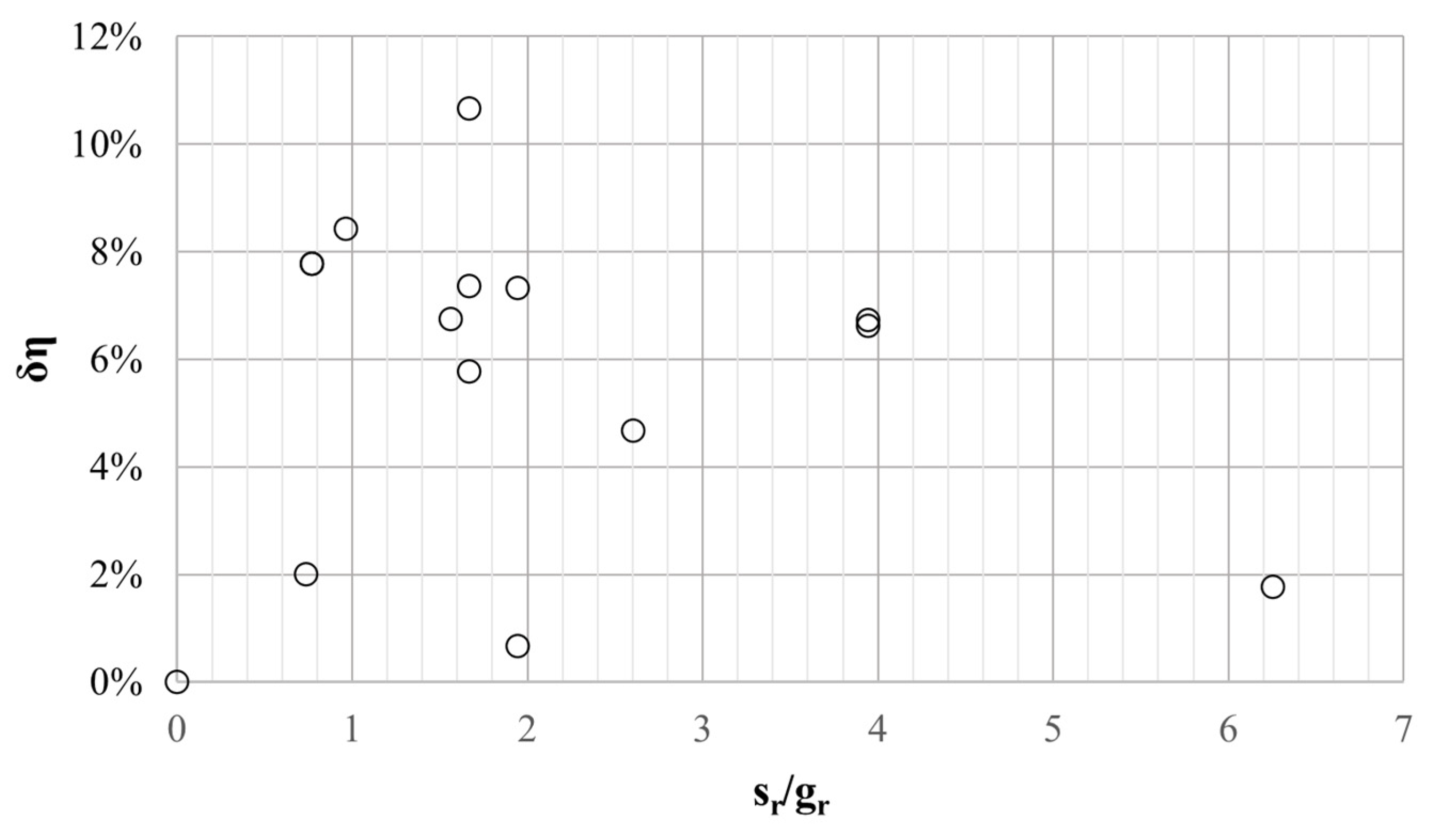
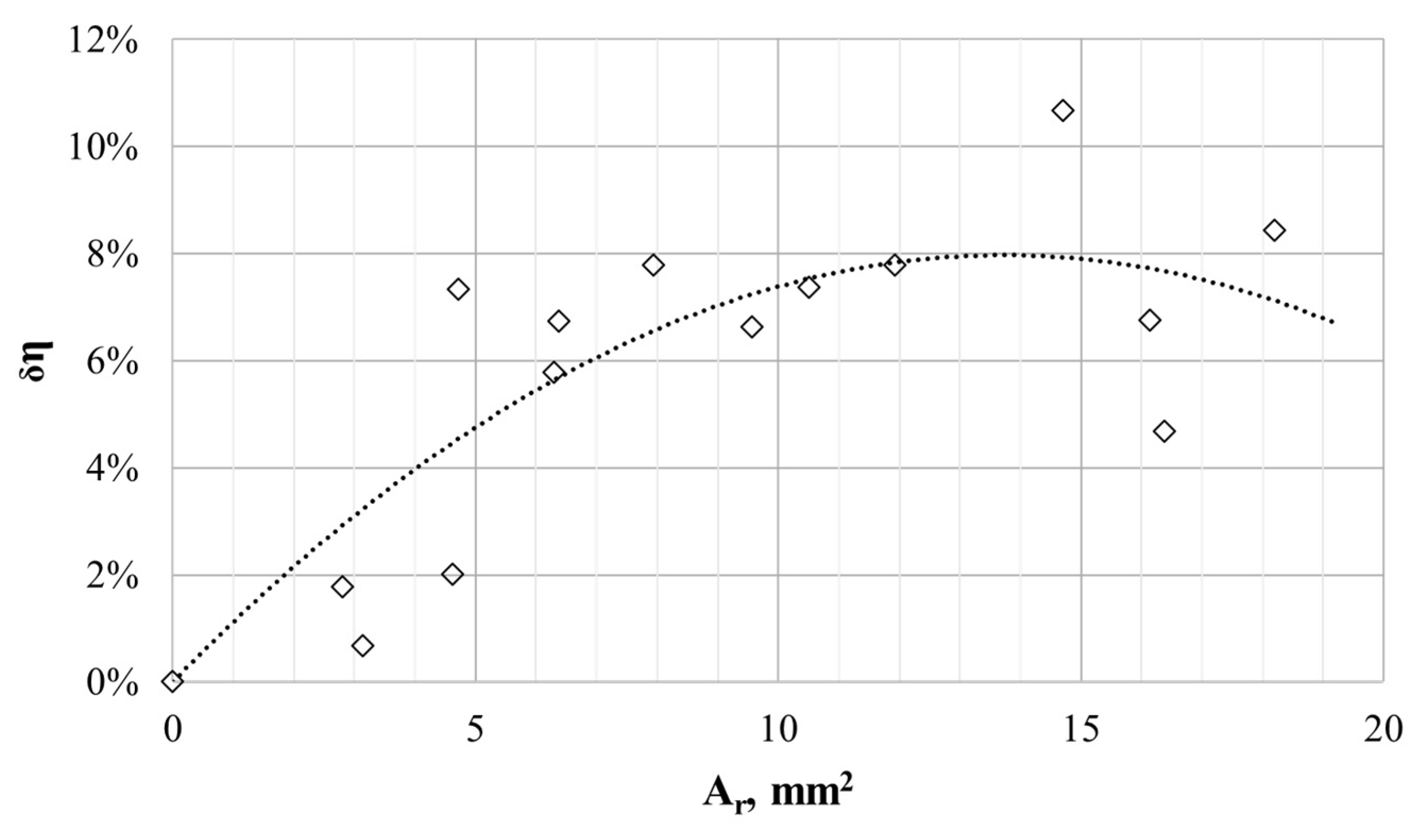
- The optimal ratio of the impeller’s outlet cross-sectional area to the grooves’ cross-sectional area was determined.
Author Contributions
Funding
Data Availability Statement
Acknowledgments
Conflicts of Interest
Nomenclature
| Symbol | Name | Unit |
| a | star arm | - |
| Ar | cross-sectional area of all the grooves | mm2 |
| A2 | impeller outlet cross-section area | mm2 |
| b1 | impeller width at the inlet | mm |
| b2 | impeller width impeller width at the outlet | mm |
| b3 | annular casing width | mm |
| d1 | impeller inlet diameter | mm |
| d2 | impeller outlet diameter | mm |
| d3 | annular casing diameter | mm |
| g | gravity acceleration | m/s2 |
| gr | groove depth | mm |
| H | pump lifting height | m |
| M | total torque on the moving walls of the impeller | Nm |
| n | rotational speed | rpm |
| nq | kinematic specific speed factor | - |
| N | number of experiments in the experiment plan | - |
| S | number of independent variables | - |
| sr | groove width | mm |
| Pw | power input | W |
| Q | capacity | m3/h |
| R2 | determination coefficient | - |
| T | temperature | °C |
| t | time | s |
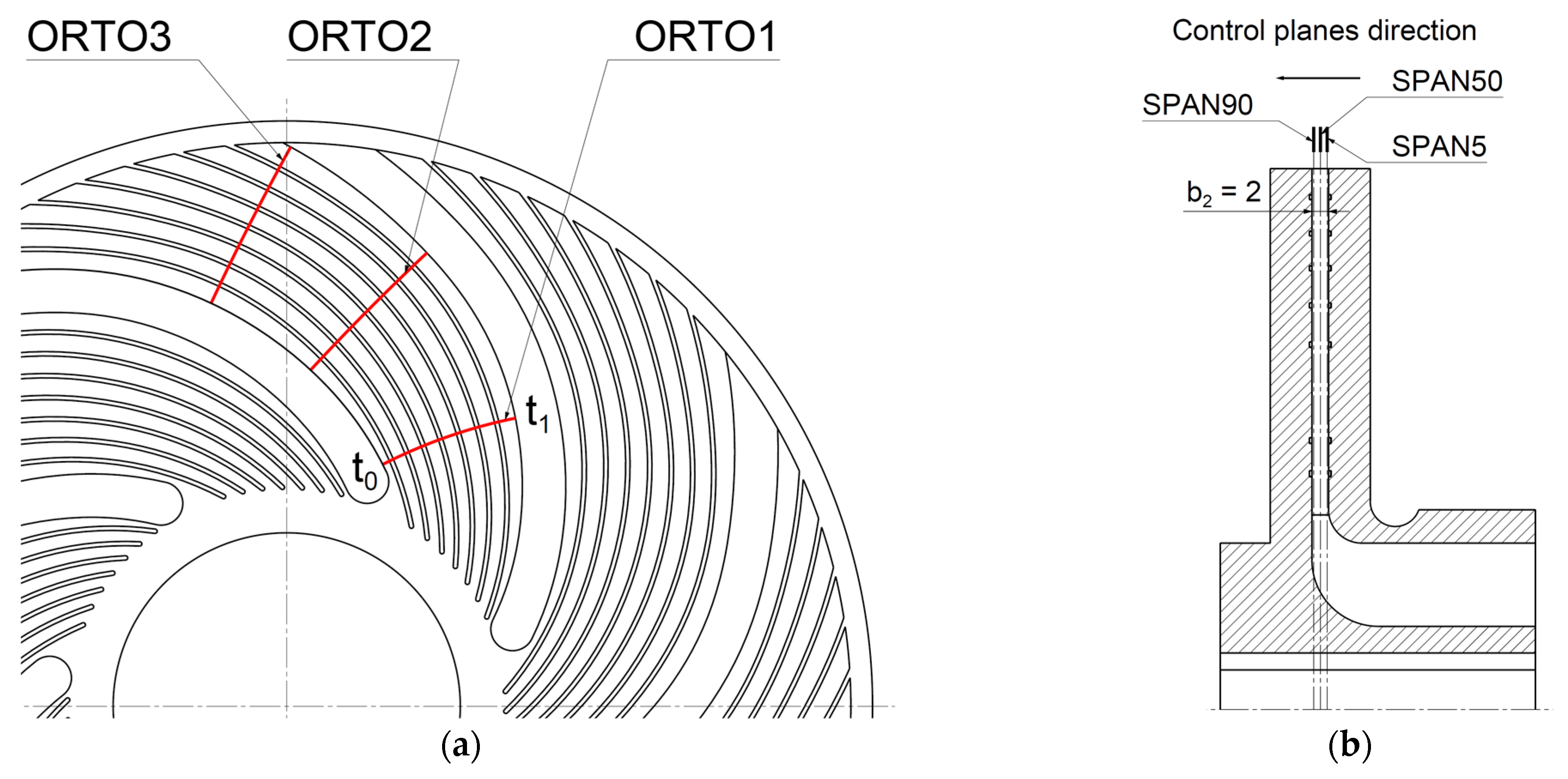
| t0 | active side of the blade | - |
| t1 | passive side of the blade | - |
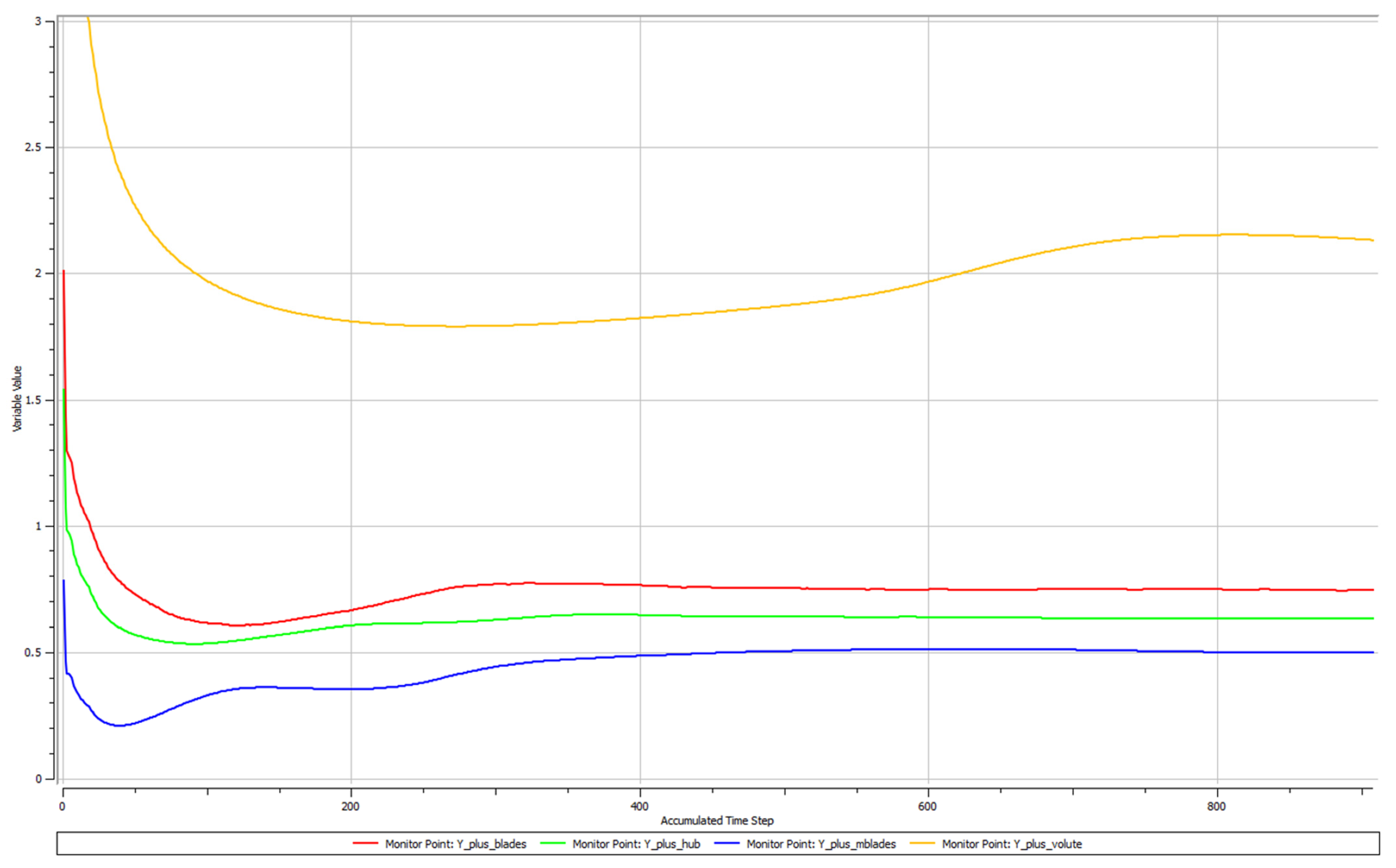
| y+ | Reynolds number in cell | - |
| Y | unit energy | J |
| z | number of impeller flow channels | - |
| zr | number of grooves | - |
| zrc | total number of grooves | - |
| Greek Symbols | ||
| β | inflow angle, offset angle | ° |
| δ | relative error, relative increase | - |
| Δ | variability, difference | - |
| ζr | area ratio | - |
| η | efficiency | - |
| μ | dynamic viscosity coefficient | Pa·s |
| ν | kinematic viscosity coefficient | m2/s |
| π | number, dimensionless variable | - |
| ρ | fluid density | kg/m3 |
| ω | angular velocity | rad/s |
| Subscripts | ||
| CFD | Computational Fluid Dynamics, applies to results obtained using CFD | - |
| EXP | experimental | - |
| h | hydraulic | - |
| H2O | applies to water | - |
| i | next value | - |
| n | nominal | - |
| opt | optimal | - |
References
- Skrzypacz, J. Investigating the impact of multi-piped impellers design on the efficiency of rotodynamic pumps operating at ultra-low specific speed. Chem. Eng. Process. 2004, 86, 145–152. [Google Scholar] [CrossRef]
- Skrzypacz, J. Numerical modelling of flow phenomena in a pump with a multi-piped impeller. Chem. Eng. Process. 2014, 75, 58–66. [Google Scholar] [CrossRef]
- Skrzypacz, J. Impeller of an impeller pump (Wirnik pompy wirowej). Patent PL 210647 B1, 25 August 2011. [Google Scholar]
- Skrzypacz, J.; Bieganowski, M. The influence of micro grooves on the parameters of the centrifugal pump impeller. Int. J. Mech. Sci. 2018, 144, 827–835. [Google Scholar] [CrossRef]
- Barenblatt, G.I. Dimensional Analysis and Intermediate Asymptotics; Cambridge University Press: Cambridge, UK, 1996. [Google Scholar]
- Kasprzak, W.; Lysik, B. Dimensional Analysis in Experiment Design; Zakład Narodowy im. Ossolińskich—Wydawnictwo Polskiej Akademii Nauk: Wroclaw, Poland, 1978. [Google Scholar]
- Kasprzak, W.; Lysik, B. Dimensional Analysis: Algorithmic Procedures for Experiment Management; Wydawnictwa Naukowo–Techniczne: Warsaw, Poland, 1988. [Google Scholar]
- Müller, L. Application of Dimensional Analysis in Model Research; Państwowe Wydawnictwo Naukowe: Warsaw, Poland, 1983. [Google Scholar]
- Roslanowski, J. Valuation of rotodynamic pumps operation, by means of, dimensional analysis. J. Pol. CIMAC 2014, 9, 73–80. [Google Scholar]
- Siedow, L.I. Dimensional Analysis and Similarity Theory in Mechanics; Wydawnictwa Naukowo–Technicze: Warsaw, Poland, 1968. [Google Scholar]
- Szirtes, T. Applied Dimensional Analysis and Modeling; McGraw-Hill: New York, NY, USA, 1997. [Google Scholar]
- Gülich, J.F. Centriflugal Pumps, 2nd ed.; Springer: Berlin/Heidelberg, Germany, 2010. [Google Scholar]
- Łazarkiewicz, S.; Troskolański, A.T. Modern Trends in the Construction of Centrifugal Pumps; Wydawnictwa Naukowo–Techniczne: Warsaw, Poland, 1966. [Google Scholar]
- Troskolański, A.T.; Łazarkiewicz, S. Centriflugal Pumps; Wydawnictwa Naukowo–Techniczne: Warsaw, Poland, 1973. [Google Scholar]
- Kacprzyński, B. Planning Experiments: Mathematical Foundations; Wydawnictwa Naukowo–Techniczne: Warsaw, Poland, 1974. [Google Scholar]
- Mańczak, K. Experiment Planning Technique; Wydawnictwa Naukowo–Techniczne: Warsaw, Poland, 1976. [Google Scholar]
- Korzyński, M. Experiment Methodology: Planning, Implementation and Statistical Analysis of Experimental Results, 2nd ed.; WNT: Warsaw, Poland, 2017. [Google Scholar]
- Polański, Z. Planning Experiments in Technology; Państwowe Wydawnictwo Naukowe: Warsaw, Poland, 1984. [Google Scholar]
- Si, Q.; Yuan, S.; Yuan, J.; Wang, C.; Lu, W. Multiobjective Optimization of Low-Specific-Speed Multistage Pumps by Using Matrix Analysis and CFD Method. J. Appl. Math. 2013, 2013, 136195. [Google Scholar] [CrossRef]
- Li, Z.; Ding, H.; Shen, X.; Jiang, Y. Performance Optimization of High Specific Speed Centrifugal Pump Based on Orthogonal Experiment Design Method. Processes 2019, 7, 728. [Google Scholar] [CrossRef]
- EN ISO 9906:2012; Rotodynamic Pumps—Hydraulic Performance, Acceptance Tests—Grades 1, 2 and 3. International Organization for Standardization: Geneva, Switzerland, 2012.
- ANSYS, Inc. ANSYS CFX–Solver Modeling Guide. Release 18.0; ANSYS, Inc.: Canonsburg, PA, USA, 2017. [Google Scholar]
- Menter, F.; Kuntz, M.; Langtry, R. Ten years of industrial experience with the SST turbulence model. Turbul. Heat Mass Transf. 2003, 4, 625–632. [Google Scholar]
- Menter, F.R.; Ferreira, J.C.; Esch, T.; Konno, B. The SST Turbulence Model with Improved Wall Treatment for Heat Transfer Predictions in Gas Turbines. In Proceedings of the International Gas Turbine Congress 2003, Tokyo, Japan, 2–7 November 2003. [Google Scholar]
- Salim, M.S.; Cheah, C.S. Wall y+ Strategy for Dealing with Wall-bounded Turbulent Flows. In Proceedings of the International Multi Conference of Engineers and Computer Scientists, Hong Kong, 18–20 March 2009; Volume 2. [Google Scholar]
- ANSYS, Inc. ANSYS CFX Theory Guide. Release 16.2; ANSYS, Inc.: Canonsburg, PA, USA, 2016. [Google Scholar]
- Wileox, D.C. Turbulence Modelling for CFD, 3rd ed.; DCW Industries: San Diego, CA, USA, 2006. [Google Scholar]

| Set Number | gr, mm | sr, mm | zr, pc. (Rounded up) | zrc, pc. |
|---|---|---|---|---|
| WIR_1 | 0.17 | 0.33 | 4 | 56 |
| WIR_2 | 0.43 | 0.33 | 4 | 56 |
| WIR_3 | 0.17 | 0.67 | 4 | 56 |
| WIR_4 | 0.43 | 0.67 | 4 | 56 |
| WIR_5 | 0.17 | 0.33 | 6 | 84 |
| WIR_6 | 0.43 | 0.33 | 6 | 84 |
| WIR_7 | 0.17 | 0.67 | 6 | 84 |
| WIR_8 | 0.43 | 0.67 | 6 | 84 |
| WIR_9 | 0.08 | 0.50 | 5 | 70 |
| WIR_10 | 0.52 | 0.50 | 5 | 70 |
| WIR_11 | 0.30 | 0.22 | 5 | 70 |
| WIR_12 | 0.30 | 0.78 | 5 | 70 |
| WIR_13 | 0.30 | 0.50 | 3 | 42 |
| WIR_14 | 0.30 | 0.50 | 7 | 98 |
| WIR_15 | 0.30 | 0.50 | 5 | 70 |
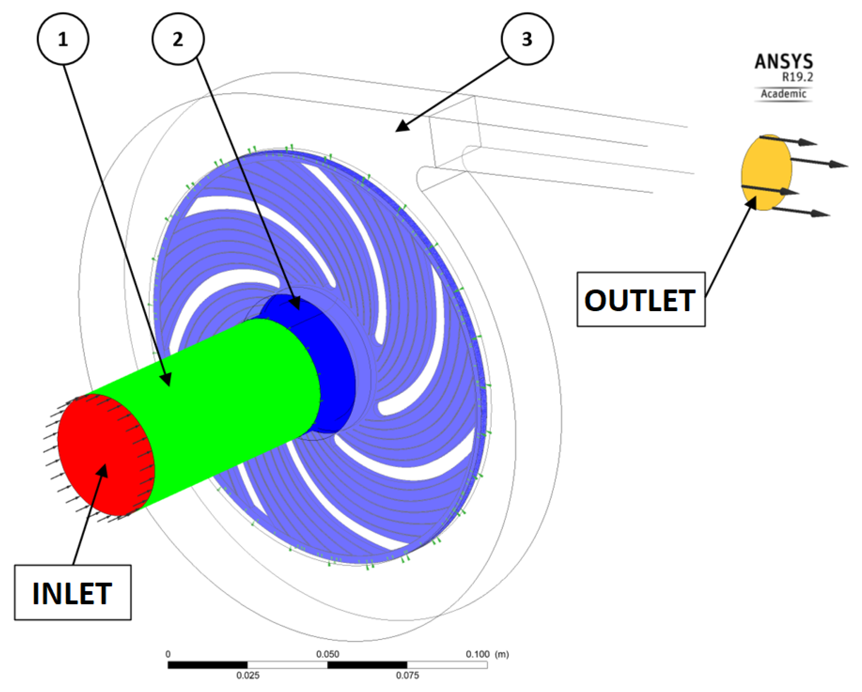
| No. | Initial Condition | Setting |
|---|---|---|
| 1 | Inlet | Gradientless inflow, constant static pressure |
| 2 | Outlet | Mass flow—in the case of constant density, it is equivalent to the velocity condition (rectangular velocity profile, Dirichlet condition) |
| 3 | Impeller’s domain | Rotation speed n = 2950 rotations/min |
| 4 | Liquid | Water with density = 998.2 kg/m3 and viscosity = 0.001003 Pa·s |
| 5 | Temperature | Isothermal calculations, T = 20 °C |
| 6 | Fixed walls | No-slip condition, zero speed on the wall |
| 7 | Movable walls | No-slip condition, zero speed on the wall, n = 2950 rotations/min |
| 8 | Convergence | Minimum level of convergence of the stationary calculations equal to 10−4 |
| 9 | Advection Scheme | High Resolution |
| 10 | Turbulence Numerics | High Resolution |
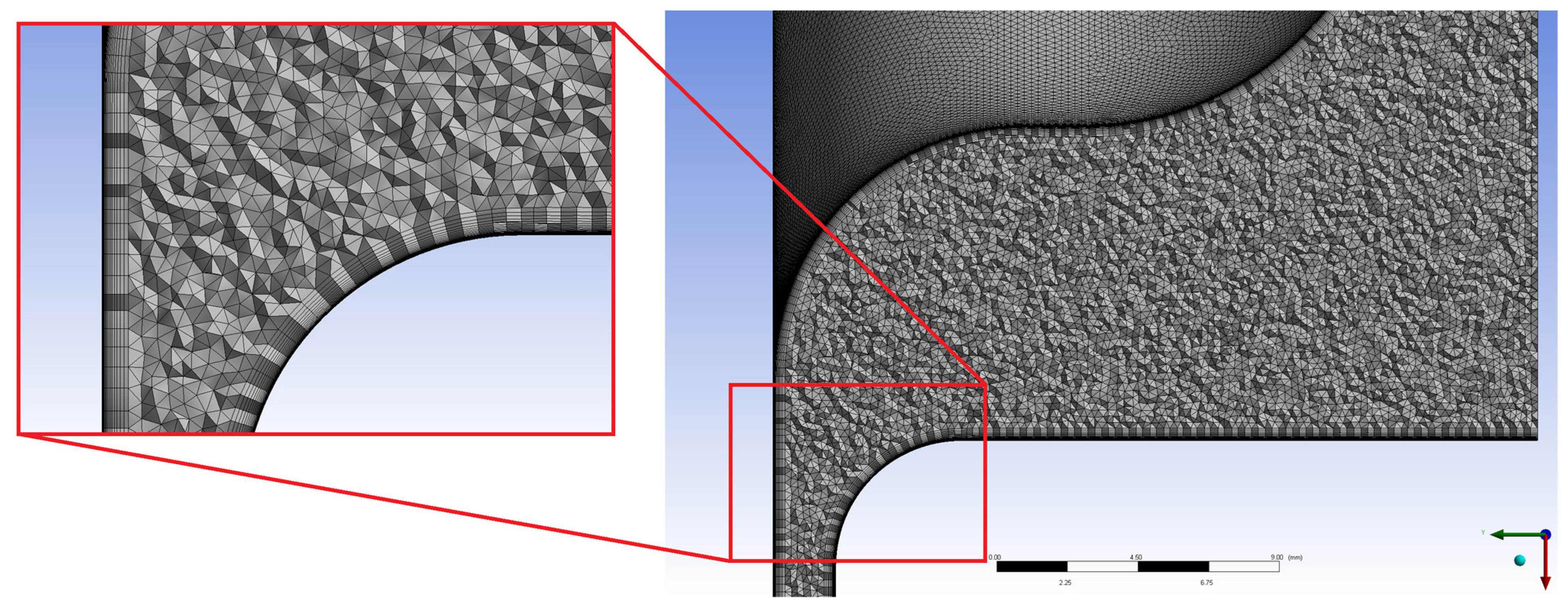
| Impeller | Number of Elements | Average Quality | Average Skewness | Aspect Ratio (Average) |
|---|---|---|---|---|
| WIR_0 (without grooves) | 46,472,396 | 0.79715 | 0.20648 | 2.0746 |
| WIR_1 (the smallest number of grooves) | 72,213,142 | 0.8213 | 0.20785 | 2.0312 |
| WIR_14 (the largest number of grooves) | 106,056,646 | 0.81965 | 0.21698 | 1.9301 |
| Set Number | H, m | ΔH, m | δH, % | η, % | Δη, % | δη, % |
|---|---|---|---|---|---|---|
| WIR_0 | 15.03 | - | - | 35.16% | - | - |
| WIR_1 | 15.65 | 0.622 | 4.14% | 35.40% | 0.24% | 0.68% |
| WIR_2 | 16.21 | 1.182 | 7.86% | 37.90% | 2.74% | 7.79% |
| WIR_3 | 15.98 | 0.953 | 6.34% | 37.53% | 2.37% | 6.75% |
| WIR_4 | 16.57 | 1.546 | 10.29% | 37.54% | 2.38% | 6.76% |
| WIR_5 | 15.71 | 0.683 | 4.54% | 37.74% | 2.58% | 7.33% |
| WIR_6 | 16.21 | 1.178 | 7.84% | 37.90% | 2.74% | 7.78% |
| WIR_7 | 15.97 | 0.941 | 6.26% | 37.49% | 2.33% | 6.63% |
| WIR_8 | 15.42 | 0.39 | 2.59% | 35.45% | 0.29% | 0.82% |
| WIR_9 | 15.51 | 0.487 | 3.24% | 35.77% | 0.63% | 1.78% |
| WIR_10 | 16.51 | 1.485 | 9.88% | 38.13% | 2.97% | 8.44% |
| WIR_11 | 15.69 | 0.667 | 4.44% | 35.87% | 0.71% | 2.01% |
| WIR_12 | 15.91 | 0.88 | 5.85% | 36.80% | 1.64% | 4.68% |
| WIR_13 | 16.02 | 0.99 | 6.59% | 37.19% | 2.04% | 5.79% |
| WIR_14 | 16.16 | 1.127 | 7.50% | 38.91% | 3.75% | 10.67% |
| WIR_15 | 16.15 | 1.116 | 7.43% | 37.75% | 2.59% | 7.38% |
| Control Plane | Impeller Designation | Averaged Speed [m/s] |
|---|---|---|
| SPAN5 | WIR_0 | 7.542 |
| WIR_1 | 7.309 | |
| WIR_14 | 7.233 | |
| SPAN50 | WIR_0 | 10.152 |
| WIR_1 | 9.962 | |
| WIR_14 | 9.959 |
Disclaimer/Publisher’s Note: The statements, opinions and data contained in all publications are solely those of the individual author(s) and contributor(s) and not of MDPI and/or the editor(s). MDPI and/or the editor(s) disclaim responsibility for any injury to people or property resulting from any ideas, methods, instructions or products referred to in the content. |
© 2024 by the authors. Licensee MDPI, Basel, Switzerland. This article is an open access article distributed under the terms and conditions of the Creative Commons Attribution (CC BY) license (https://creativecommons.org/licenses/by/4.0/).
Share and Cite
Bieganowski, M.; Skrzypacz, J.; Chomiuk, B. The Influence of the Geometry of Grooves on the Operating Parameters of the Impeller in a Centrifugal Pump with Microgrooves. Energies 2024, 17, 2807. https://doi.org/10.3390/en17122807
Bieganowski M, Skrzypacz J, Chomiuk B. The Influence of the Geometry of Grooves on the Operating Parameters of the Impeller in a Centrifugal Pump with Microgrooves. Energies. 2024; 17(12):2807. https://doi.org/10.3390/en17122807
Chicago/Turabian StyleBieganowski, Marcin, Janusz Skrzypacz, and Bartłomiej Chomiuk. 2024. "The Influence of the Geometry of Grooves on the Operating Parameters of the Impeller in a Centrifugal Pump with Microgrooves" Energies 17, no. 12: 2807. https://doi.org/10.3390/en17122807
APA StyleBieganowski, M., Skrzypacz, J., & Chomiuk, B. (2024). The Influence of the Geometry of Grooves on the Operating Parameters of the Impeller in a Centrifugal Pump with Microgrooves. Energies, 17(12), 2807. https://doi.org/10.3390/en17122807