

A Novel Method to Calculate Water Influx Parameters and Geologic Reserves for Fractured-Vuggy Reservoirs with Bottom/Edge Water

Abstract
:1. Introduction
2. Establishment of Water Influx Characteristic Model
2.1. Calculation of Pore Space Reduction Volume and Water Expansion Volume in Waterbody
2.2. Derivation of the Relationship between the Net Water Influx and Cumulative Oil Production
3. Calculation of Water Influx and OOIP
3.1. Establishment of Material Balance Equation
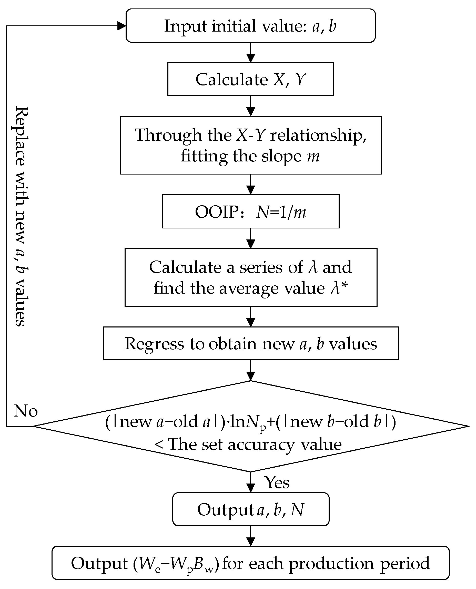
3.2. Equation Solving
4. Method Validation
5. Application of the Developed Method to a Field Case
6. Conclusions
- (1)
- The calculation method is sensitive to the values of reservoir pressure and crude oil formation volume factor. Significant errors in reservoir static pressure tests and calculation errors in the oil formation volume factor may lead to the non-convergence of calculation results;
- (2)
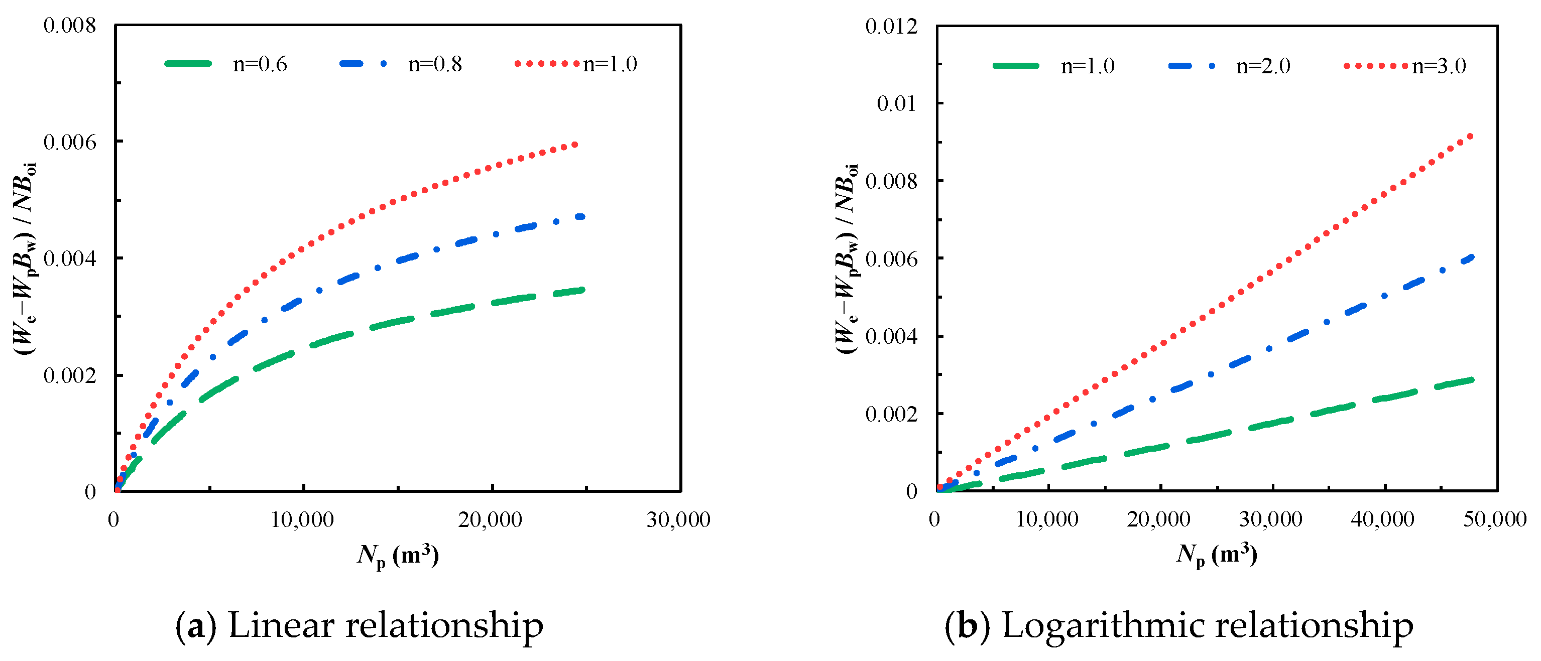
- Water influx for fractured-vuggy carbonate reservoirs with bottom/edge water can be characterized into two types, logarithmic water influx and linear water influx. In the early stages of water influx, the water influx rate of logarithmic water influx often exceeds that of linear water influx;
- (3)
- For logarithmic water influx wells, the volume of the connected waterbody is relatively small, and the energy of the waterbody is weak. Water influx phenomena typically occur only within a short period after water movement. In contrast, for linear water influx wells, the volume of the connected waterbody is larger, and the energy of the waterbody can sustain a stable water influx rate.
- (4)
- The determination method of the aquifer to hydrocarbon ratio for fracture-vuggy carbonate reservoirs with bottom water, as well as related research findings on OOIP and the prediction of water invasion patterns, can provide theoretical support for the evaluation of waterbody energy, dynamic analysis of water invasion, and water control and management for such reservoirs.
Author Contributions
Funding
Data Availability Statement
Conflicts of Interest
References
- Tan, Y.; Li, Q.; Xu, L.; Ghaffar, A.; Zhou, X.; Li, P. A critical review of carbon dioxide enhanced oil recovery in carbonate reservoirs. Fuel 2022, 328, 125256. [Google Scholar] [CrossRef]
- Yao, Y.; Wei, M.; Kang, W. A review of wettability alteration using surfactants in carbonate reservoirs. Adv. Colloid Interface Sci. 2021, 294, 102477. [Google Scholar] [CrossRef]
- Xu, Z.X.; Li, S.Y.; Li, B.F.; Chen, D.Q.; Liu, Z.Y.; Li, Z.M. A review of development methods and EOR technologies for carbonate reservoirs. Pet. Sci. 2020, 17, 990–1013. [Google Scholar] [CrossRef]
- Wang, J.; Song, H.; Wang, Y. Investigation on the micro-flow mechanism of enhanced oil recovery by low-salinity water flooding in carbonate reservoir. Fuel 2020, 266, 117156. [Google Scholar] [CrossRef]
- Liu, B.; Jin, Y.; Chen, M. Influence of vugs in fractured-vuggy carbonate reservoirs on hydraulic fracture propagation based on laboratory experiments. J. Struct. Geol. 2019, 124, 143–150. [Google Scholar] [CrossRef]
- Wen, Y.C.; Hou, J.R.; Xiao, X.L.; Li, C.M.; Qu, M.; Zhao, Y.J.; Wu, W.P. Utilization mechanism of foam flooding and dis-tribution situation of residual oil in fractured-vuggy carbonate reservoirs. Pet. Sci. 2023, 20, 1620–1639. [Google Scholar] [CrossRef]
- Guo, L.; Wang, S.; Sun, L.; Kang, Z.; Zhao, C. Numerical simulation and experimental studies of karst caves collapse mechanism in fractured-vuggy reservoirs. Geofluids 2020, 2020, 8817104. [Google Scholar] [CrossRef]
- Fang, Z.J. Practice and knowledge of volumetric development of deep fractured-vuggy carbonate reservoirs in Tarim Basin, NW China. Pet. Explor. Dev. 2019, 46, 576–582. [Google Scholar]
- Zhang, Y.; Zhang, L.; He, J.; Zhang, H.; Zhang, X.; Liu, X. Fracability evaluation method of a fractured-vuggy carbonate reservoir in the shunbei block. ACS Omega 2023, 8, 15810–15818. [Google Scholar] [CrossRef]
- Sheng, S.; Duan, Y.; Wei, M.; Yue, T.; Wu, Z.; Tan, L. Analysis of Interwell Connectivity of Tracer Monitoring in Carbonate Fracture-Vuggy Reservoir: Taking T-Well Group of Tahe Oilfield as an Example. Geofluids 2021, 2021, 5572902. [Google Scholar] [CrossRef]
- Zhao, R.; Zhao, T.; Kong, Q.; Deng, S.; Li, H. Relationship between fractures, stress, strike-slip fault and reservoir productivity, China Shunbei oil field, Tarim Basin. Carbonates Evaporites 2020, 35, 1–14. [Google Scholar] [CrossRef]
- Zhang, F.; An, M.; Yan, B.; Wang, Y.; Han, Y. A novel hydro-mechanical coupled analysis for the fractured vuggy carbonate reservoirs. Comput. Geotech. 2019, 106, 68–82. [Google Scholar] [CrossRef]
- Yong, W.; Han, Q.J.; Jun, J.L. Study on water injection indicator curve model in fractured vuggy carbonate reservoir. Geofluids 2021, 2021, 5624642. [Google Scholar] [CrossRef]
- Cheng, H.; Jiang, L.; Li, C. Experimental Study on Production Characteristics of Bottom Water Fractured-Vuggy Reservoir. Geofluids 2022, 2022, 7456697. [Google Scholar] [CrossRef]
- Deng, H.; Yang, S.L.; Liu, Y.C.; Fan, H.C.; Zhang, Y.; Wang, J.; Shen, Y. A new method for predicting water-invasion laws in fractured-vuggy carbonate gas reservoirs with bottom water. Nat. Gas Explor. Dev. 2023, 46, 37–43. [Google Scholar]
- Gu, J.W.; Jiang, H.Q.; Wu, Y.Z.; Guo, M. Quantitative description of vertical well water coning in bottom water reservoir with no interlayer. Pet. Geol. Recovery Effic. 2012, 19, 78–81. [Google Scholar]
- Guo, B.Y.; Lee, R. A simple approach to optimization of completion interval in oil/water coning systems. SPE Reserv. Eng. 1993, 8, 249–255. [Google Scholar]
- Zhang, W.Z.; Gao, C.G.; Li, X.M. A new method for determining water intrusion in bottom water reservoirs. Pet. Geol. Oilfield Dev. Daqing 2006, 25, 62–63. [Google Scholar]
- Li, Y.S.; Teng, S.N. Study on prediction model for unsteady water influx rate and dynamic reserves of gas reservoirs with bottom water. Spec. Oil Gas Reserv. 2023, 30, 116–121. [Google Scholar]
- Chen, Q.H.; Liu, C.Y.; Wang, S.X.; Li, Q.; Wang, S.L.; Xiao, H.P.; Zhang, F.Q. Study on carbonate fracture-cavity system-status and prospects. Oil Gas Geol. 2002, 23, 196–202. [Google Scholar]
- Schilthuis, R.J. Active Oil and Reservoir Energy. Pet. AIME 1936, 118, 33–52. [Google Scholar] [CrossRef]
- Hurst, W. Water Influx into a Reservoir and its Application to the Equation of Volumetric Balance. SPE AIME 1943, 151, 57–72. [Google Scholar] [CrossRef]
- Van Everdingen, A.F.; Hurst, W. The Application of The Laplace Transformation to Flow Problems in Resevoirs. AIME 1949, 186, 97–104. [Google Scholar]
- Carter, R.D.; Tracy, G.W. An Improved Method for calculating Water Influx. AIME 1960, 219, 415–417. [Google Scholar] [CrossRef]
- Fetkovich, M.J. A Simplified Approach to Water Influx Calculations-Finite Aquifer Systems. J. Pet. Technol. 1971, 23, 814–828. [Google Scholar] [CrossRef]
- Shi, J.Y.; Jin, Z.J.; Liu, Q.Y.; Zhang, R.; Huang, Z.K. Cyclostratigraphy and astronomical tuning of the middle eocene terrestrial successions in the Bohai Bay Basin, Eastern China. Glob. Planet. Change 2019, 174, 115–126. [Google Scholar] [CrossRef]
- Shi, J.Y.; Jin, Z.J.; Liu, Q.Y.; Fan, T.L.; Gao, Z.Q. Sunspot cycles recorded in Eocene lacustrine fine-grained sedimentary rocks in the Bohai Bay Basin, eastern China. Glob. Planet. Change 2021, 205, 103614. [Google Scholar] [CrossRef]
- Yang, L.; Zhang, Y.; Zhang, M.; Ju, B.; Liu, Y.; Bai, Z. A Simple Calculation Method for Original Gas-in-Place and Water Influx of Coalbed Methane Reservoirs. Transp. Porous Media 2023, 148, 191–214. [Google Scholar] [CrossRef]
- Pletcher, J.L. Improvements to reservoir material-balance methods. SPE Reserv. Eval. Eng. 2002, 5, 49–59. [Google Scholar] [CrossRef]
- Fetkovich, M.J.; Reese, D.E.; Whitson, C.H. Application of a general material balance for high-pressure gas reservoirs. SPE J. 1998, 3, 3–13. [Google Scholar] [CrossRef]
- Chen, J.; Ao, Y.T.; Zhang, A.H. Applied research of estimation of water influx in fractured gas pool with aquifer. Spec. Oil Gas Reserv. 2010, 17, 66–68. [Google Scholar]
- Yue, S.J.; Liu, Y.R.; Xiang, Y.W.; Wang, Y.L.; Chen, F.J.; Zheng, C.L.; Jing, Z.Y.; Zhang, T.J. A new method for calculating dynamic reserves and water influx of water-invaded gas reservoirs. Lithol. Reserv. 2023, 35, 153–160. [Google Scholar]
- Tan, X.; Peng, G.; Li, X.; Chen, Y.; Xu, X.; Kui, M.; Xiao, H. Material balance method and classification of non-uniform water invasion mode for water-bearing gas reservoirs considering the effect of water sealed gas. Nat. Gas Ind. B 2021, 8, 353–358. [Google Scholar] [CrossRef]
- Xiong, Y.; Wang, L.; Zhu, Z.; Xie, W. A new method for the dynamic reserves of gas condensate reservoir using cyclic gas injection based on the effects of reinjection ratio and water influx. Engineering 2015, 7, 455–461. [Google Scholar] [CrossRef]
- Yong, L.; Chun, X.J.; Hui, P.; Bao, Z.L.; Zhi, L.L.; Qi, W. Method of water influx identification and prediction for a fractured-vuggy carbonate reservoir. In Proceedings of the SPE Middle East Oil and Gas Show and Conference, Manama, Kingdom of Bahrain, 6 March 2017. [Google Scholar]
- Gu, H.; Zhen, S.Q.; Zhang, D.L.; Yang, Y. Modification and application of material balance equation for ultra-deep reservoirs. Acta Pet. Sin. 2022, 43, 1623–1631. [Google Scholar]
- Jiao, Y.W.; Xia, J.; Liu, P.C.; Zhang, J.; Li, B.; Tian, Q.; Wu, Y. New material balance analysis method for abnormally high-pressured gas-hydrocarbon reservoir with water influx. Int. J. Hydrogen Energy 2017, 42, 18718–18727. [Google Scholar] [CrossRef]


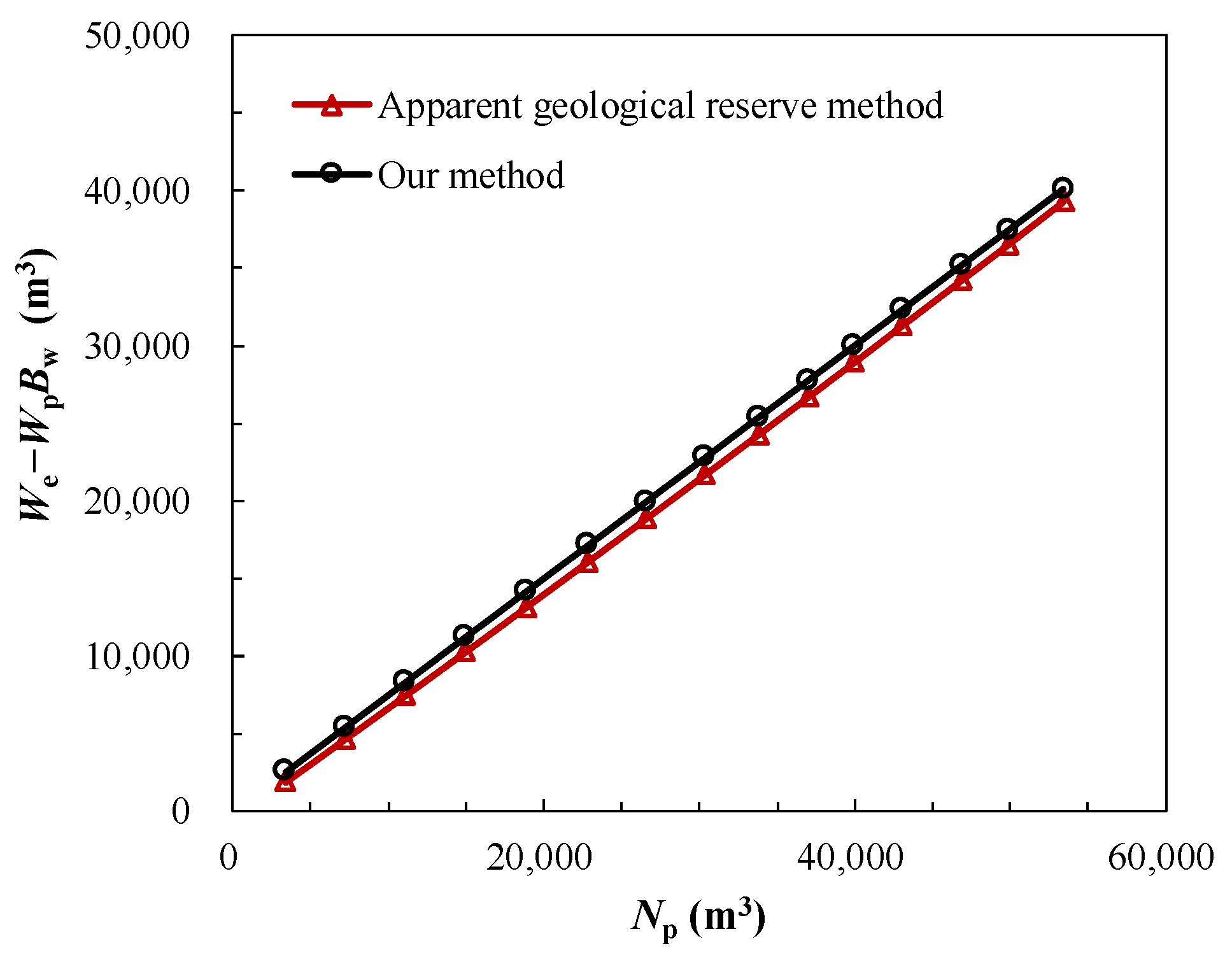
| p (MPa) | Bo Dimensionless | Np (m3) | Wp (m3) | Apparent Geological Reserve Method (We − WpBw) (m3) | Our Method (We − WpBw) (m3) | Relative Discrepancy (%) |
|---|---|---|---|---|---|---|
| 70.82 | 2.567 | 3383.17 | 65.93 | 1868.52 | 2537.38 | 35.80 |
| 70.49 | 2.570 | 7182.86 | 143.28 | 4605.53 | 5387.15 | 16.97 |
| 70.15 | 2.572 | 11,091.32 | 247.27 | 7438.20 | 8318.49 | 11.83 |
| 69.82 | 2.574 | 14,909.24 | 323.10 | 10,222.23 | 11,181.93 | 9.39 |
| 69.47 | 2.576 | 18,864.04 | 396.96 | 13,123.74 | 14,148.03 | 7.80 |
| 69.13 | 2.579 | 22,810.20 | 486.52 | 16,036.85 | 17,107.65 | 6.68 |
| 68.81 | 2.581 | 26,528.77 | 550.13 | 18,798.32 | 19,896.58 | 5.84 |
| 68.47 | 2.583 | 30,343.55 | 600.51 | 21,647.77 | 22,757.66 | 5.13 |
| 68.18 | 2.585 | 33,766.67 | 635.50 | 24,218.92 | 25,325.00 | 4.57 |
| 67.89 | 2.587 | 36,996.19 | 673.29 | 26,657.00 | 27,747.14 | 4.09 |
| 67.64 | 2.588 | 39,949.24 | 702.11 | 28,896.87 | 29,961.93 | 3.69 |
| 67.37 | 2.590 | 43,033.64 | 732.16 | 31,247.07 | 32,275.23 | 3.29 |
| 67.03 | 2.592 | 46,869.24 | 783.10 | 34,184.92 | 35,151.93 | 2.83 |
| 66.77 | 2.594 | 49,871.80 | 826.23 | 36,496.51 | 37,403.85 | 2.49 |
| 66.46 | 2.596 | 53,431.04 | 896.08 | 39,250.11 | 40,073.28 | 2.10 |
| Parameter | Value | Unit | Parameter | Value | Unit |
|---|---|---|---|---|---|
| psc | 0.101325 | MPa | Boi | 2.463 | |
| Tsc | 293 | K | Bw | 1.0344 | |
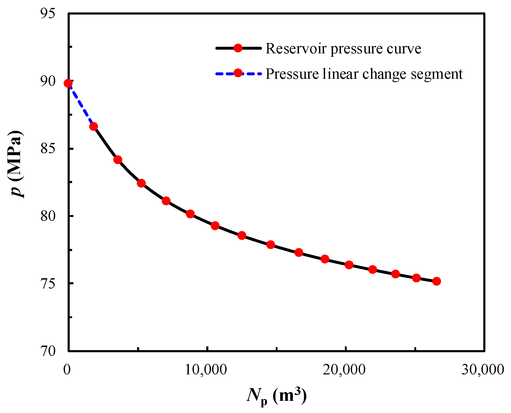
| pi | 89.8 | MPa | Cw | 0.00045 | MPa−1 |
| T | 423.48 | K | Cf | 0.0001 | MPa−1 |
| ρo | 0.8 × 10³ | kg/m3 | Swi | 0 |
| Date | Cumulative Days of Production (d) | Np (m3) | Wp (m3) | p (MPa) |
|---|---|---|---|---|
| 15 September 2021 | 0 | 0 | 0 | 89.80 |
| 10 October 2021 | 25 | 1805.37 | 46.32 | 86.58 |
| 27 December 2021 | 50 | 3551.65 | 77.52 | 84.13 |
| 21 January 2022 | 75 | 5267.72 | 120.35 | 82.40 |
| 15 February 2022 | 100 | 7039.40 | 134.75 | 81.10 |
| 12 March 2022 | 125 | 8781.00 | 150.71 | 80.11 |
| 11 April 2022 | 150 | 10,599.23 | 166.06 | 79.27 |
| 15 May 2022 | 175 | 12,534.98 | 181.32 | 78.52 |
| 9 June 2022 | 200 | 14,598.91 | 214.4 | 77.83 |
| 4 July 2022 | 225 | 16,617.45 | 241.31 | 77.25 |
| 29 July 2022 | 250 | 18,478.59 | 278.89 | 76.78 |
| 23 August 2022 | 275 | 20,234.52 | 308.94 | 76.37 |
| 17 September 2022 | 300 | 21,937.77 | 344.84 | 76.01 |
| 12 October 2022 | 325 | 23,607.90 | 366.08 | 75.68 |
| 21 November 2022 | 350 | 25,123.31 | 400.86 | 75.40 |
| 16 December 2022 | 375 | 26,555.01 | 424.23 | 75.16 |
Disclaimer/Publisher’s Note: The statements, opinions and data contained in all publications are solely those of the individual author(s) and contributor(s) and not of MDPI and/or the editor(s). MDPI and/or the editor(s) disclaim responsibility for any injury to people or property resulting from any ideas, methods, instructions or products referred to in the content. |
© 2024 by the authors. Licensee MDPI, Basel, Switzerland. This article is an open access article distributed under the terms and conditions of the Creative Commons Attribution (CC BY) license (https://creativecommons.org/licenses/by/4.0/).
Share and Cite
Yao, C.; Yan, R.; Zhou, F.; Zhang, Q.; Niu, G.; Chen, F.; Cao, W.; Wang, J. A Novel Method to Calculate Water Influx Parameters and Geologic Reserves for Fractured-Vuggy Reservoirs with Bottom/Edge Water. Energies 2024, 17, 2822. https://doi.org/10.3390/en17122822
Yao C, Yan R, Zhou F, Zhang Q, Niu G, Chen F, Cao W, Wang J. A Novel Method to Calculate Water Influx Parameters and Geologic Reserves for Fractured-Vuggy Reservoirs with Bottom/Edge Water. Energies. 2024; 17(12):2822. https://doi.org/10.3390/en17122822
Chicago/Turabian StyleYao, Chao, Ruofan Yan, Fei Zhou, Qi Zhang, Ge Niu, Fangfang Chen, Wen Cao, and Jing Wang. 2024. "A Novel Method to Calculate Water Influx Parameters and Geologic Reserves for Fractured-Vuggy Reservoirs with Bottom/Edge Water" Energies 17, no. 12: 2822. https://doi.org/10.3390/en17122822