Constructing Australian Residential Electricity Load Profile for Supporting Future Network Studies

Abstract

This paper examines how Australian residential load profiles may evolve in the short to medium term future. These profiles can be used to support simulation studies of the future Australian network within an environment that is transitioning to renewable energy and broader use of electricity as a tool for decarbonisation. The daily profiles rely heavily on the Australian Energy Market Operator (AEMO) forecasts for future annual energy usage. The period from 2024 to 2050 will be transformational. In the residential networks, two secular trends are particularly important in expanding residential generation and electrification. New daily load profiles have been constructed using historical Australian profiles and adding additional components for solar generation, battery operation and electrification activities. The entire aggregated residential network is expected to have reverse midday power flow on any average day from 2024 onwards due to the rapid increase in electric vehicle (EV) usage. The domestic energy demand forecasting methodology presented in this work related to Australia can easily be adopted to carry out similar forecasting for any country of the world.

1. Introduction

The load profiles are used within simulation studies to assess the performance of a network or to assess the impact of an item of equipment. The type of load profile required is determined by the objective of the simulation study. A key assessment of network performance is the voltage profile under peak load conditions. Historical recordings of load profile were examined, often using statistical methods to account for load diversity, to determine a representative measure of likely maximum customer demand. This measure is frequently referred to as “after diversity maximum demand” (ADMD) [1,2,3]. The load recordings were made at an MV distribution feeder or distribution transformer level. These group recordings naturally include the load diversity effect. Load diversity is a critical design factor that is advantageously and directly captured by this approach [4,5]. In historical settings, prior to the widespread application of roof top solar systems, networks were assessed with each connected customer modelled as an ADMD load to determine if the voltage profile met the statuary requirements. For LV network design, the load profile was reduced to a single load value. This diversity-based analysis is simple and well suited to older and limited computing environments that run load flow analysis. The ADMD approach produces reliable results in a system where there is exactly one critical loading scenario. The approach fails if a significant amount of embedded generation is introduced [6]. Australia is committed to achieve net zero emission by 2050 stated in the 2022 Annual Climate Statement under Paris Agreement [7]. Residential solar generation is forecast to increase from 18.7 TWh in 2024 to 63.7 TWh in 2050. Averaged at the household level, daily generation rises from 5.3 kWh to 12.8 kWh. Residential battery installations will grow from 4.2 GWh to 24.2 GWh. At the household level, the average battery size grows from 0.43 kWh to 1.77 kWh [8]. Electrification is the conversion of activities that rely on fossil fuels to electrical alternatives. The conversion of light duty vehicles to electricity dominates in the residential sector with EV charging requiring 35.36 TWh, or 7.07 kWh per household, in 2050. The average number of EVs per household rises from 0.015 in 2024 to 1.05 in 2050. In 2050, this represents 24 million EVs in 13.7 M residences [9]. The other key factor is electrification activities, i.e., conversion of water heating, space heating and cooking appliances from gas to electricity. By 2050, the additional demand from electrification is 13.7 TWh [10]. Total or gross residential consumption across the forecast period rises from 57.04 TWh in 2024 to 107.5 TWh in 2050. At the consumer level, daily consumption rises from 16.1 kWh to 21.6 kWh. The 50.1 TWh rise in consumption is largely offset by a 34.1 TWh increase in residential solar generation. In 2024 the distribution networks will supply 9.6 M consumers with 38.3 TWh, or an average of 10.8 kWh daily. In 2050, they are forecast to supply 43.8 TWh to 13.7 million customers, with an average daily supply of 8.8 kWh. The number of consumers grows but the energy served each day is static [11].

Considering the above figures for PV, storage and electrification, at least two critical scenarios emerge: the traditional peak load scenario and the peak generation or low demand scenario [12]. Arguably, the single case ADMD based design approach can be easily extended to include a second scenario. This can be a minimum load case, and this becomes important for MV network design, and the development of a transformer tap setting plan. Another approach to extracting the load profile is to use a time series solution, where each customer has a time varying load and generation behaviour [13,14]. A time-based solution will use a consumer load profile with a specified sampling time. It can use historically recorded data or synthesised data. Historical data can be collected from consumers with dedicated recorders or using a smart meter infrastructure. Synthetic load profiles can be produced by using historical data utilising the knowledge of customer behaviour and appliance usage [15,16]. A stochastic bottom-up approach is adapted to model flexible load profiles considering user behaviour in [17]. The authors have presented a bottom-up model by using household appliances usage [18]. This paper also uses a bottom-up approach to model the residential load profiles for the Australian distribution network. New daily load profiles have been constructed using historical Australian profiles and adding additional components for solar generation, battery operation and electrification activities. The main contribution of the paper is to develop Australian residential load profiles covering the period 2024 to 2050. The profiles can be used within electrical distribution network simulation and modelling studies to support the sustainable growth of renewable energy generation. The methodology can be used to forecast the load profiles for any other region with similar datasets.

2. Methodology

In this paper, a bottom-up approach is used to construct the residential load profile for the years 2024, 2030, 2040 and 2050. Figure 1 shows the diagram of the bottom-up approach. To perform the load forecasting, several energy components are considered: (1) solar (Es); (2) electric vehicles (Eev); (3) energy storage (Ees); (4) electrification (Ee); (5) underlying consumption (Ec). The load profiles for each energy component are constructed using their respective models M1 to M5 from relevant datasets at a particular time (t), discussed in the following sections. Then, they are added to predict the net load profile.

3. Factoring Load Growth

The most recent energy forecasts details and numerical data can be downloaded from the AEMO forecasting web portal [19].

Table 1. AEMO Annual Energy Consumption Central Forecast (TWh).

Energy Component	2024	2030	2040	2050
Roof top PV—total	23.1	39	62.5	86.9
Residential	18.7	31.1	48.7	63.7
Business	4.4	7.3	13.8	23.2
Electric vehicles—total	0.287	5.38	20.68	35.36
Residential (68%)	0.277	4.48	16.95	28.88
Light Commercial Vehicle (LCV) (38%)	0.01	0.904	3.73	6.49
Electrification	1.29	16.97	33.3	41.2
Residential	0.03	3.07	8.5	13.7
Business	1.26	13.9	24.8	27.5
AEMO Residential demand	36.6	25.9	10.7	−4.1
Corrections to residential demand
Small non-scheduled generation (SNSG) offset	1.6	2.3	3.1	4.6
Electrification	0.03	3.07	8.5	13.7
Electric vehicles	0.11	3.03	15.9	29.6
Roof top PV supply to homes	18.7	31.1	48.7	63.7
Total correction	20.44	39.5	76.2	111.6
Underlying residential demand	57.04 TWh	65.4 TWh	87.9 TWh	107.5 TWh
Number of residential National NMIs	9,698,322	10,600,406	12,135,686	13,657,214
Underlying Consumption per NMI
Annually	5.88 MWh	6.16 MWh	7.24 MWh	7.87 MWh
Daily	16.1 kWh	16.9 kWh	19.8 kWh	21.6 kWh
Solar generation per NMI
Annually	1.93 MWh	2.93 MWh	4.01 MWh	4.66 MWh
Daily	5.3 kWh	8.03 kWh	10.9 kWh	12.8 kWh
Net Consumption per NMI
Annually	3.95 MWh	3.23 MWh	3.23 MWh	3.21 MWh
Daily	10.8 kWh	8.87 kWh	8.9 kWh	8.8 kWh
EV Charging per NMI
Annually	0.029 MWh	0.509 MWh	1.704 MWh	2.58 MWh
Daily	0.081 kWh	1.39 kWh	4.67 kWh	7.07 kWh
Equivalent vehicles per NMI	0.015	0.22	0.69	1.05
Electrification per NMI
Annually	0.003 MWh	0.29 MWh	0.7 MWh	1 MWh
Daily	0.009 kWh	0.79 kWh	1.9 kWh	2.74 kWh

contains numerical information extracted from the Electricity Statement of Opportunities (ESOO) online web portal. The ESOO separates future load growth into specific components. To estimate the residential gross demand, i.e., the demand behind the meter, several components must be considered. Solar energy is separated into residential and business components. The residential PV component must be added to the observed residential demand to determine the gross, or the behind the meter, energy demand. Electrification is again separated into a residential and business component. The residential component adds to the residential gross demand. Electric vehicle growth is separately identified. The online portal does not separate residential and business use. Finally, in the portal data downloads, AEMO includes a correction for “Small non-scheduled generation” (SNSG). Table 1 shows a strong growth in residential energy consumption. At the customer level, demand grows from 5.88 MWh to 7.87 MWh annually in 2050. The growth in energy demand of 1.99 MWh is offset by solar growth. Average solar generation increases by 2.73 MWh from 1.93 MWh to 4.66 MWh annually. The load increase is, within the tolerances of this exercise, balanced by the increased solar generation.

3.1. The Solar Load Profile

PVWatts is a PV forecasting tool provided by NREL. Generation profiles can be produced at any selected geographical location using local meteorological data. Several years of local data are used to generate a statistically representative year. Figure 2 shows the AC power output from a 1 kWp array, north facing with an inclination of 20° at Brisbane during the summertime from 1 December to 28 February representing different colors. Data was sourced from the Brisbane Bureau of Meteorology (BoM).

The top trace shows 90 days of summertime generation. On ideal days, a 1 kWp array produces approximately 800 W at the AC terminals. The average generation profile is shown below. The average peaks at 595 W.

Table 2. Average summer generation at Brisbane.

Time	Generation from 1 kWp (W)	1 kWh/day Generation Profile (W)
00:00:00	0.0	0.0
01:00:00	0.0	0.0
02:00:00	0.0	0.0
03:00:00	0.0	0.0
04:00:00	0.0	0.0
05:00:00	12.1	2.6
06:00:00	90.5	19.5
07:00:00	243.2	52.3
08:00:00	396.4	85.3
09:00:00	517.5	111.4
10:00:00	546.0	117.5
11:00:00	578.9	124.6
12:00:00	594.7	128.0
13:00:00	549.5	118.3
14:00:00	470.6	101.3
15:00:00	366.8	79.0
16:00:00	209.3	45.1
17:00:00	66.5	14.3
18:00:00	3.5	0.8
19:00:00	0.0	0.0
20:00:00	0.0	0.0
21:00:00	0.0	0.0
22:00:00	0.0	0.0
23:00:00	0.0	0.0
Total	4645.4 Wh	1000.0 Wh

contains the hourly power outputs. The average daily energy produced is 4645 Wh. Table 2, column 3, contains hourly generation figures for an array producing an average daily energy yield of 1 kWh. These figures can be used to scale a solar generation profile that yields a specific average amount of energy.

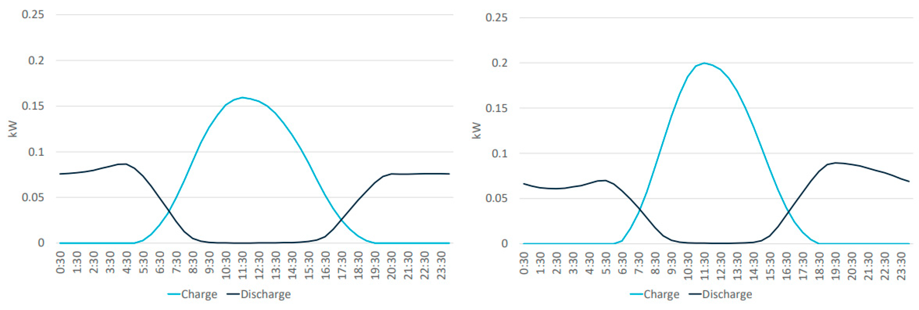
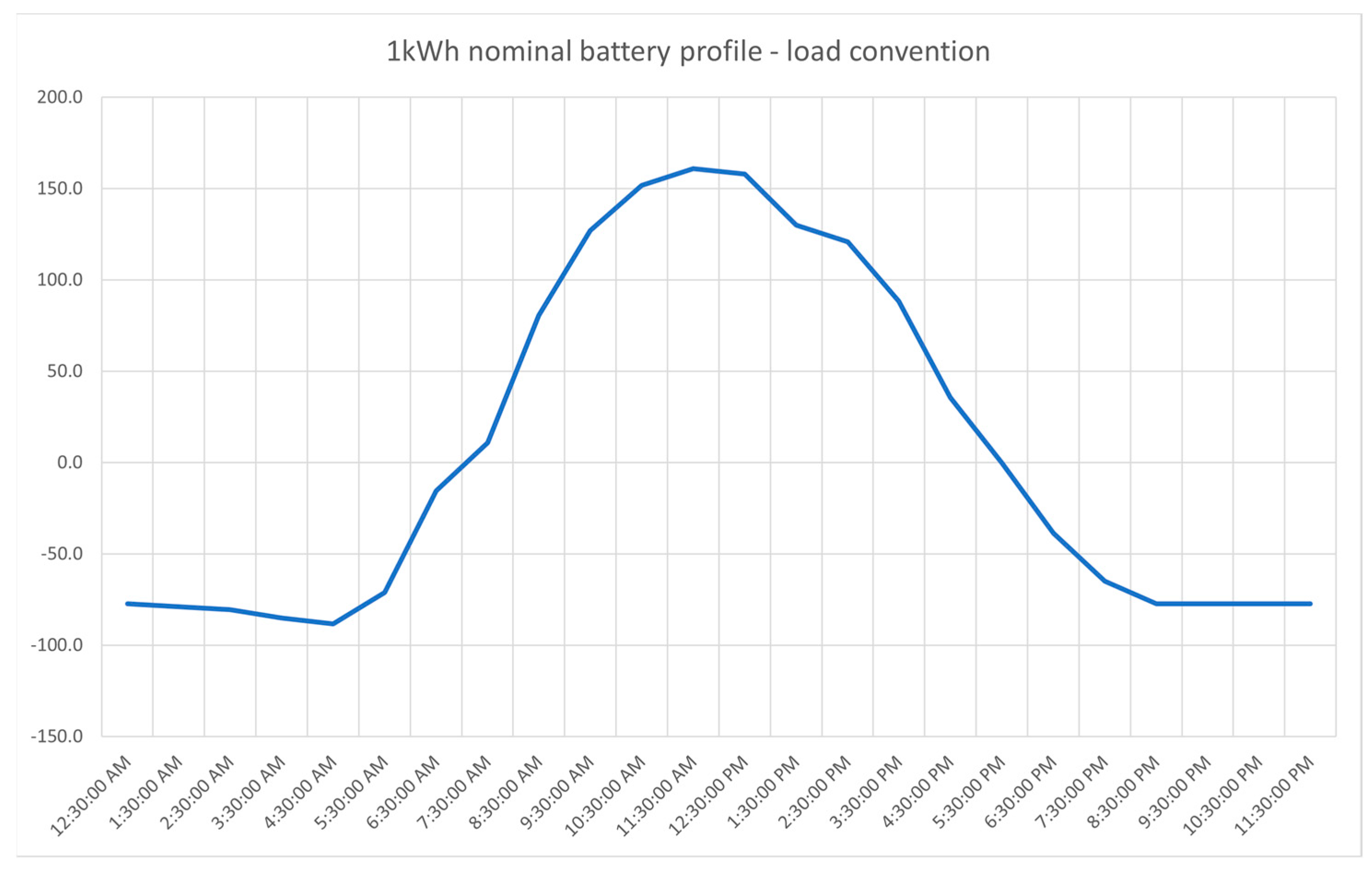
3.2. Residential Energy Storage Profile

AEMO has forecast small scale energy storage battery installations per customer, which is shown in

Table 3. Cumulative battery capacity degraded GWh.

Year	Installed Capacity (GWh)	NMI Number	Capacity per Customer
2024	4.2	9,698,322	0.43 kWh
2030	11.5	10,600,406	1.08 kWh
2040	17.8	12,135,686	1.47 kWh
2050	24.2	13,657,214	1.77 kWh

[8]. The battery can be managed in a variety of ways. For a residential tariff connection, the most frequent controls aim to maximise self-consumption. A consumption curve suitable for maximising self-consumption is shown in Figure 3 [8]. The curves are normalised curves for a battery with a discharge capacity of 1 kWh. The battery charging power is proportional to the expected solar power. This approach ensures that the battery capacity is spread across the day. The net battery power shown in Figure 4 can be calculated from Equation (1).

$$P_{b,net}=P_{b,ch}-P_{b,dis}$$

(1)

where, $P_{b,net}$ = Net battery power, $P_{b,ch}$ = Charging power, and $P_{b,dis}$ = Discharging power.

The charging and discharging power can be found from the summer profile curve of Figure 3. This is normalised to a 1 kWh discharge rating.

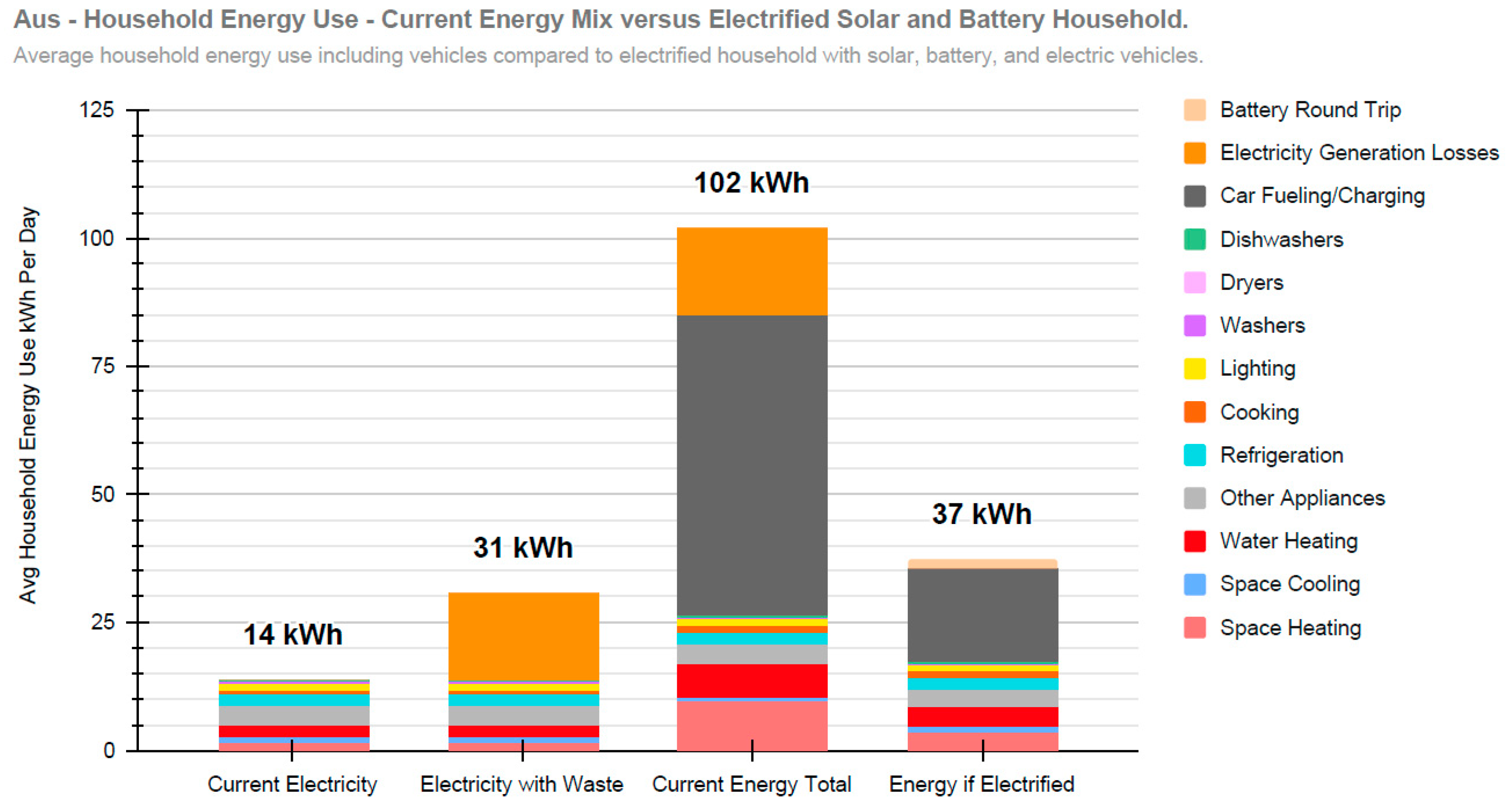
3.3. Electrification

Electrification offers significant benefits for space heating. Heat pumps for heating and cooling transfer more heat than electrical input. A residential heat pump with a typical coefficient of performance (CoP) of 4, for example, will produce a heating effect of 4 kW with an electrical input of 1 kW. Figure 5 shows an estimate of the energy flows in a typical Australian home [20]. The first column suggests the annual residential consumption is 14 kWh/day. This is close to the AEMO consumption in 2024 of 16.1 kWh/NMI. The second column shows the energy input to the generation sources, 31 kWh, to deliver 14 kWh to a residential consumer. The third column shows all the inputs to a typical household. Fuel for vehicles is the single largest energy input. However, there is also a considerable fossil fuel input, mostly gas, for water or space heating. The fourth column shows the electrical requirement, 37 kWh, if all fossil fueled processes are converted to electric equivalents. In the fully electrified home electrical energy for water and space heating has increased by 3 kWh from approximately 4 kWh to 7 kWh. In comparison, cooking is a smaller energy component. The electrification process increases from roughly 1 kWh/day to 2 kWh/day. The AEMO energy forecasts, shown in Table 1, suggest that by 2050 electrification results in an additional 2.74 kWh of consumer load. This suggests that electricity has taken most of the heating and cooling burden by 2050.

Several factors will affect the load profile for electrification, namely:

• Water heating, either by resistance heating or heat pump, will mostly use hot water storage. Existing practice shows water heating load is readily deferrable.
• Space heating is partially deferrable and improves with a longer building thermal time constant.
• Cooking is not deferrable but smaller in energy terms.

Efficient thermal storage requires that the thermal system time constant is longer than the storage time. Hot water services have time constants measured in days. For a few hours of storage, the efficiency is comparable to battery systems. Hot water systems are a high-quality deferrable load asset that can be easily moved to adjust the load profile. Cooking, in terms of contrast, is strongly associated with mealtimes and contributes to a morning and evening peak.

In regions where heating is important, such as Victoria, the existing homes have a thermal time constant measured in hours. Across Australia, building regulations impose an energy star rating system [21,22] for new construction. The star rating systems always include high insulation requirements. This increases thermal resistance to ambient. If the internal thermal mass remains, the same the thermal time constant increases. The star rating of Australia’s residential buildings, and the thermal time constant, is improving over time. The replacement cycle for buildings is more than 50 years. The 2050 housing stock will still contain many dwellings with lower star ratings.

In a building with a time constant of just a few hours, the space heating demand must approximately follow the temperature differential between the interior and the ambient. The existing Australian housing stock falls into this category. Heating will start in the evening and continue until the occupants go to bed. Heating will contribute to the evening peak. If the internal temperature is allowed to drop overnight, it is likely that morning heating will be used contributing to a morning peak. Many networks in the southern parts of Australia have a dominant morning peak in winter.

In a building with a very high thermal resistance and thermal time constant of tens of hours, the heat energy input can occur at any point in the 24-h cycle. The heating system power can be small if the energy input is applied over many hours each day. The heat input can be tailored to optimise the load profile. Buildings of this type are common in the northern parts of Europe and America. The insulation systems have thermal resistances that are an order of magnitude above those applied in Australia. In some cases, the waste heat from appliances and the occupants provides most of the space heating input.

The features of electrification load profile selected for this study will be:

• A morning and evening peak caused by space heating and cooking.
• Water heating contributes to load at off-peak times.

The residential existing demand profiles have the same generalised shape. In the absence of better modelling information, it is recommended that the electrification load be modelled with the same load shape as the existing consumer demand.

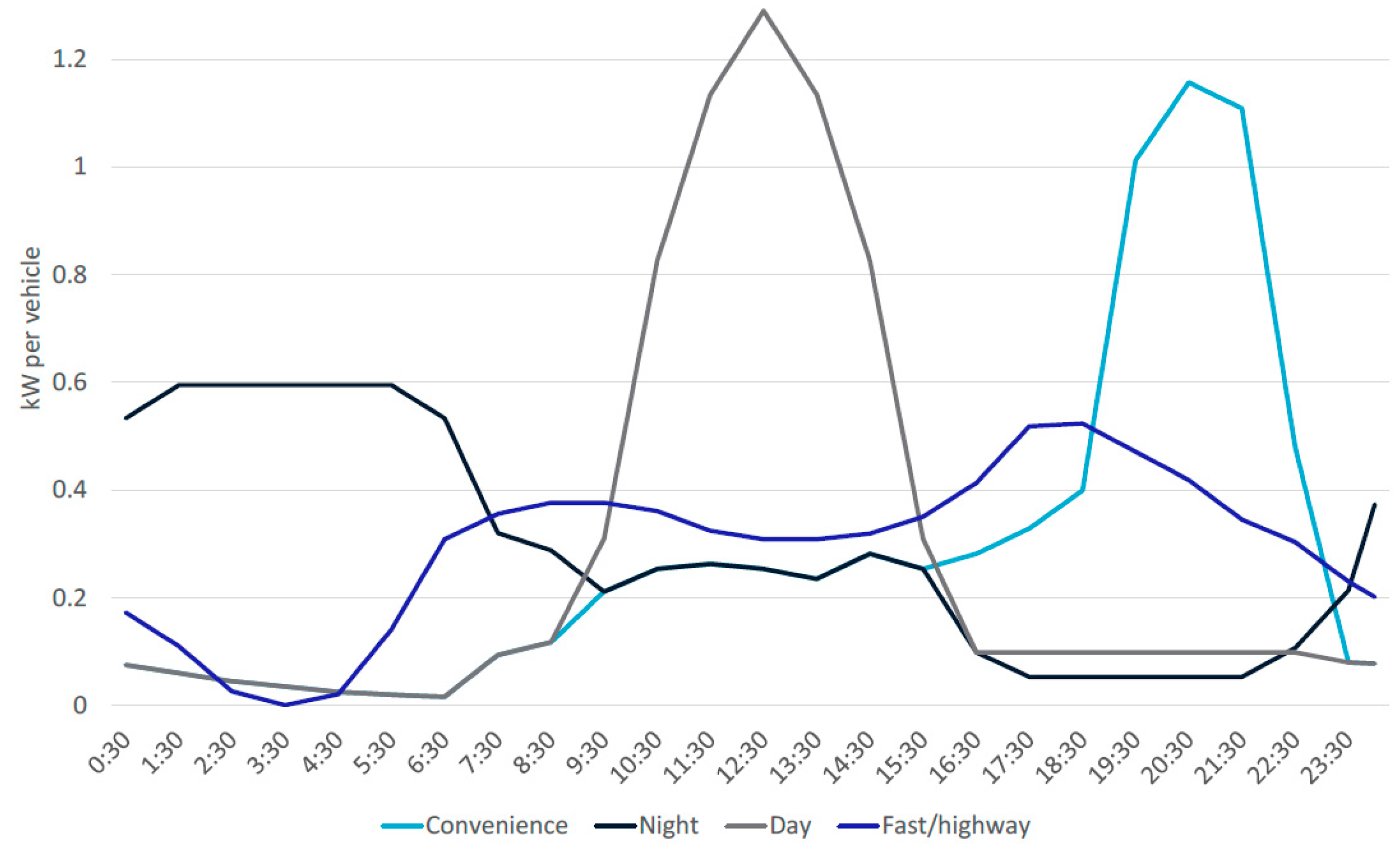
3.4. Electric Vehicle Profile

Australian homes generally have garages, and the on-street parking of private cars is less frequent. Residential charging is normally performed with AC power from a general-purpose outlet (GPO) or from a dedicated wall charger. The vehicle typically has an on-board battery charger. Charging can be single phase or three phase. Many, and perhaps most, Australian households will charge vehicles with either 10 A or 16 A GPOs. Some households will opt to install a wall charger, which is typically:

• 32 A single phase or 7 kW
• 16 A to 32 A three phase, which is 11–22 kW.

As of the 31 January 2021, Australia had 20.1 million vehicles with an average age of 10.6 years [23]. In 2023, a total of 87,217 electric passenger vehicles were registered. This was an increase of 261% on the previous year’s sales of 33,410 vehicles in 2022. The Commonwealth Scientific and Industrial Research Organization (CSIRO) has adopted after-diversity daily charging profiles for light vehicles shown in Figure 6 [24]. This paper adopts this level of energy consumption for year 2024 and year 2030. The CSIRO report has relied on older reference materials with publication dates from 2013 to 2016. The recent overseas experience shows that off-peak and super off-peak charging is popular [25]. This article reported on the behaviours of 1689 EV customers with a breakup as follows:

• IBT EV consumers 876: IBT EV consumers staying with base rate—549, IBT EV consumers switching to EV rate—327.
• TOU EV consumers 813: TOU EV consumers staying with base rate-399, TOU EV consumers switching to EV rate—414.

Of the 1689 EV owners, 741 (44%) switched to an EV super off-peak rate while 399 (24%) were on a generic time of use tariff. Some 1140 owners are on TOU tariffs. As a proportion, this is 67%. The CSIRO report suggests the public charging share is 11% with 89% of charging occurring at home. This is consistent with the recent literature. This paper recommends that 67% of the home charging, or 60% of the total charging, is controlled in some way. If the V2G share remains at 12%, then night charging should be 48%. The resulting break up of charging profiles is as follows:

• Home convenience charging 29%
• Home night charging 48%
• Home V2G charging 12%
• Public charging fast charge highway 5%
• Public charging solar aligned 6%.
• This paper has used the profile shown in Figure 6 to develop the net EV profile for years 2024 and 2030. The equation is expressed as follows:

$$P_{ev,net}=P_{ev}\left(nightcharging60\%\right)+P_{ev}\left(conviniencecharging29\%\right)$$

(2)

The resulting profile for a residentially charged EV is shown in Figure 7. This profile has been used to develop year 2024 and year 2030 profiles. However, CSIRO has published charging profiles for light vehicles in 2035 and 2050, which have been used to develop the profiles for 2040 and 2050 [9]. Light vehicles include 68% home charging and CSIRO has also considered light commercial vehicles (LCV), which will use 38% home charging.

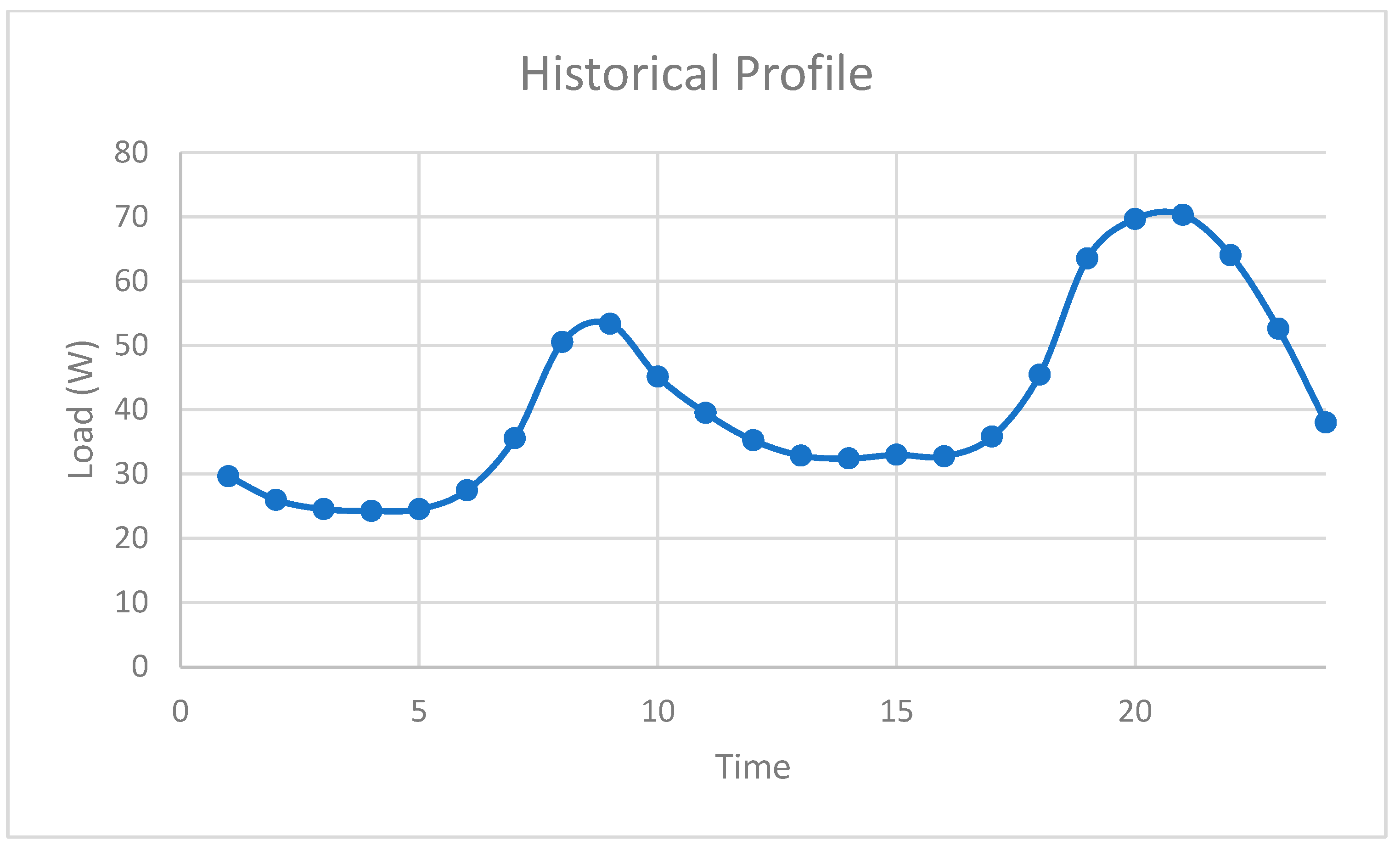
3.5. Underlying Consumption Profile

This article has adopted the load profile from AEMO [26] that has been synthesised from the Ausgrid data set, which is shown in Figure 8. Privacy considerations limit access to consumer data. This profile is aggregated by using the historical dataset of [27] to construct the real profile.

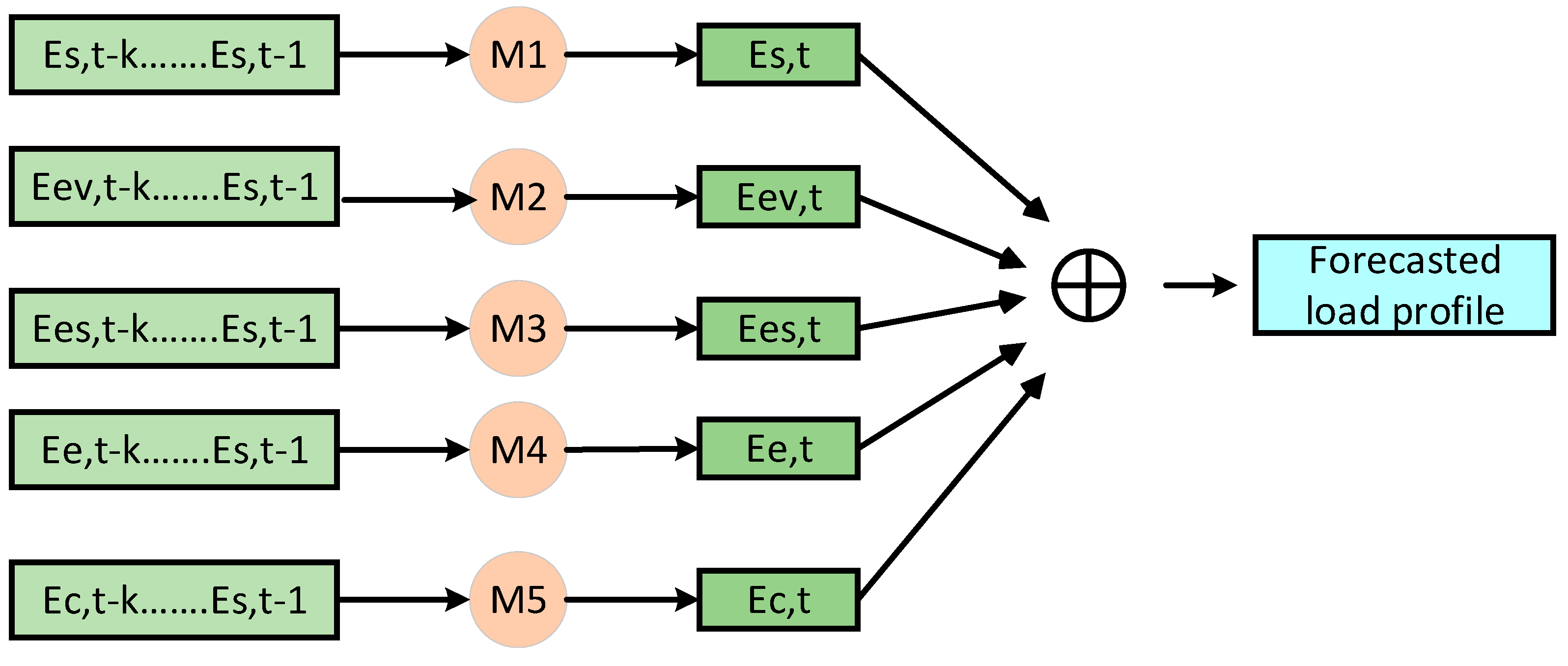
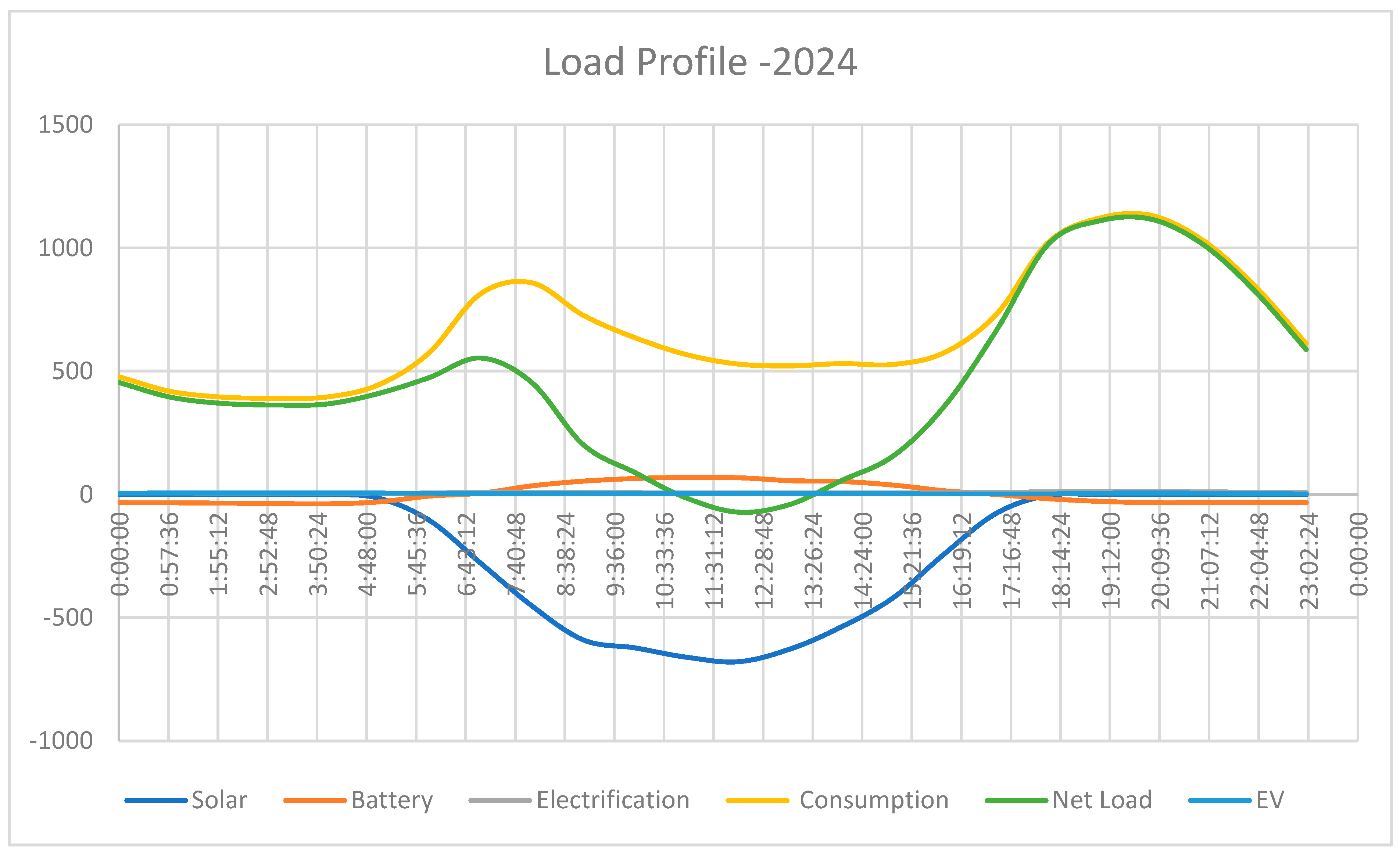
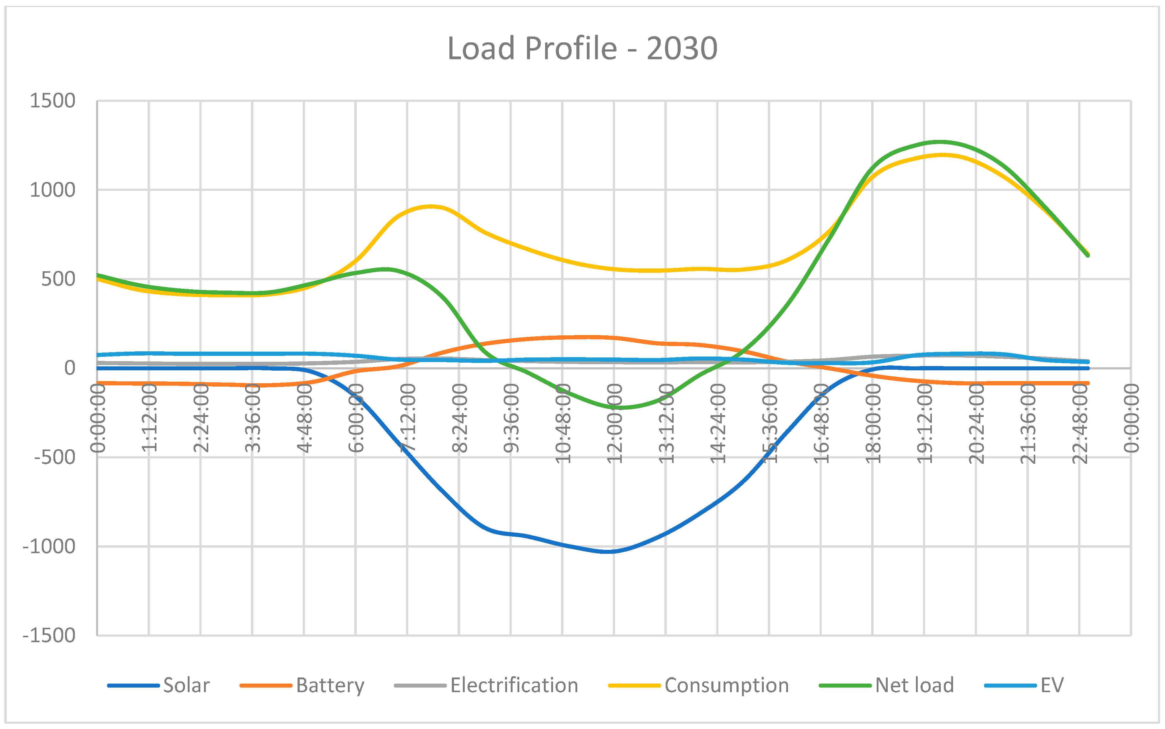
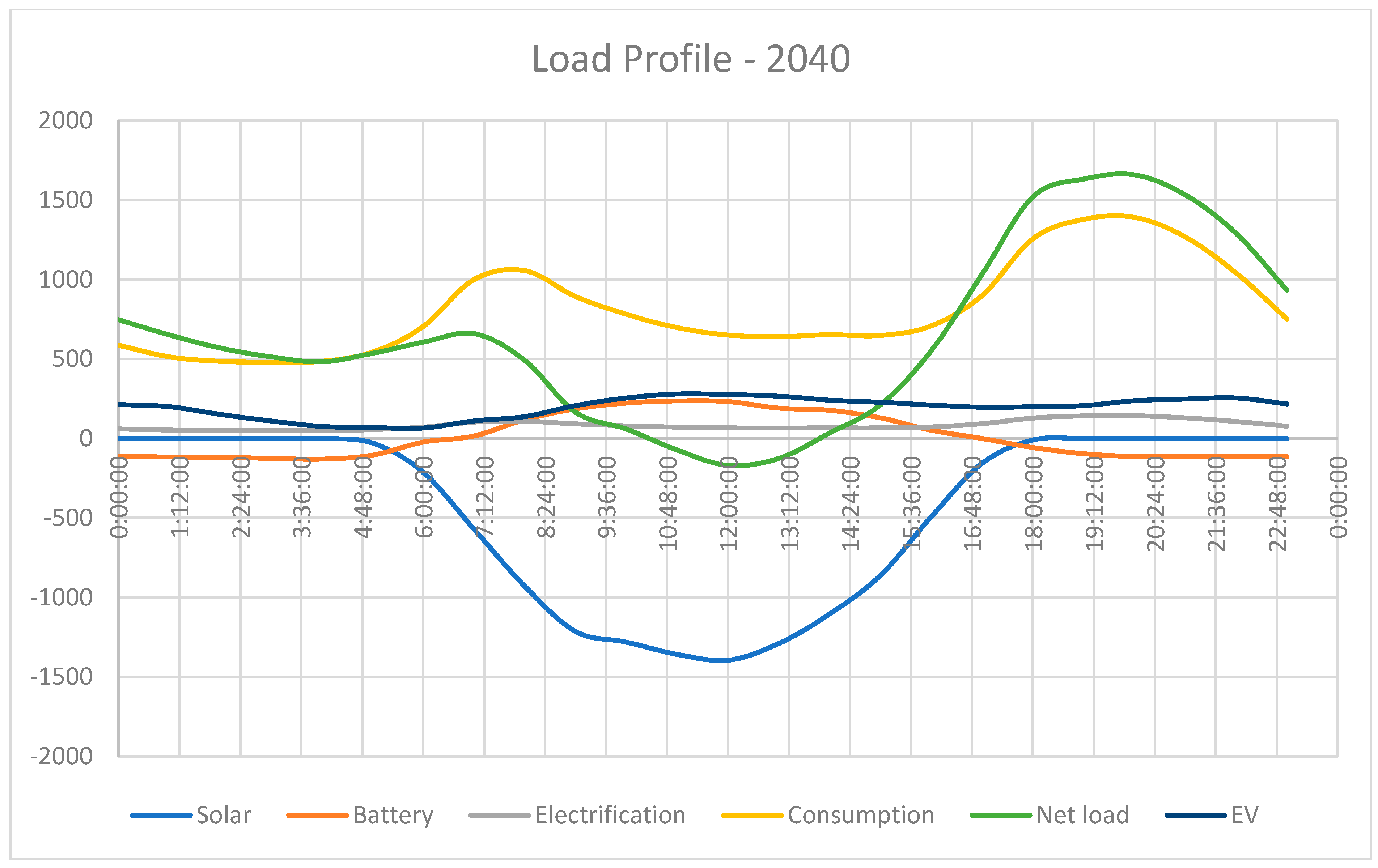
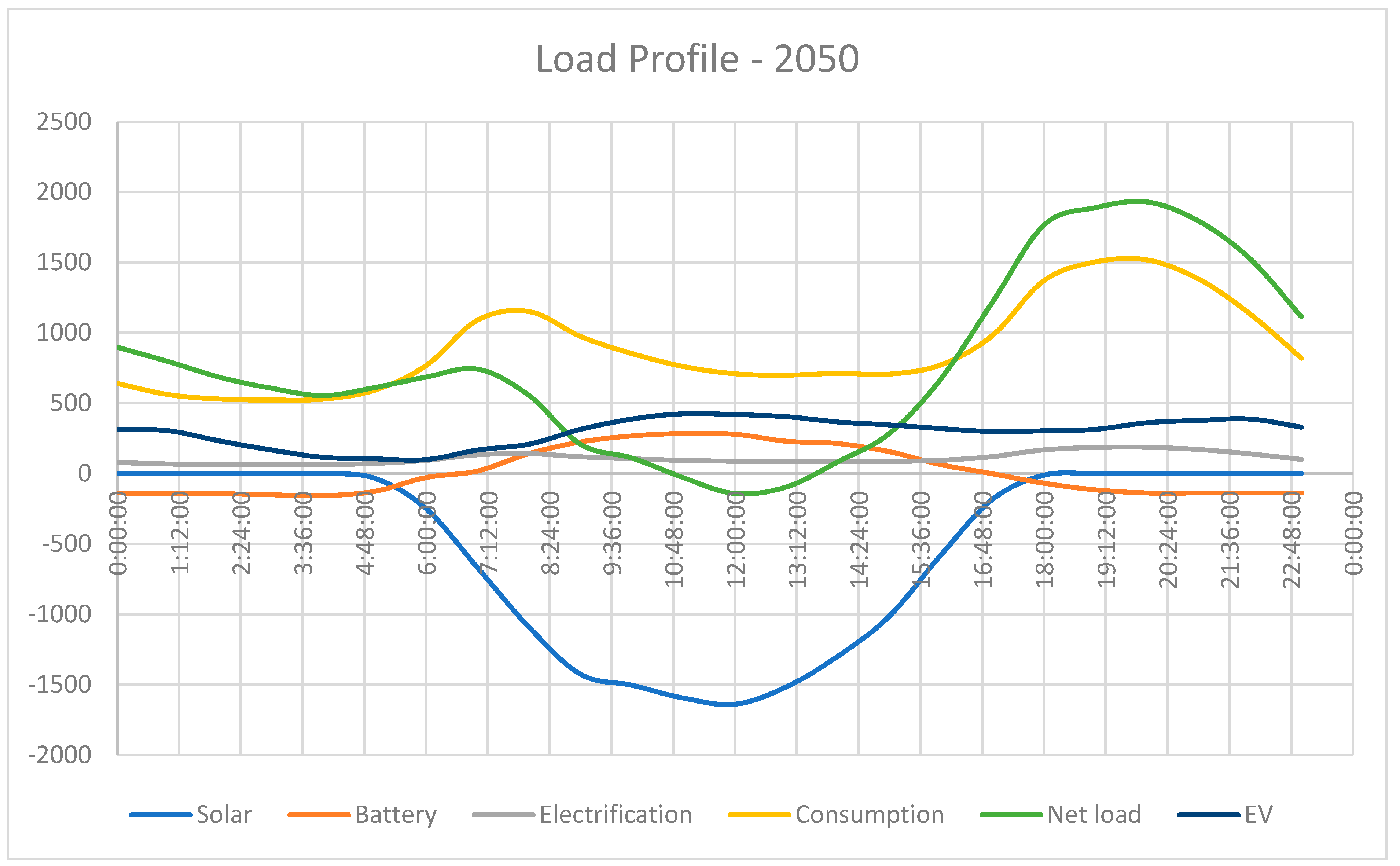
4. Modelling Load Profiles

The forecast profiles are constructed using the energy components listed in Table 2 along with the device load profiles developed above. The equation used to construct the profile is given below:

$${Forecastedprofile}_{x,y}={\sum }_{t=0}^{23}{GrowthperNMI}_y\ast {Loadprofile}_{x,y}$$

(3)

where $x$ = each component, such as solar, battery, electrification etc. $y$ = Year.

The profiles and underlying components are plotted in Figure 9, Figure 10, Figure 11 and Figure 12.

5. Insights into Constructed Profiles

Table 4. Average load profile metrics over time.

Parameter	2024	2030	2040	2050
Net energy per NMI	10.9 kWh	11.2 kWh	15.5 kWh	18.5 kWh
Solar generation per NMI	5.3 kWh	8.03 kWh	10.9 kWh	12.8 kWh
Gross Energy per NMI	16.2 kWh	19.23 kWh	26.4 kWh	31.3 kWh
Maximum demand	1116 W	1257 W	1659 W	1930 W
Minimum demand	−71 W	−219 W	−169 W	−140 W

shows some key load profile metrics for each year. The profiles presented in the above section are on a customer basis. The number of NMIs increases from 9.6 million in 2024 to 13.7 million in 2050, an increase of 43%.

The gross energy consumption per customer rises over the forecast period from 16.2 kWh to 31.3 kWh in 2050. Most of this increase in gross consumption is provided by solar generation. Solar generation, per NMI, increases from an average of 5.3 kWh to 12.8 kWh over the forecast period. As a result, the energy served per customer is relatively static. The net customer energy in 2024 is 10.9 kWh and this rises by 69.7% to 18.5 kWh in 2050. The total energy served in the distribution network will be more strongly affected by the growth in consumer numbers. The average peak demand increases by 73% over the forecast period from 1116 W to 1930 W in 2050. The minimum load, −71 W in 2024, becomes negative from 2024 onwards. The largest negative minimum load is −219 W in 2030.

It is worthwhile pointing out that this is a national energy market (NEM) wide average. The implication is that, on any given day, it is likely that the entire residential load reverses. This report does not examine business and commercial loads. These sectors will invest heavily in solar energy. The growth rates in this area are likely to exceed the growth rates for residential systems as this market is maturing. There is no guarantee that business loads will be a willing sink for reverse flows from the residential customers.

The 2050 household will have significant load demand management opportunities. The periods of negative demand might be addressed if appropriate incentives exist.

6. Conclusions

This paper proposed Australian residential load profiles covering the period 2024 to 2050. Residential solar generation is forecast to increase from 18.7 TWh in 2024 to 63.7 TWh in 2050. At the household level, daily generation rises from 5.3 kWh to 12.8 kWh. Residential battery installations will grow from 4.2 GWh to 24.2 GWh. At the household level, the average battery sizes grow from 0.43 kWh to 1.77 kWh.

EV charging will require 7.07 kWh per household in 2050. Studies based on the physical behaviour of EV owners show that off-peak charging is popular. The report departs from AEMO’s recommendation to provide a profile based on more recent published studies.

The report examines other key electrification activities. These are the conversion of water heating, space heating and cooking appliances from gas to electricity. By 2050, the additional demand from electrification is 13.7 TWh.

New daily load profiles have been constructed using historical Australian profiles and adding additional components for solar generation, battery operation and electrification activities. The average peak demand grows modestly from 1116 W in 2024 to 1930 W in 2050. In contrast, the minimum demand, initially recorded at −71 W in 2024, will further decrease to −169 W by 2040 due to the expansion of EV loads and increased battery capacities, ultimately standing at −140 W in 2050. This result carries significant implications as, from 2024 onwards, the entire aggregated residential network is projected to experience reverse power flow on an average day.

References

1. Hernando-Gil, I.; Li, F.; Collin, A.; Djokic, S. Development of sub-transmission network equivalents and after-diversity-demand values: Case study of the UK residential sector. In Proceedings of the 2016 18th Mediterranean Electrotechnical Conference (MELECON), Lemesos, Cyprus, 18–20 April 2016; pp. 1–6. [Google Scholar]
2. Pimm, A.J.; Cockerill, T.T.; Taylor, P.G. The potential for peak shaving on low voltage distribution networks using electricity storage. J. Energy Storage 2018, 16, 231–242. [Google Scholar] [CrossRef]
3. Barteczko-Hibbert, C. After Diversity Maximum Demand (ADMD) Report; Report for the ‘Customer-Led Network Revolution’ Project; Durham University: Durham, UK, 2015. [Google Scholar]
4. Mcdaniel, G.; Gabrielle, A. Load diversity-its role in power system utilization. IEEE Trans. Power Appar. Syst. 1965, 84, 626–635. [Google Scholar] [CrossRef]
5. McKenna, R.; Djapic, P.; Weinand, J.; Fichtner, W.; Strbac, G. Assessing the implications of socioeconomic diversity for low carbon technology uptake in electrical distribution networks. Appl. Energy 2018, 210, 856–869. [Google Scholar] [CrossRef]
6. Giasemidis, G.; Haben, S.; Lee, T.; Singleton, C.; Grindrod, P. A genetic algorithm approach for modelling low voltage network demands. Appl. Energy 2017, 203, 463–473. [Google Scholar] [CrossRef]
7. Net Zero. Available online: https://www.dcceew.gov.au/climate-change/emissions-reduction/net-zero (accessed on 2 April 2024).
8. Graham, P.; Mediwaththe, C. Small-Scale Solar PV and Battery Projections 2022. 2022. Available online: https://aemo.com.au/-/media/files/stakeholder_consultation/consultations/nem-consultations/2022/2024-inputs-assumptions-and-scenarios-consultation/supporting-materials-for-2024/csiro-2022-solar-pv-and-battery-projections-report.pdf (accessed on 24 March 2024).
9. Graham, P. Electric Vehicle Projections 2024: Update to the 2022 Projections Report; CSIRO: Canberra, Australia, 2024; Available online: https://aemo.com.au/-/media/files/stakeholder_consultation/consultations/nem-consultations/2024/2024-forecasting-assumptions-update-consultation-page/csiro---2024-electric-vehicle-projections-report.pdf?la=en (accessed on 28 March 2024).
10. Griffith, S.; Ellison, J.; Calisch, S.; Cass, D. Household Electrification: Savings in the Suburbs. 2021. (webflow.com). Available online: https://615a1e5c7bec5c70d6d3f346_Castles and Cars Rewiring Australia Technical Study.pdf (accessed on 28 March 2024).
11. AEMO. 2024 Inputs, Assumptions and Scenarios Report, Australia, 2024. Available online: https://aemo.com.au/-/media/files/major-publications/isp/2024/2024-inputs-assumptions-and-scenarios-report.pdf (accessed on 28 March 2024).
12. Fila, M.; Taylor, G.A.; Hiscock, J.; Irving, M.R.; Lang, P. Flexible voltage control to support distributed generation in distribution networks. In Proceedings of the 2008 43rd International Universities Power Engineering Conference, Padua, Italy, 1–4 September 2008; pp. 1–5. [Google Scholar]
13. Shi, Y.; Yu, T.; Liu, Q.; Zhu, H.; Li, F.; Wu, Y. An approach of electrical load profile analysis based on time series data mining. IEEE Access 2020, 8, 209915–209925. [Google Scholar] [CrossRef]
14. Firoozjaei, M.D.; Kim, M.; Alhadidi, D. Time-series load data analysis for user power profiling. In Proceedings of the 2023 25th International Conference on Advanced Communication Technology (ICACT), Pyeongchang, Republic of Korea, 19–22 February 2023; pp. 382–387. [Google Scholar]
15. Sandhaas, A.; Kim, H.; Hartmann, N. Methodology for generating synthetic load profiles for different industry types. Energies 2022, 15, 3683. [Google Scholar] [CrossRef]
16. Omar, N.; Ariff, M.A.M.; Shah, A.F.I.M.; Mustaza, M.S.A. Estimating synthetic load profile based on student behavior using fuzzy inference system for demand side management application. Turk. J. Electr. Eng. Comput. Sci. 2020, 28, 3193–3207. [Google Scholar]
17. Fischer, D.; Surmann, A.; Biener, W.; Selinger-Lutz, O. From residential electric load profiles to flexibility profiles–A stochastic bottom-up approach. Energy Build. 2020, 224, 110133. [Google Scholar] [CrossRef]
18. Gao, B.; Liu, X.; Zhu, Z. A bottom-up model for household load profile based on the consumption behavior of residents. Energies 2018, 11, 2112. [Google Scholar] [CrossRef]
19. Australian Energy Market Operator (AEMO). National Electricity & Gas Forecasting. 2024. Available online: https://forecasting.aemo.com.au/Electricity/AnnualConsumption/Operational (accessed on 28 March 2024).
20. Griffith, S. Electrify: An Optimist’s Playbook for Our Clean Energy Future; MIT Press: Cambridge, MA, USA, 2022. [Google Scholar]
21. Energy Efficiency Requirements. Available online: https://www.vba.vic.gov.au/consumers/home-renovation-essentials/energy-efficient-requirements (accessed on 28 March 2024).
22. 6-Star Energy Equivalence Rating for Houses and Townhouses. 2015. Available online: https://www.epw.qld.gov.au/__data/assets/pdf_file/0014/5180/6starenergyequivalenceratingforhousesandtownhousesfactsheet.pdf (accessed on 28 March 2024).
23. Motor Vehicle Census, Australia. Bureau of Statistics. Available online: https://www.abs.gov.au/statistics/industry/tourism-and-transport/motor-vehicle-census-australia (accessed on 28 March 2024).
24. Graham, P.; Havas, L. Electric Vehicle Projections 2021; CSIRO: Canberra, Australia, 2021; Available online: https://aemo.com.au/-/media/files/electricity/nem/planning_and_forecasting/inputs-assumptions-methodologies/2021/csiro-ev-forecast-report.pdf (accessed on 28 March 2024).
25. Qiu, Y.L.; Wang, Y.D.; Iseki, H.; Shen, X.; Xing, B.; Zhang, H. Empirical grid impact of in-home electric vehicle charging differs from predictions. Resour. Energy Econ. 2022, 67, 101275. [Google Scholar] [CrossRef]
26. Graham, P.; Havas, L. Projections for Small-Scale Embedded Technologies; CSIRO: Canberra, Australia, 2020. [Google Scholar]
27. Ratnam, E.L.; Weller, S.R.; Kellett, C.M.; Murray, A.T. Residential load and rooftop PV generation: An Australian distribution network dataset. Int. J. Sustain. Energy 2017, 36, 787–806. [Google Scholar] [CrossRef]
Figure 1. Diagram of the bottom-up approach.
Energies 17 02908 g001
Figure 2. Summertime generation ensemble at Brisbane.
Energies 17 02908 g002
Figure 3. Charge discharge curve for solar self-consumption summer (left) and winter (right) [8].
Energies 17 02908 g003
Figure 4. Battery equivalent load power.
Energies 17 02908 g004
Figure 5. Estimated energy use in an Australian Home [20].
Energies 17 02908 g005
Figure 6. CSIRO light vehicle charging profile [24].
Energies 17 02908 g006
Figure 7. EV Residential Profile, 60% Night Charging, 29% Convenience Charging.
Energies 17 02908 g007
Figure 8. Historical profile.
Energies 17 02908 g008
Figure 9. Load Profile—Year 2024.
Energies 17 02908 g009
Figure 10. Load Profile—Year 2030.
Energies 17 02908 g010
Figure 11. Load Profile—Year 2040.
Energies 17 02908 g011
Figure 12. Load Profile—Year 2050.
Energies 17 02908 g012