Pipeline Infrastructure for CO₂ Transport: Cost Analysis and Design Optimization

Abstract

Meeting Germany’s climate targets urgently demands substantial investment in renewable energies such as hydrogen, as well as tackling industrial CO₂ emissions with a strong CO₂ transport infrastructure. This is particularly crucial for CO₂-heavy industries such as steel, cement, lime production, power plants, and chemical plants, given Germany’s ban on onshore storage. The CO₂ transport network is essential for maintaining a circular economy by capturing, transporting, and either storing or utilizing CO₂. This study fills gaps in CO₂ pipeline transport research, examining pipeline diameters, costs, and pressure drop, and providing sensitivity analysis. Key findings show that the levelized cost of CO₂ transport (LCO2T) ranges from 0.25 €/t to 55.82 €/t based on varying transport masses (1000 t/day to 25,000 t/day) and distances (25 km to 500 km), with compression costs pushing LCO2T to 33.21 €/t to 92.82 €/t. Analyzing eight pipeline diameters (150 mm to 500 mm) and the impact of CO₂ flow temperature on pressure loss highlights the importance of selecting optimal pipeline sizes. Precise booster station placement is also crucial, as it significantly affects the total LCO2T. Exploring these areas can offer a more thorough understanding of the best strategies for developing cost-effective, efficient, and sustainable transport infrastructure.

1. Introduction

The urgency of achieving Germany’s climate targets necessitates massive investment in renewable energies, particularly hydrogen. Simultaneously, solutions must be found for industries in Germany to reduce and utilize their CO₂ emissions, which requires the development of a comprehensive CO₂ infrastructure. The infrastructure will be particularly relevant for CO₂-intensive industrial sectors, such as steel, cement and lime producers, power plant operators, and chemical plant operators, as they will need to transport their CO₂ to a harbor due to the prohibition of onshore storage in Germany [1,2].

The CO₂ transport network is crucial for implementing the circular economy strategy [3]. It ensures that CO₂ can be kept within the cycle, starting with CO₂ emissions, moving through absorption by carbon capture plants, transport, and finally storage or utilization. This system allows CO₂ to be reused in a closed-loop system, serving as a carrier for the transport of green hydrogen or as a resource in other industries.

The carbon management strategy [4] will significantly accelerate the energy transition in Germany. It emphasizes the importance of carbon capture, utilization, and storage (CCUS) as a crucial tool in achieving the goals set. It will support the industrial, electricity, and mobility sectors in achieving their decarbonization targets. In this context, this paper on the optimization of CO₂ transport via pipelines is of crucial importance, as the results make a significant contribution to the development of an efficient and sustainable CO₂ infrastructure.

CCUS involves capturing CO₂ emissions from industries, compressing them, and then transporting the CO₂ to either a storage location or using it to produce synthetic fuels or chemicals [5,6]. The method of transportation from capture to storage or utilization generally varies based on the location of the site and can include trucks, ships, or pipelines [7,8]. Previous studies have reviewed the various challenges faced by the transport infrastructure of CO₂ [9,10,11,12]. Some studies have purely focused on the effect of impurities in CO₂ streams [13,14,15]. Certain cost models have also been developed to optimize the CO₂ pipeline networks [16]. There has also been a focus on the techno-economical cost estimations of pipeline transportation [17,18,19]. However, these studies have primarily focused on a limited number of case studies and do not provide a detailed analysis of the cost impact with varying transport mass and distance.

This research addresses several key issues related to CO₂ pipeline transport, filling significant gaps in the literature, particularly in estimating the pressure loss in the pipeline. The detailed calculation of pressure drop offers numerous advantages, such as identifying the exact distance at which booster stations need to be placed. Unlike most studies, which assume distances for booster station placement, this research determines the precise locations and the number of booster stations required along the pipeline’s length. This is beneficial, since booster station costs significantly influence the overall levelized cost of CO₂ transportation. Furthermore, this study examines the effect of flow temperature on pressure loss. The detailed analysis provided enables the selection of a more appropriate pipeline diameter based on transport mass and distance. This approach facilitates the development of a cost-effective and efficient transport system.

2. Methodology

2.1. Pipeline

The pipeline diameters considered in this research vary from 150 mm to 500 mm. The costs associated with the pipeline can be divided into the investment cost and the operating cost. Predicting the investment costs associated with pipeline projects presents a significant challenge, mainly due to the variability of terrain conditions [17,20]. However, several studies have endeavored to approximate these costs utilizing the publicly available data [20,21,22,23]. Based on these studies, an approximate investment cost assumption of 40 € per meter of pipeline length per inch of diameter (€/inch/m) is made [21]. The cost is generalized for carbon steel pipelines and is used for the calculations in this research. This cost value (2010) is then scaled to the current market (2024) for different pipeline diameters. The values are given in

Table 1. Investment cost of pipeline.

Diameter [mm]	Investment Cost (${\mathit{I}\mathit{C}}_{\mathit{p}\mathit{i}\mathit{p}\mathit{e}}$) [€/m]
150	323.62
200	431.5
250	539.37
300	647.24
350	755.12
400	862.99
450	970.86
500	1078.74

. It is important to note that these values can only serve as preliminary estimates of CO₂ pipeline costs.

The total investment cost of the pipeline ${Invest}_{pipe}$ can be calculated as

$${Invest}_{pipe}={IC}_{pipe}\ast L$$

(1)

where $L$ is the length of the pipeline in m and ${IC}_{pipe}$ is the investment cost in €/m.

The operations and maintenance costs or the O&M costs of the pipeline are calculated as a fraction of the investment cost. It indicates that the larger and more complex pipeline projects require higher maintenance. In the literature, this is usually indicated by a fixed O&M factor varying from 1.5% to 4% [24]. However, no appropriate explanation has been provided for this factor. In this research, an annual fixed O&M factor of 2.6% has been assumed based on [25], where insurance and property taxes account for 1% each, maintenance and repairs for 0.5%, and licensing and permitting for 0.1%. The O&M costs of the pipeline can be calculated as

$${O\&M}_{pipe}=0.026\ast {Invest}_{pipe}$$

(2)

The levelized cost of carbon dioxide transport (LCO2T) for pipeline investment ${LCO2T}_{pipe,Invest}$ can be calculated as

$${LCO2T}_{pipe,Invest}=\frac{{Invest}_{pipe}\ast {CRF}_{pipe}}{{CF}_{pipe}\ast m_{CO2,year}}$$

(3)

where ${CRF}_{pipe}$ is the capital recovery factor of the pipeline;${CF}_{pipe}$ is the capacity factor of the pipeline, which indicates the amount of time in a year in which the pipeline can operate effectively; and $m_{CO2,year}$ in t/year is the total capacity of the pipeline or the amount of CO₂ transported in a year.

The capital recovery factor can be calculated with the interest rate $i$ and the lifetime $n$ as

$$CRF=\frac{i\ast {(1+i)}^n}{{(1+i)}^n-1}$$

(4)

The LCO2T for pipeline O&M costs ${LCO2T}_{pipe,\mathrm{O}\&\mathrm{M}}$ and the total LCO2T for the pipeline ${LCO2T}_{pipe}$ can be calculated as

$${LCO2T}_{pipe,\mathrm{O}\&\mathrm{M}}=\frac{{O\&M}_{pipe}}{{CF}_{pipe}\ast m_{CO2,year}}$$

(5)

$${LCO2T}_{pipe}={LCO2T}_{pipe,Invest}+{LCO2T}_{pipe,\mathrm{O}\&\mathrm{M}}$$

(6)

Assumptions related to the pipeline are given in

Table 2. Pipeline-related assumptions.

Assumption	Value	Unit
$\mathrm{Capacity}\mathrm{factor}\left({CF}_{pipe}\right)$ [26]	90%
$\mathrm{Interest}\mathrm{rate}\left(i\right)$	8%
$\mathrm{Lifetime}\left(n\right)$	50	years
Fix O&M factor [25]	2.6%

.

2.2. Compressor and Pump

After the initial capture, CO₂ initially exists in the gaseous phase. It is then processed through a compressor, where it reaches its critical pressure of 73.8 bar. The critical point is a thermodynamic state where distinct liquid and gas phases of ${\mathrm{C}\mathrm{O}}_2$ do not exist; rather, it exists as a supercritical fluid which exhibits the properties of both phases. Subsequently, a pump elevates the pressure to 150 bar, transitioning it to a dense phase, which is ideal for pipeline transport due to its high density and low viscosity [27]. As CO₂ traverses through the pipeline, its pressure gradually decreases due to various factors such as frictional losses, elevation changes, and temperature differentials along the pipeline route. To counteract this and to maintain the necessary pressure for transport, one or multiple booster stations along the pipeline repressurize the CO₂ back to 150 bar. Ultimately, the CO₂ reaches its destination, where it can be utilized in various ways. This may involve underground storage, utilization in processes such as enhanced oil recovery, manufacturing applications, or even in the food and beverage industry for carbonation processes. The block diagram in Figure 1 illustrates the sequential steps involved in the transportation and utilization of CO₂ [28].

To calculate the required compressor power to reach the critical pressure of ${\mathrm{C}\mathrm{O}}_2$, the following equation by McCollum and Ogden is used [29]:

$$W_{s,i}=\frac{1000}{24\ast 3600}\ast \frac{m{Z}_{s}R{T}_{in,comp}}{M{\eta }_{is}}\ast \frac{k_s}{k_s-1}\left({CR}^{\frac{k_s-1}{k_s}}-1\right)$$

(7)

where $m$ is the CO₂ mass flow rate in t/day; $Z_s$ is the average CO₂ compressibility factor for each compression stage; $R$ is the universal gas constant; $M$ is the molecular weight of ${\mathrm{C}\mathrm{O}}_2$; $T_{in,comp}$ is the temperature of CO₂ at the compressor inlet which is also the temperature of CO₂ after capture [30]; ${\eta }_{is}$ is the isentropic efficiency of the compressor; $W_{s,i}$ is the compression power requirement for each stage in kW; and $k_s$ is the average ratio of specific heats of CO₂ for each stage and is calculated as follows:

$$k_s=\frac{C_p}{C_v}$$

(8)

The values of the specific heat at constant pressure $C_p$, the specific heat at constant volume $C_v$ (and therefore $k_s$), and $Z_s$ are calculated using CoolProp v6.4.1.0 [31] for the average pressure of the pressure range and average temperature of each stage. The average temperature remains constant because intercooling consistently brings the temperature down to the same level, and the pressure ratios are identical at each stage. Consequently, the maximum temperature is also uniform across all stages due to polytropic compression.

Table 3. Thermodynamic properties of ${\mathrm{C}\mathrm{O}}_2$ for each compression stage.

Stage	${\mathit{Z}}_{\mathit{s}}$	${\mathit{k}}_{\mathit{s}}$	Pressure Range [bar]	Average Temperature [K] [29]
1	0.995	1.27	1.0–2.36	356
2	0.989	1.28	2.36–5.59	356
3	0.974	1.30	5.59–13.21	356
4	0.937	1.35	13.21–31.22	356
5	0.846	1.52	31.22–73.80	356

describes the properties of each stage. Also, the compression ratio $CR$ is calculated as follows:

$$CR={\left(\frac{P_{cut-off}}{P_{initial}}\right)}^{\frac{1}{N_{stage}}}$$

(9)

where $P_{cut-off}$ is the outlet pressure of the compressor, which is also the critical pressure of CO₂ and is used to switch from compressor to pump; and $P_{initial}$ is the inlet pressure of the compressor, which is also the pressure of CO₂ after capture [30]. Figure 2, depicting the phase diagram of CO₂, illustrates the CO₂ phase across these pressure ranges. $N_{stage}$ is the number of compression stages. For the compression, 5 compression stages are assumed, as it allows for consistent temperature control through intercooling and enhances the efficiency of the compression process [29]. $W_{comp}$ is the total compression power required in kW, which would be the sum of the compression powers of each stage $W_{s,i}$ and is calculated as

$$W_{comp}=\sum _{i=1}^5{W}_{s,i}$$

(10)

After using a compressor to elevate CO₂ up to its critical pressure, a pump is required to achieve the desired final pressure, $P_{final}$. This enables the transportation of CO₂ in the dense phase, as depicted in Figure 2. The pumping power $W_{Pump}$ in kW is calculated using the equation [29]

$$W_{pump}=\frac{1000}{24\ast 36}\ast \frac{m\left(P_{final}-P_{cut-off}\right)}{\rho {\eta }_P}$$

(11)

where ${\eta }_P$ is the pump efficiency and $\rho$ is the density of CO₂ at the average pressure and inlet temperature during pumping. It is assumed that CO₂ after compression enters the pump with a temperature of 30 °C [16] and the temperature rise during pumping is negligible compared to compression [24].

According to the methodology developed by Knoope [24], the process for estimating compression costs involves using Kreutz’s approach as a basis [33]. The cost estimation also incorporates the use of a standard scaling formula to refine the calculations further and the compressor investment cost $C_{comp}$ in M€ is calculated as

$$C_{comp}=C_{0,comp}{\left(\frac{W_{comp}}{W_0}\right)}^{y_{comp}}\ast {N_{train,comp}}^{me}\ast \left(1+I_{cum}\right)$$

(12)

The cost includes aftercooling to about 30 °C [16,33]. $C_{0,comp}$ is the base cost (2010) of the compressor; $W_0$ is the base scale of the compressor; $W_{comp}$ is the compression power per unit; $y_{comp}$ is the compressor scaling factor; $me$ is the multiplication exponent; $I_{cum}$ is the cumulative inflation rate of € from 2010 to 2024 [34]; and $N_{train,comp}$ is the number of parallel compressor units, which is calculated as

$$N_{train,comp}=\mathrm{R}\mathrm{o}\mathrm{u}\mathrm{n}\mathrm{d}\mathrm{u}\mathrm{p}\left(\frac{W_{comp}}{W_{comp,max}}\right)$$

(13)

where $W_{comp,max}$ is the maximum capacity of a compressor unit.

Knoope’s analysis draws on water pump cost structures to develop a cost model for CO₂ pumps, assuming the pumps have similar designs when CO₂ is in the liquid phase. Leveraging data that outline the costs associated with water pumps of differing capacities, Knoope discerns notable economies of scale and subsequently adapts a cost model for CO₂ pumps [16]:

$$C_{pump}=C_{0,pump}\ast {W_{pump}}^{y_{pump}}\ast {N_{train,pump}}^{me}\ast \left(1+I_{cum}\right)$$

(14)

The total pump investment cost $C_{pump}$ is in k€; $C_{0,pump}$ is the base cost of the pump; $y_{pump}$ is the pump scaling factor; $W_{pump}$ is the pumping power per unit in kW; $me$ is the multiplication exponent; and $N_{train,pump}$ is the number of parallel pump units and is given by

$$N_{train,pump}=\mathrm{R}\mathrm{o}\mathrm{u}\mathrm{n}\mathrm{d}\mathrm{u}\mathrm{p}\left(\frac{W_{pump}}{W_{pump,max}}\right)$$

(15)

where $W_{pump,max}$ is the maximum capacity of a pump unit.

Therefore, the total investment cost of compression and pumping $C_{total}$ in € would be

$$C_{total}=C_{comp}\ast {10}^6+C_{pump}\ast {10}^3$$

(16)

The LCO2T for the initial compressor and pump investment ${LCO2T}_{comp/pump,Invest}$ can be calculated as

$${LCO2T}_{comp/pump,Invest}=\frac{C_{total}\ast {CRF}_{comp/pump}}{{CF}_{comp/pump}\ast m_{CO2,year}}$$

(17)

where ${CRF}_{comp/pump}$ is the capital recovery factor for compressors and pumps and ${CF}_{comp/pump}$ is the capacity factor of the compressor and pump.

The annual operation and maintenance cost of compressors and pumps ${O\&M}_{annual}$ is considered to be 4% of the total investment cost [29]:

$${O\&M}_{annual}=C_{total}\ast 0.04$$

(18)

The LCO2T for the initial compressor and pump O&M costs ${LCO2T}_{comp/pump,\mathrm{O}\&\mathrm{M}}$ is calculated as

$${LCO2T}_{comp/pump,\mathrm{O}\&\mathrm{M}}=\frac{{O\&M}_{annual}}{{CF}_{comp/pump}\ast m_{CO2,year}}$$

(19)

The annual energy cost of compression and pumping $E_{annual}$ is calculated as follows:

$$E_{annual}=p_e\ast \left(W_{comp}+W_{pump}\right)\ast 365\ast 24$$

(20)

The electricity cost $p_e$ is in €/kWh, and $W_{comp}$ and $W_{pump}$ in kW.

The LCO2T for initial compressor and pump energy costs ${LCO2T}_{comp/pump,\mathrm{E}\mathrm{n}\mathrm{e}\mathrm{r}\mathrm{g}\mathrm{y}}$ is calculated as

$${LCO2T}_{comp/pump,\mathrm{E}\mathrm{n}\mathrm{e}\mathrm{r}\mathrm{g}\mathrm{y}}=\frac{E_{annual}}{m_{CO2,year}}$$

(21)

Assumptions related to the compressor and pump are summarized in

Table 4. Compressor and pump-related assumptions.

Assumption	Value	Unit
$\mathrm{Interest}\mathrm{rate}\left(i\right)$	8%
$\mathrm{Lifespan}\left(n\right)$	15	years
$\mathrm{Capacity}\mathrm{factor}\left({CF}_{comp/pump}\right)$	90%
$\mathrm{Electricity}\mathrm{price}\left(p_e\right)$	0.306	€/kWh
$\mathrm{Multiplication}\mathrm{exponent}\left(me\right)$ [16]	0.9
$\mathrm{Cumulative}\mathrm{inflation}\mathrm{rate}\mathrm{of}€\mathrm{from}2010\mathrm{to}2024\left(I_{cum}\right)$ [34]	36.55%
Universal gas constant (R)	8.314	kJ/(kmolK)
Molecular weight of CO2 (M)	44.01	kg/kmol
Compressor
$\mathrm{Inlet}\mathrm{temperature}\left(T_{in,comp}\right)$ [30]	313.15	K
$\mathrm{Inlet}\mathrm{pressure}\left(P_{initial}\right)$	1	bar
$\mathrm{Outlet}\mathrm{pressure}\left(P_{cut-off}\right)$	73.8	bar
$\mathrm{Number}\mathrm{of}\mathrm{compression}\mathrm{stages}\left(N_{stage}\right)$ [29]	5
$\mathrm{Compressor}\mathrm{isentropic}\mathrm{efficiency}\left({\eta }_{is}\right)$ [16]	80%
$\mathrm{Compressor}\mathrm{base}\mathrm{cost}\left(C_{0,comp}\right)$ [16,33]	21.9	M€
$\mathrm{Compressor}\mathrm{base}\mathrm{scale}\left(W_0\right)$ [16]	13,000	kW
$\mathrm{Compressor}\mathrm{scaling}\mathrm{factor}\left(y_{comp}\right)$ [16]	0.67
$\mathrm{Maximum}\mathrm{compressor}\mathrm{capacity}\left(W_{comp,max}\right)$ [16]	35,000	kW
Pump
$\mathrm{Inlet}\mathrm{temperature}\left(T_{in,pump}\right)$ [16]	303.15	K
$\mathrm{Inlet}\mathrm{pressure}\left(P_{cut-off}\right)$	73.8	bar
$\mathrm{Outlet}\mathrm{pressure}\left(P_{final}\right)$	150	bar
$\mathrm{Pumping}\mathrm{efficiency}\left({\eta }_p\right)$ [16]	75%
$\mathrm{Pump}\mathrm{base}\cos \mathrm{t}\left(C_{0,pump}\right)$ [16]	74.3	k€
$\mathrm{Pump}\mathrm{scaling}\mathrm{factor}\left(y_{pump}\right)$ [16]	0.58
$\mathrm{Maximum}\mathrm{pump}\mathrm{capacity}\left(W_{pump,max}\right)$ [16,35]	2000	kW

.

2.3. Booster Stations

The pumps placed along the length of the pipeline to overcome the pressure loss in the pipeline are called booster stations. The costs associated with booster stations are calculated in a similar way to the previous section (Section 2.2). However, to calculate the number of booster stations required along the way, the exact pressure drop along the pipeline has to be calculated. In the literature, the distance at which a booster station is placed is usually assumed to be between 70 km and 150 km [36]. In some cases, a pressure drop of 0.5 bar/km to 1.5 bar/km [36,37] or an allowable pressure drop of 50–70 bar [38,39] along the total length of the pipeline is assumed. However, in this research, the exact distance at which a booster pump is required has been derived by calculating the pressure drop along the length of the pipeline. This helps to determine the number of booster stations and at which exact distance they are required along the length of the pipeline.

To calculate the pressure drop $∆p$ along the length of the pipeline, the Darcy–Weisbach equation is applied [40]. The calculation follows a similar approach to that described in [26,41].

$$∆p=f\ast \frac{L}{D}\ast \rho \ast \frac{v^2}{2}$$

(22)

where $f$ is the friction factor; $L$ and $D$ are the length and inner diameter of the pipeline, respectively; $\rho$ is the density of CO₂; and $v$ is the velocity of the CO₂ in the pipeline.

The velocity $v$ of CO₂ in the pipeline in m/s is calculated as

$$v=\frac{P_b}{T_b}\ast \frac{Z\ast T_f}{P_{in}}\ast \frac{Q_b}{{\pi D}^2}\ast \frac{4}{24\ast 3600}$$

(23)

The standard volume flow rate $Q_b$ is in m³/day at base temperature $T_b$ and base pressure $P_b$ (at STP); $T_f$ is the flow temperature of CO₂; $D$ is the diameter in m; $P_{in}$ is the inlet pressure; and $Z$ is the compressibility factor calculated by CoolProp [31]. The standard mass flow rate can be calculated from the capacity of the pipeline as

$$Q_b=\frac{m_{CO2}}{{\rho }_b}$$

(24)

where $m_{CO2}$ is the mass flow in the pipeline in t/day and ${\rho }_b$ is the density of CO₂ at base temperature and base pressure.

The friction factor is calculated iteratively with the help of the Colebrook–White equation [40]:

$$\frac{1}{\sqrt{f}}=-2{log}_{10}\left[\frac{\epsilon }{3.7\ast D}+\frac{2.51}{Re\sqrt{f}}\right]$$

(25)

where $\epsilon$ is the pipe roughness and $Re$ is the Reynolds number calculated as

$$Re=\frac{\rho \ast v\ast D}{\mu }$$

(26)

with $\mu$ being the dynamic viscosity calculated with CoolProp [31].

The assumptions to calculate the pressure drop in a pipeline are given in

Table 5. Pressure drop-related assumptions.

Assumption	Value	Unit
$\mathrm{Base}\mathrm{temperature}\left(T_b\right)$	288.15	K
$\mathrm{Base}\mathrm{pressure}\left(P_b\right)$	1.01	bar
${\mathrm{CO}}_2\mathrm{flow}\mathrm{temperature}\left(T_f\right)$	303.15	K
$\mathrm{Pipe}\mathrm{roughness}\left(\epsilon \right)$ [19,39]	0.045	mm
$\mathrm{Pipeline}\mathrm{inlet}\mathrm{pressure}\left(P_{in}\right)$ [29,38]	150	bar

.

3. Results & Discussion

3.1. Pressure Drop

One of the main reasons for calculating the pressure drop in the pipelines is to determine the optimal location for booster stations. This is crucial for ensuring that CO₂ can be transported in the dense phase without undergoing a phase change. This also ensures effective and efficient transportation. In the methodology, a flow temperature of 30 °C has been assumed. There will likely be a decrease in temperature along the length of the pipeline. However, a conservative approach is adopted for calculations. Therefore, a flow temperature of 30 °C is used to calculate the pressure drop in the pipeline. Figure 3 shows the pressure drop along the pipeline with various flow temperatures, considering a pipeline with 200 mm diameter and transporting 3000 t/day. The slight increase in pressure loss observed at a flow temperature of 30 °C demonstrates the conservative approach of assuming the flow temperature. Additionally, the notable dip in pressure observed for the flow at 30 °C is attributed to the phase change occurring within the pipeline. However, a booster pump will be used well before a phase change takes place.

Figure 4 and Figure 5 show the pressure drop for different mass flow rates in a pipeline with 200 mm and 300 mm diameter, respectively. Given that the cutoff pressure for a phase change of CO₂ with a temperature of 30 °C is at 73.8 bar, theoretically allowing pressure to drop to 80 bar before requiring a booster pump is feasible. However, due to the high cost associated with converting CO₂ from gas to the dense phase, a more conservative approach is adopted. Consequently, the allowable minimum pressure is set at 100 bar.

Figure 4 illustrates that in a pipeline with a diameter of 200 mm, a booster station is required at approximately 130 km when transporting a CO₂ mass of 2500 t/day or at approximately 90 km when transporting a CO₂ mass of 3000 t/day, adhering to the conservative pressure threshold of 100 bar. Similarly, Figure 5 illustrates that a booster station is required at approximately 110 km when transporting 8000 t/day and at approximately 85 km when transporting 9000 t/day in a pipeline with 300 mm diameter.

3.2. Pipeline

Figure 6 presents a detailed cost breakdown for transporting 10,000 t/day using three different pipeline diameters: 300 mm, 350 mm, and 400 mm. Costs are depicted for four different distances. The LCO2T comprises pipeline capital expenditure (CAPEX), pipeline operational expenditure (OPEX), booster station CAPEX, booster station OPEX, and energy costs required for the booster stations.

As both diameter size and distance increase, pipeline investment rises due to the increased requirement for pipeline material. For instance, at a distance of 25 km, no booster station is necessary for any of the three pipeline diameters, making the smallest diameter the most cost-effective option due to its lower investment. However, at a distance of 100 km, the 300 mm diameter pipeline requires one booster station due to pressure loss along the pipeline length, whereas the other two diameters do not, leading to a higher total LCO2T for the 300 mm pipeline compared to the 350 mm pipeline. At a distance of 250 km, the 300 mm diameter pipeline requires three booster stations, the 350 mm diameter pipeline requires one, and the 400 mm diameter pipeline requires none. This makes the 400 mm pipeline slightly less expensive than the 350 mm pipeline. Similarly, at a distance of 500 km, the 300 mm diameter pipeline requires seven booster stations, significantly inflating its total cost compared to the other options. Meanwhile, the 350 mm diameter pipeline requires three booster stations and the 400 mm diameter pipeline requires one. Once again, the 400 mm diameter pipeline emerges as marginally less expensive than the 350 mm diameter pipeline.

This analysis shows the profound effect that the number and placement of booster stations have on the total overall costs of transporting CO₂ in a pipeline.

Figure 7 presents a detailed table of costs for different mass flows and transport distances, providing a more specific breakdown of the expenses involved in CO₂ transportation. The total LCO2T ranges from 0.35 €/t to 55.82 €/t, depending on the mass flow and distance. The LCO2T encompasses all costs associated with the transport infrastructure, excluding the costs of the initial compressor and pump.

Based on the results, the optimal pipeline diameter varies depending on the mass flow rate. Specifically, a 150 mm diameter pipeline is optimal for transporting masses up to 1500 t/day, while a 200 mm diameter pipeline is suitable for masses up to 3000 t/day. The 250 mm diameter pipeline is ideal for masses up to 5000 t/day and remains effective for masses up to 7000 t/day for shorter distances. Similarly, the 300 mm diameter pipeline is well-suited for masses up to 7500 t/day and remains efficient for masses up to 10,000 t/day for shorter distances.

However, anomalies persist in the results, particularly concerning the encroachment of the 350 mm diameter pipeline on the optimal range of the 300 mm diameter pipeline. Also, for pipeline diameters above 350 mm, the optimal range appears in two sections, with the immediate next-diameter pipeline size encroaching the range area in between. This phenomenon is primarily attributed to the presence of booster stations, which influences the overall costs. Despite these observations, certain anomalies still persist where the optimal diameter may appear slightly out of place. A detailed examination of these anomalies and an explanation for this behavior are provided in Section 3.3.

Figure 8 illustrates the least levelized transport cost of CO₂, encompassing the initial compression costs. Upon capture, CO₂ undergoes compression to reach pressures of up to 150 bar, as depicted in Figure 2. This compression process involves utilizing a compressor to elevate CO₂ to the cutoff pressure, followed by a pump that further compresses CO₂ up to 150 bar. This energy-intensive process results in an increase in total costs by a margin of 30 to 40 €. However, the optimal diameter selection remains unchanged even with the inclusion of these costs.

3.3. Anomalies

The anomalies observed in the results presented in Figure 7 prompt further investigation and explanation. This section endeavors to shed some light on these anomalies by dissecting the costs associated with specific cases.

To address the fluctuation of the least LCO2T across different pipeline diameters for a specific mass flow rate, it becomes necessary to examine a detailed cost breakdown for a particular case. Figure 9 provides a comprehensive breakdown of costs for a mass flow rate of 14,000 t/day over three different distances: 275 km, 300 km, and 325 km, where the least LCO2T varies across three distinct pipeline diameters. The Pipeline CAPEX and OPEX demonstrate an increase with both the length of the pipeline and its diameter. Furthermore, booster station costs notably impact the overall levelized costs. As depicted in Figure 10, a pipeline with a 400 mm diameter requires a booster station every 150 km, while a pipeline with a 450 mm diameter needs one every 275 km. In contrast, a pipeline with a 500 mm diameter necessitates no booster stations up to a distance of 325 km.

This analysis reveals that for a pipeline with a 400 mm diameter, one booster station is required to transport CO₂ over a distance of 275 km, making the 450 mm diameter pipeline the least expensive option. Similarly, for a distance of 300 km, both the 400 mm and 450 mm diameter pipelines necessitate one booster station, with the former remaining the least expensive due to the high investment cost associated with the 500 mm diameter pipeline. Lastly, for a distance of 325 km, the 400 mm diameter pipeline requires two booster stations, the 450 mm diameter pipeline requires one, and the 500 mm diameter pipeline requires none, rendering the latter the least expensive option.

To analyze the fluctuation in the least LCO2T across different mass flow rates for the same distance, a detailed cost breakdown for a distance of 300 km is examined. Figure 11 provides a comprehensive breakdown of costs for pipelines with diameters of 450 mm and 500 mm. Three different mass flow rates of 13,000, 16,000, and 19,000 t/day are selected for this analysis.

Once again, booster station costs significantly impact the total LCO2T. Figure 12 shows the pressure drop for three different masses, namely, 13,000 t/day, 16,000 t/day, and 19,000 t/day, via both 450 mm and 500 mm diameter pipelines. For a mass flow rate of 13,000 t/day, both the 450 mm and 500 mm diameter pipelines require no booster station, making the 450 mm diameter pipeline the least expensive option due to its lower investment cost. For a mass flow rate of 16,000 t/day, the 450 mm diameter pipeline requires one booster station, rendering it slightly more expensive than the 500 mm diameter pipeline. Finally, for a mass flow rate of 19,000 t/day, both the 450 mm and 500 mm diameter pipelines require one booster station each, once again making the 450 mm diameter pipeline the least expensive option.

Figure 13 illustrates the number of booster stations required in each optimal case. The pattern is relatively straightforward for smaller pipeline diameters such as 150 mm, 200 mm, and 250 mm, where the number of booster stations gradually increases with distance due to pressure loss along the pipeline. Additionally, the diameter size increases with the transport mass.

However, for diameters above 300 mm, the number of booster stations begins to significantly impact overall costs, leading to the anomalies discussed earlier. For instance, consider the case of transporting 16,500 t/day over a distance between 400 km and 450 km. At 400 km, the optimal choice is the 450 mm diameter pipeline, requiring one booster station. At 425 km, the 450 mm diameter pipeline necessitates two booster stations, making it more expensive than the 400 mm diameter pipeline with three booster stations. At 450 km, the 450 mm diameter pipeline with two booster stations again emerges as the optimal choice.

These anomalies occur at points where there is an increase in the number of booster stations required. This highlights that, along with total investment costs, the number of booster stations also plays a significant role in selecting the optimal pipeline diameter.

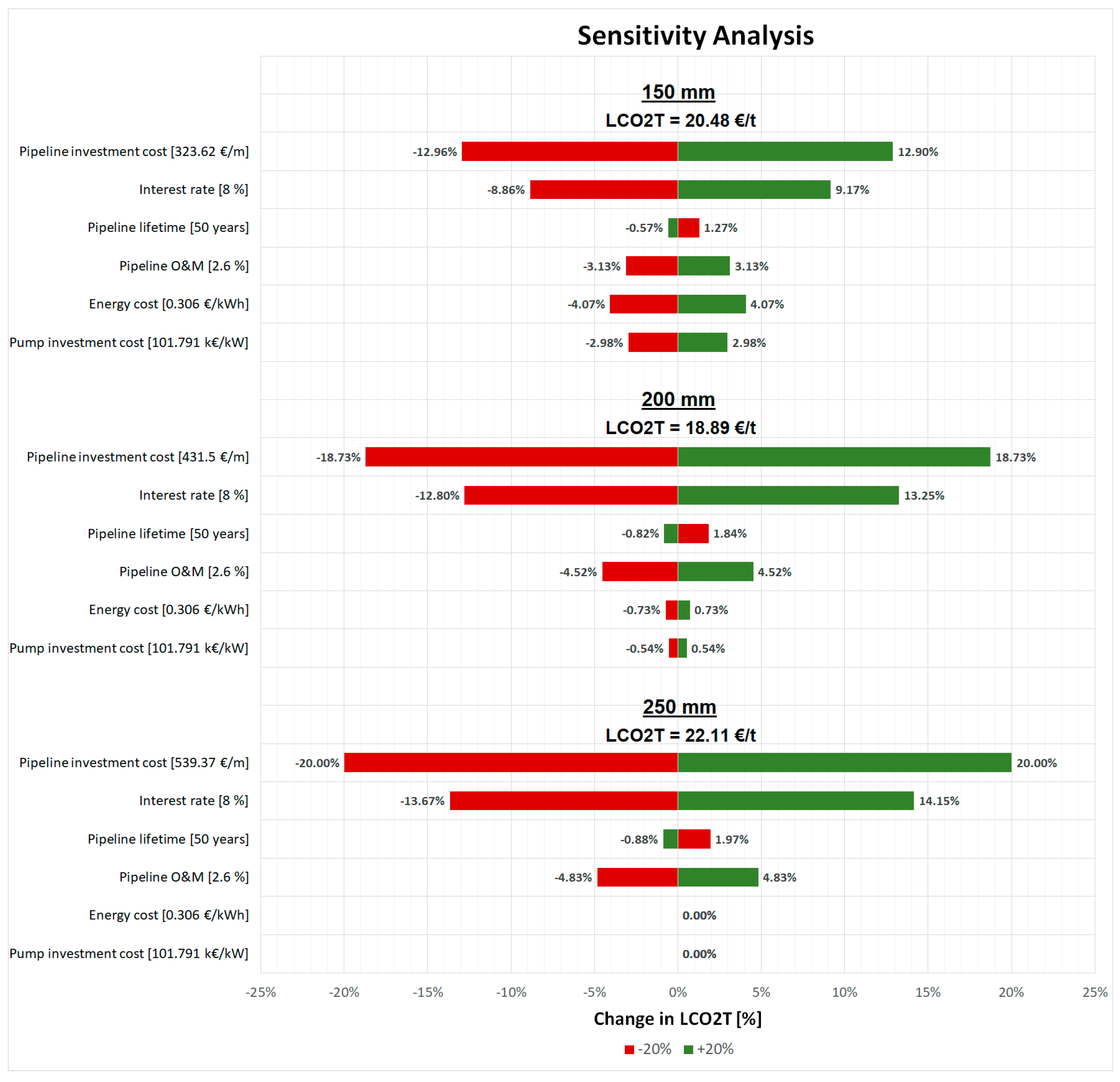
3.4. Sensitivity Analysis

Figure 14 depicts the results of a sensitivity analysis conducted to assess the influence of specific parameters on CO₂ transportation costs. The analysis varied factors such as pipeline and pump investment, interest rates, pipeline lifetime, pipeline O&M factor, and energy costs by ±20% to evaluate their impact on the total LCO2T. This sensitivity analysis was conducted for a case involving the transportation of 2000 t/day of CO₂ over a distance of 250 km, considering three different pipeline diameters: 150 mm, 200 mm, and 250 mm.

The sensitivity analysis highlights that pipeline investment exerts the most significant influence on the total LCO2T. In scenarios where booster stations are absent, pipeline investment becomes the primary contributor to the total LCO2T, particularly notable for the 250 mm diameter pipeline, where O&M costs are also a factor in the investment. Additionally, the interest rate significantly impacts the total LCO2T. Thus, the size and investment of the project play pivotal roles in determining the overall LCO2T. Factors such as pipeline lifetime and O&M have comparatively lesser impacts. Energy costs and pump investment are directly dependent on the number of booster stations required.

4. Conclusions

In this comprehensive study, a thorough examination of CO₂ transportation via pipelines has been undertaken, covering diverse aspects including pipeline diameters, costs, pressure drop considerations, and sensitivity analysis. By delving into both technical and economic aspects, this research offers a deeper understanding of the transport infrastructure associated with CO₂. Some key findings from the research are as follows:

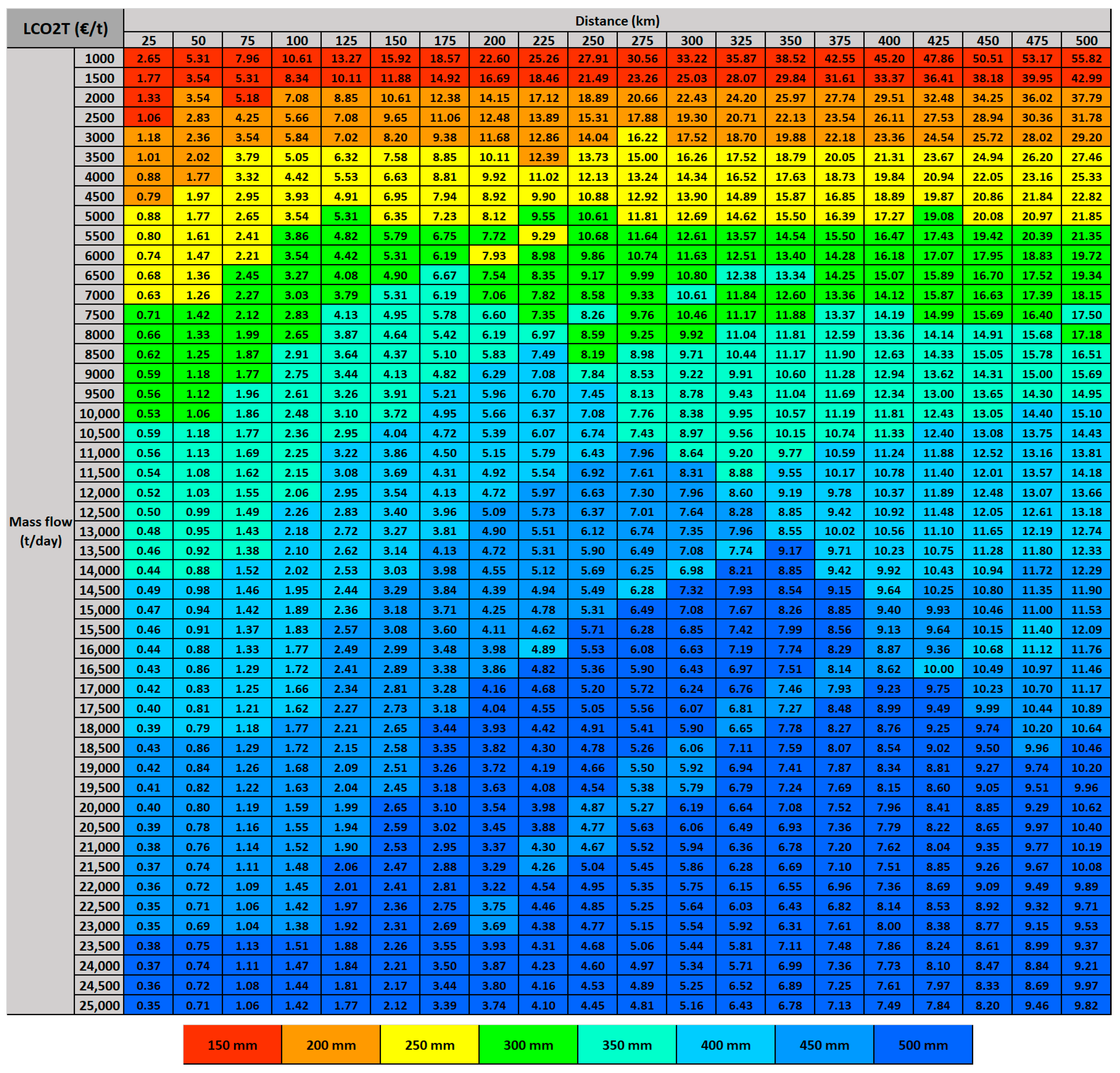
• Costs: The estimated levelized transport costs span a wide range, from 0.25 €/t to 55.82 €/t, depending on the transported mass, which varies from 1000 t/day to 25,000 t/day, and transport distances ranging from 25 km to 500 km. When factoring in initial compression costs, the LCO2T extends from 33.21 €/t to as high as 92.82 €/t for the same parameters. The calculated costs are based on various assumptions and serve as fundamental reference points for infrastructure planning.
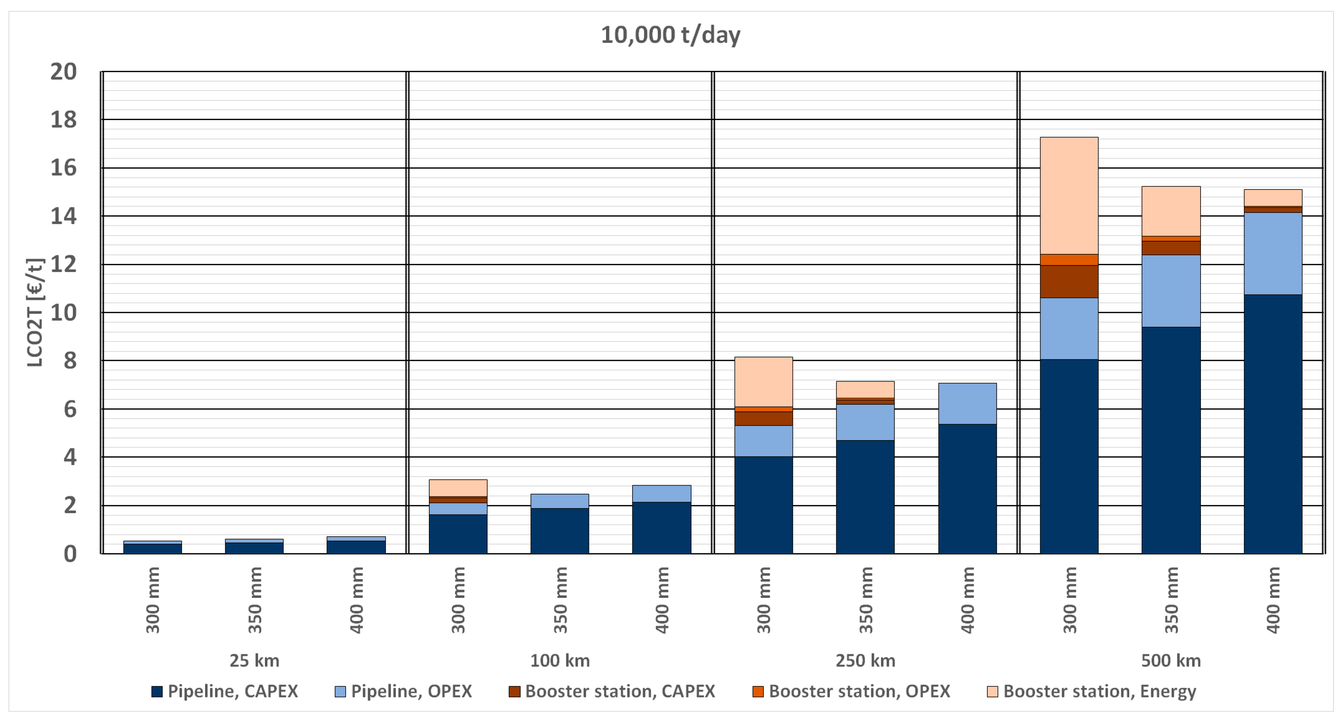
• Pipeline diameter: An analysis was conducted on eight different pipeline diameters, spanning from 150 mm to 500 mm. The resulting LCO2T calculations play a pivotal role in identifying the optimal pipeline diameter tailored to specific mass flow requirements and transport distances.
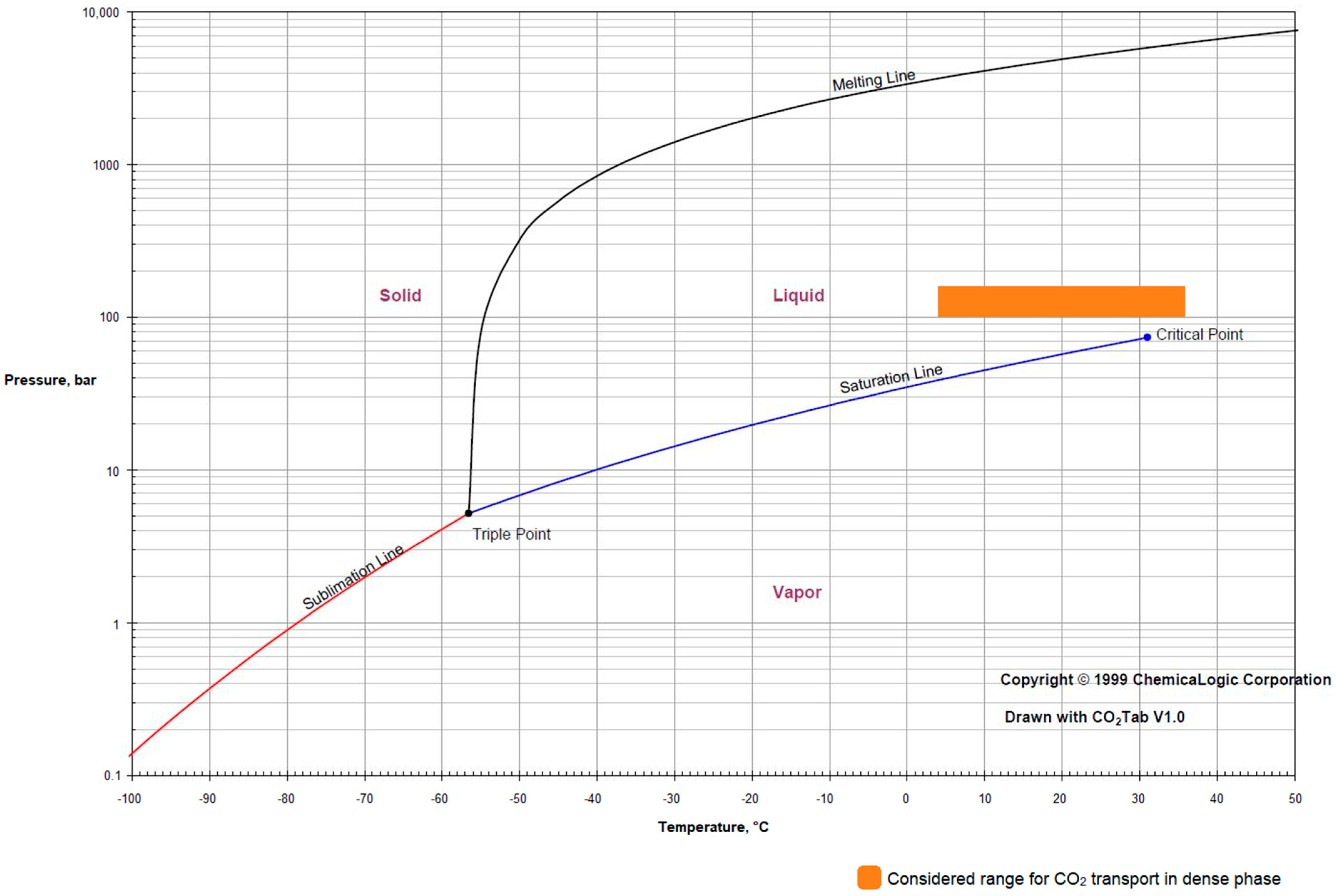
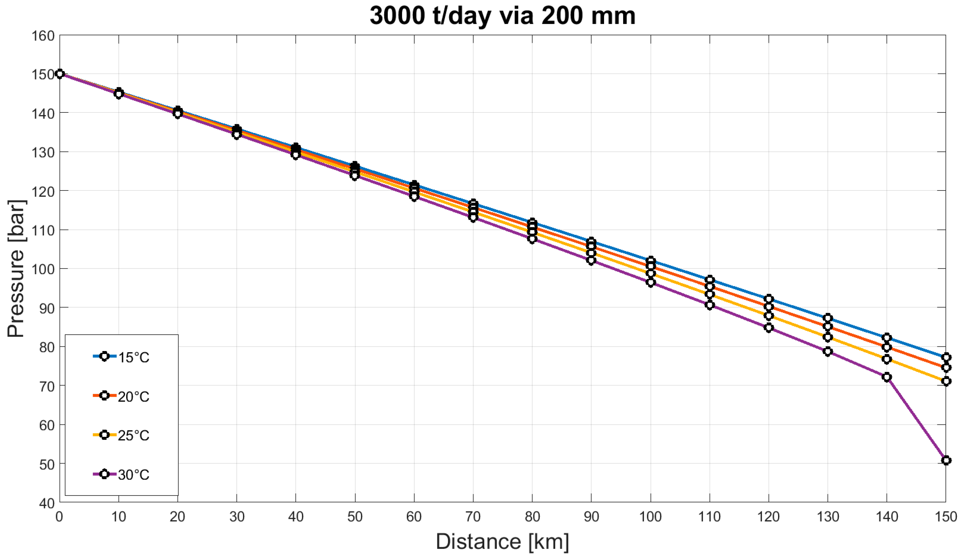
• Flow temperature: This research emphasizes the impact of CO₂ flow temperature within the pipeline. Elevated temperatures cause higher pressure loss, emphasizing the influence of environmental conditions on pipeline performance.
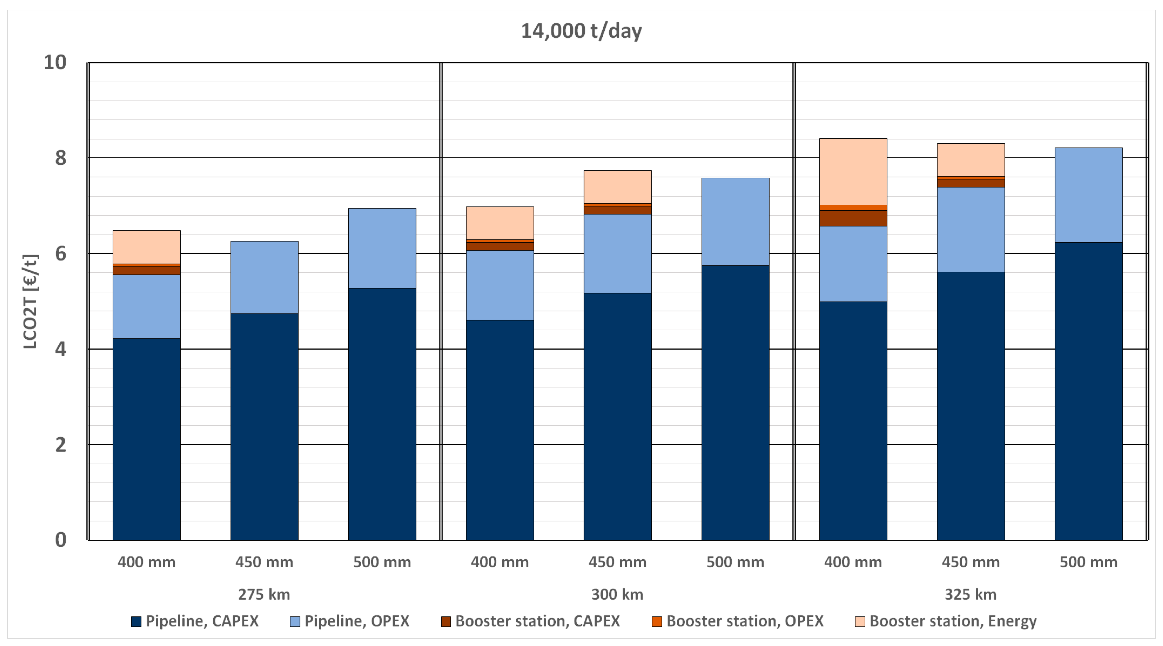
• Booster stations: Determining the exact distance at which a booster pump should be placed is one of the key highlights of this study. It is clear from the results that the number of booster stations plays a key role in determining the optimal diameter size, as it significantly impacts the total LCO2T.

In conclusion, the optimal pipeline diameter for transporting CO₂ depends on multiple factors including transport mass, distance, flow temperature, pressure loss along the pipeline, and the number of booster stations. Special considerations should also be given to pipeline investment, operational costs, energy costs, and interest rates to select the optimal transportation method. This comprehensive approach ensures efficient and cost-effective CO₂ transportation infrastructure planning.

Future research should expand on current findings by incorporating other transport modes such as trailers, trains, and ships. A deeper investigation of storage options, including offshore storage and the associated costs, should be conducted. Integrating factors such as carbon footprint and life cycle assessment into the analysis would provide a better understanding of the environmental impact of the transport infrastructure. Additionally, as decarbonization goals drive the shift from natural gas to clean fuels such as hydrogen, a study exploring the cost savings of planning both hydrogen and CO₂ pipelines together could be beneficial. Addressing these areas can provide a more comprehensive understanding of optimal strategies for cost-effective, efficient, and sustainable transport infrastructure.

References

1. BMWK. Kriterien zur Festlegung des Wasserstoff-Kernnetz Szenarios. Available online: https://www.bmwk.de/Redaktion/DE/Downloads/E/240226-eckpunkte-cms.pdf?__blob=publicationFile&v=8 (accessed on 17 May 2024).
2. Dalheimer. 20240226-Referentenentwurf-cms. Available online: https://www.bmwk.de/Redaktion/DE/Downloads/Gesetz/20240226-referentenentwurf-cms.pdf?__blob=publicationFile&v=10 (accessed on 17 May 2024).
3. Rüger, J.; Busse, A., Dr.; Röhrkasten, S., Dr. Eckpunkte Langzeitstrategie Negativemissionen. Available online: https://www.bmwk.de/Redaktion/DE/Downloads/E/240226-eckpunkte-negativemissionen.pdf?__blob=publicationFile&v=8 (accessed on 17 May 2024).
4. Wirtschaft und Klimaschutz, BMWK—Bundesministerium für. Bundesminister Habeck Will den Einsatz von CCS Ermöglichen: “Ohne CCS Können wir Unmöglich die Klimaziele Erreichen”. Available online: https://www.bmwk.de/Redaktion/DE/Pressemitteilungen/2024/02/20240226-habeck-will-den-einsatz-von-ccs-ermoeglichen.html (accessed on 17 May 2024).
5. IEA. Putting CO2 to Use. Available online: https://iea.blob.core.windows.net/assets/50652405-26db-4c41-82dc-c23657893059/Putting_CO2_to_Use.pdf (accessed on 17 May 2024).
6. Global Status of CCS 2021. Available online: https://ukccsrc.ac.uk/wp-content/uploads/2024/04/guloren-turan-global-status-of-ccs-2023.pdf (accessed on 17 May 2024).
7. Simonsen, K.R.; Hansen, D.S.; Pedersen, S. Challenges in CO2 transportation: Trends and perspectives. Renew. Sustain. Energy Rev. 2024, 191, 114149. [Google Scholar] [CrossRef]
8. Liu, E.; Lu, X.; Wang, D. A Systematic Review of Carbon Capture, Utilization and Storage: Status, Progress and Challenges. Energies 2023, 16, 2865. [Google Scholar] [CrossRef]
9. Lu, H.; Ma, X.; Huang, K.; Fu, L.; Azimi, M. Carbon dioxide transport via pipelines: A systematic review. J. Clean. Prod. 2020, 266, 121994. [Google Scholar] [CrossRef]
10. Wang, H.; Chen, J.; Li, Q. A Review of Pipeline Transportation Technology of Carbon Dioxide. IOP Conf. Ser. Earth Environ. Sci. 2019, 310, 32033. [Google Scholar] [CrossRef]
11. Onyebuchi, V.E.; Kolios, A.; Hanak, D.P.; Biliyok, C.; Manovic, V. A systematic review of key challenges of CO2 transport via pipelines. Renew. Sustain. Energy Rev. 2018, 81, 2563–2583. [Google Scholar] [CrossRef]
12. Peletiri, S.; Rahmanian, N.; Mujtaba, I. CO2 Pipeline Design: A Review. Energies 2018, 11, 2184. [Google Scholar] [CrossRef]
13. Hoa, L.Q.; Baessler, R.; Bettge, D. On the Corrosion Mechanism of CO2 Transport Pipeline Steel Caused by Condensate: Synergistic Effects of NO2 and SO2. Materials 2019, 12, 364. [Google Scholar] [CrossRef] [PubMed]
14. Porter, R.T.; Fairweather, M.; Pourkashanian, M.; Woolley, R.M. The range and level of impurities in CO2 streams from different carbon capture sources. Int. J. Greenh. Gas Control 2015, 36, 161–174. [Google Scholar] [CrossRef]
15. Zhao, Q.; Li, Y.-X. The influence of impurities on the transportation safety of an anthropogenic CO2 pipeline. Process Saf. Environ. Prot. 2014, 92, 80–92. [Google Scholar] [CrossRef]
16. Knoope, M.; Guijt, W.; Ramírez, A.; Faaij, A. Improved cost models for optimizing CO2 pipeline configuration for point-to-point pipelines and simple networks. Int. J. Greenh. Gas Control 2014, 22, 25–46. [Google Scholar] [CrossRef]
17. Grant, T.; Morgan, D.; Gerdes, K. Quality Guidelines for Energy System Studies: Carbon Dioxide Transport and Storage Costs in NETL Studies; DOE/NETL-2013/1614; National Energy Technology Laboratory (NETL): Pittsburgh, PA, USA; Morgantown, WV, USA; Albany, OR, USA, 2017. Available online: https://www.osti.gov/biblio/1557135 (accessed on 17 May 2024).
18. Mohammadi, M.; Hourfar, F.; Elkamel, A.; Leonenko, Y. Economic Optimization Design of CO2 Pipeline Transportation with Booster Stations. Ind. Eng. Chem. Res. 2019, 58, 16730–16742. [Google Scholar] [CrossRef]
19. Rubin, E.S.; Davison, J.E.; Herzog, H.J. The cost of CO2 capture and storage. Int. J. Greenh. Gas Control 2015, 40, 378–400. [Google Scholar] [CrossRef]
20. Grant, T.; Poe, A.; Valenstein, J.; Guinan, A.; Shih, C.; Lin, S. Quality Guidelines for Energy System Studies: Carbon Dioxide Transport and Storage Costs in NETL Studies; National Energy Technology Laboratory (NETL): Pittsburgh, PA, USA; Morgantown, WV, USA, 2019. Available online: https://www.osti.gov/biblio/1567735 (accessed on 17 May 2024).
21. Mallon, W.; Buit, L.; van Wingerden, J.; Lemmens, H.; Eldrup, N.H. Costs of CO2 Transportation Infrastructures. Energy Procedia 2013, 37, 2969–2980. [Google Scholar] [CrossRef]
22. Global CCS Institute. The Costs of CO2 Transport: Post-Demonstration CCS in the EU—Global CCS Institute. Available online: https://www.globalccsinstitute.com/resources/publications-reports-research/the-costs-of-co2-transport-post-demonstration-ccs-in-the-eu/ (accessed on 26 March 2024).
23. Correia, S.d.S.J.; Morbee, J.; Tzimas, E. Technical and Economic Characteristics of a CO2 Transmission Pipeline Infrastructure; Publications Office of the European Union: Luxembourg, 2011; ISNN 1018-5593. [Google Scholar] [CrossRef]
24. Knoope, M.; Ramírez, A.; Faaij, A. A state-of-the-art review of techno-economic models predicting the costs of CO2 pipeline transport. Int. J. Greenh. Gas Control 2013, 16, 241–270. [Google Scholar] [CrossRef]
25. Hydrogen Delivery Scenario Analysis Model. Available online: https://hdsam.es.anl.gov/index.php?content=hdsam (accessed on 26 March 2024).
26. Solomon, M.D.; Heineken, W.; Scheffler, M.; Birth-Reichert, T. Cost Optimization of Compressed Hydrogen Gas Transport via Trucks and Pipelines. Energy Technol. 2024, 12, 2300785. [Google Scholar] [CrossRef]
27. Witkowski, A.; Majkut, M.; Rulik, S. Analysis of pipeline transportation systems for carbon dioxide sequestration. Arch. Thermodyn. 2014, 35, 117–140. [Google Scholar] [CrossRef]
28. Jackson, S. Development of a Model for the Estimation of the Energy Consumption Associated with the Transportation of CO2 in Pipelines. Energies 2020, 13, 2427. [Google Scholar] [CrossRef]
29. McCollum, D.L.; Ogden, J.M. Techno-Economic Models for Carbon Dioxide Compression, Transport, and Storage & Correlations for Estimating Carbon Dioxide Density and Viscosity; Institute of Transportation Studies: Davis, CA, USA, 2006. [Google Scholar]
30. Deng, H.; Roussanaly, S.; Skaugen, G. Techno-economic analyses of CO2 liquefaction: Impact of product pressure and impurities. Int. J. Refrig. 2019, 103, 301–315. [Google Scholar] [CrossRef]
31. Bell, I.H.; Wronski, J.; Quoilin, S.; Lemort, V. Pure and Pseudo-pure Fluid Thermophysical Property Evaluation and the Open-Source Thermophysical Property Library CoolProp. Ind. Eng. Chem. Res. 2014, 53, 2498–2508. [Google Scholar] [CrossRef] [PubMed]
32. CO2Tab Downloads. Available online: http://www.chemicalogic.com/Pages/CO2TabDownloads.html (accessed on 6 May 2024).
33. Kreutz, T.; Williams, R.; Consonni, S.; Chiesa, P. Co-production of hydrogen, electricity and CO from coal with commercially ready technology. Part B: Economic analysis. Int. J. Hydrog. Energy 2005, 30, 769–784. [Google Scholar] [CrossRef]
34. €1 in 2010 → 2024|Germany Inflation Calculator. Available online: https://www.officialdata.org/germany/inflation/2010?amount=1 (accessed on 6 May 2024).
35. Pipeline Transmission of CO2 and Energy Transmission Study–Report; IEA Greenhouse Gas R&D Programme: Cheltenham, UK, 2002.
36. The Danish Energy Agency. Technology Data for Carbon Capture, Transport and Storage. Available online: https://ens.dk/en/our-services/projections-and-models/technology-data/technology-data-carbon-capture-transport-and (accessed on 26 March 2024).
37. Wildenborg, T.; Gale, J.; Hendriks, C.; Holloway, S.; Brandsma, R.; Kreft, E.; Lokhorst, A. Cost curves for CO2 storage: European sector. In Greenhouse Gas Control Technologies 7; Elsevier Science Ltd.: Amsterdam, The Netherlands, 2005; pp. 603–610. [Google Scholar] [CrossRef]
38. Heddle, G.; Herzog, H.; Klett, M. The Economics of CO2 Storage; Massachusetts Institute of Technology, Laboratory for Energy and the Environment: Cambridge, MA, USA, 2003. [Google Scholar]
39. Piessens, K.; Laenen, B.; Nijs, W.; Mathieu, P.; Baele, J.M.; Hendriks, C.; Bertrand, E.; Bierkens, J.; Brandsma, R.; Broothaers, M.; et al. Policy Support System for Carbon Capture and Storage; Relatório final para a Science for a Sustainable Development (SSD), 2008; Available online: https://www.belspo.be/belspo/SSD/science/Reports/PSS-CCS_FinRep_2008.DEF.pdf (accessed on 17 May 2024).
40. Turgut, O.E.; Asker, M.; Çoban, M.T. A review of non iterative friction factor correlations for the calculation of pressure drop in pipes. Bitlis Eren Univ. J. Sci. Technol. 2014, 4, 1–8. [Google Scholar] [CrossRef]
41. Solomon, M.D.; Heineken, W.; Scheffler, M.; Birth-Reichert, T. Pressure Drop In Pipelines Transporting Compressed Hydrogen Gas. Energy Technol. 2023, 12, 2300785. [Google Scholar] [CrossRef]
Figure 1. CO2 processing block diagram.
Energies 17 02911 g001
Figure 2. CO2 phase diagram [32].
Energies 17 02911 g002
Figure 3. Pressure drop at different temperatures.
Energies 17 02911 g003
Figure 4. Pressure drop in a pipeline with a 200 mm diameter.
Energies 17 02911 g004
Figure 5. Pressure drop in a pipeline with a 300 mm diameter.
Energies 17 02911 g005
Figure 6. Detailed cost breakdown of LCO2T for transporting 10,000 t/day over different distances.
Energies 17 02911 g006
Figure 7. Least levelized transport cost of CO2 for different mass flow and distances.
Energies 17 02911 g007
Figure 8. Least levelized transport cost of CO2 inclusive of initial compression.
Energies 17 02911 g008
Figure 9. Detailed cost breakdown for transporting 14,000 t/day.
Energies 17 02911 g009
Figure 10. Pressure drop when transporting 14,000 t/day at different diameters.
Energies 17 02911 g010
Figure 11. Detailed cost breakdown for a distance of 300 km at different mass flow rates.
Energies 17 02911 g011
Figure 12. Detailed cost breakdown for a distance of 300 km at different mass flow rates.
Energies 17 02911 g012
Figure 13. No. of booster stations required for each case.
Energies 17 02911 g013
Figure 14. Sensitivity analysis.
Energies 17 02911 g014