Abstract
Sheet Molding Compound (SMC) materials are extensively utilized as high-voltage insulation materials in electrical equipment. SMC materials are prone to aging after long-term operation. Conducting non-destructive testing to assess their electrical and physicochemical properties is crucial for the safe operation of electrical equipment. This study identifies the optimal equipment parameters for testing SMC materials using Laser-Induced Breakdown Spectroscopy (LIBS) technology through experimental investigation and also explores the ablation characteristics of SMC under various laser parameters. The results indicate a significant positive correlation between the ablation depth and laser pulse number, while there is no correlation with single laser pulse energy. However, the ablation area demonstrates a strong positive correlation with both single laser pulse energy and laser pulse number. Additionally, LIBS spectral analysis provides elemental results comparable to Energy Dispersive Spectroscopy (EDS), facilitating the examination of variations in Na, Ti, Fe, Mg, Ca, and C elemental contents with depth. Moreover, an enhanced iterative Boltzmann plot method is suggested for calculating the plasma temperature using 21 Fe I spectral lines and the electron density using the Fe II 422.608 nm line. The variations of these plasma parameters with laser pulse number are documented, and the results show consistent trends, confirming that the laser-induced SMC plasma adheres to local thermodynamic equilibrium.
1. Introduction
Laser-Induced Breakdown Spectroscopy (LIBS) technology has witnessed rapid development within a few years. It utilizes a high-energy laser pulse to ablate the sample surface and generate a transient plasma. This plasma emits characteristic spectra during cooling, which could be used for sample analysis [1,2]. LIBS has garnered great attention from researchers due to its nearly non-destructive testing, low detection limits, high sensitivity, real-time analysis ability, and wide applicability, and has shown promising application prospects. Furthermore, the high brightness, high coherence, and low divergence exhibited by lasers make it easy for the laser beam to be focused at very high power over very long distances onto extremely small points [3], enabling long-distance detection to be possible. Since its introduction in the late 1980s, LIBS technology has been successfully applied in industrial diagnostics [4,5], agricultural testing [6,7], environmental protection [8,9,10], biomedical research [11,12,13], cultural heritage preservation [14,15], and various other fields.
In the field of electrical engineering, numerous scholars have applied LIBS technology to the analysis of electrical equipment. Wang Xilin’s team has achieved significant results in using LIBS to detect electrical composite insulators. They successfully developed a hardness prediction model using LIBS to assess the aging condition of composite materials [16]. Additionally, they applied LIBS to study surface contamination issues on insulators. By integrating Principal Component Analysis (PCA), k-means clustering, and Partial Least Squares Regression (PLSR), they accomplished quantitative detection of metal contamination on high-voltage transmission line insulators [17]. This method also distinguished between algal contamination, non-algal contamination, and uncontaminated conditions [18]. Sanjana and colleagues [19] utilized LIBS and machine learning techniques to classify contaminated silicone rubber insulators. Through LIBS analysis and employing various machine learning algorithms for classification, light gradient boosting technology demonstrated the highest classification accuracy of 97.43%. Babu and others [20] used LIBS technology to analyze the pollution performance of epoxy-alumina nanocomposite materials. An ANN trained with the Polak–Ribiere updated conjugate gradient backpropagation algorithm is used in classification, achieving an accuracy of up to 100%. Gondal and colleagues [21] utilized LIBS technology to detect ion species in cables, revealing the presence of abundant Na and Cl ions. Analysis of various polymer samples indicated a correlation between cable quality and the content of ion species in the raw materials. Neettiyath and colleagues analyzed pollutants in the insulation material of high-voltage transformer oil-immersed paper with Vacuum Ultraviolet LIBS technology [22]. They further utilized LIBS and Thermogravimetric Analysis (TGA) to study the relationship between the lifespan of oil-impregnated paperboard and temperature variations, realizing the prediction of the lifespan of thermally aged oil-impregnated paperboard [23]. Amlanathan and his team performed LIBS analysis on heat-aged ester-impregnated paperboard, verifying the degradation of the paperboard material. By combining PCA and neural network analysis, they accurately distinguished between aged and unaged paperboard samples [24]. Yuan introduced the enhancing effect of spark discharge on the detection of iron particles in transformer oil using LIBS. By optimizing circuit parameters to amplify the Fe spectrum, they enhanced the quantitative limit of LIBS from 0.048 μg g−1 to 0.016 μg g−1, markedly improving the technology’s ability to detect particles in oil [25].
Sheet Molding Compound (SMC) is a type of glass fiber-reinforced unsaturated polyester thermosetting plastic. It consists of a thermosetting resin matrix and glass fibers. The application of SMC material in the electrical field is primarily due to its insulation properties, corrosion resistance, thermal insulation performance [26], and mechanical strength, making it an ideal choice for manufacturing electrical equipment and components. It is mainly used in the production of electrical equipment enclosures, high-voltage insulating boards, electrical connectors, and cable brackets.
SMC materials are commonly used as insulation materials in electrical equipment; however, their various qualities on the market pose numerous risks. Additionally, these materials face issues like aging, declining insulation performance, and weakening mechanical properties, which are detrimental to the safe and stable operation of electrical equipment. Currently, although many researchers have applied LIBS to the testing of electrical materials, studies specifically on SMC materials are limited. Therefore, it is essential to conduct research on the testing of SMC materials. We aim to use LIBS technology to perform quality tests on SMC materials to ensure the safety of electrical equipment and to characterize the performance of SMC materials, assessing their service state. This article focuses on using LIBS technology to study SMC materials, emphasizing parameter optimization for LIBS testing, material ablation, spectral and plasma parameter analysis of LIBS, and systematic analysis of SMC materials using Scanning Electron Microscope (SEM), Energy Dispersive Spectroscopy (EDS), and Confocal Laser Scanning Microscope (CLSM). This research aims to support further characterization studies of SMC materials in electrical equipment using LIBS, demonstrating that LIBS is theoretically feasible and minimally damaging to the materials.
2. Materials and Methods
2.1. Materials
The materials utilized in this study include white SMC high-voltage insulating board (Zhejiang Haode Sheng Insulation Materials Company, Hangzhou, China). This composite material exhibits excellent electrical insulation properties and is resistant to high temperatures and voltages. It is primarily made of unsaturated resin and glass fiber. The dimensions of the sample are 80 mm × 15 mm × 4 mm.
2.2. Equipment
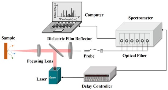
The schematic diagram of the LIBS system, depicted in Figure 1, primarily comprises a laser (Lei Bao Optoelectronics Company, Beijing, China), a delay controller (Stanford Research Systems, CA, USA), a spectrometer (Beijing Avantes Co., Ltd., Beijing, China), an optical path, and a fiber probe (Beijing Avantes Co., Ltd., Beijing, China). The medium mirror within the optical path is designed to reflect the incident laser at specific wavelengths with exceptionally high reflectivity while simultaneously allowing signals in the visible light spectrum to pass through unimpeded. The laser generates pulsed beams, which are then reflected by the reflector onto a long-focal-length focusing lens. This lens focuses the laser onto the sample’s surface, inducing ablation and plasma formation. As the plasma cools, it emits characteristic spectra. Some of these spectral signals are captured by the long focal length focusing lens and subsequently reflected by the medium mirror onto a short focal length lens. These signals are then focused, collected by the fiber probe, and transmitted to the computer for analysis via the spectrometer.
The laser utilized in the experiment is a nanosecond Nd: YAG laser (Nimma-900 model) from Lei Bao Optoelectronics Company (Beijing, China). It is capable of emitting four distinct wavelengths: 1064 nm, 532 nm, 355 nm, and 266 nm, which can be converted through switching. For this experiment, the 1064 nm wavelength was chosen due to its excellent energy stability, minimal attenuation in air, a maximum single pulse energy of 900 mJ, a pulse width of ≤9 ns, an operating frequency ranging from 1 Hz to 10 Hz, and its functionality in an external trigger mode.
The spectrometer employed is the Avantes (Beijing, China) AVS-RACKMOUNT -USB2, featuring a wavelength range of 200 nm to 640 nm and a resolution between 0.09 nm and 0.13 nm. To collect the spectral signal at a 45° angle, a convex lens with a 6 cm diameter was selected. The distance from the convex lens to the ablation point on the sample was adjusted to maximize the collection of light signals emitted by the plasma. The fiber probe was positioned at the focal point of the convex lens. The spectrometer converts and stores the collected signals using the Avasoft 8.16 software.
The employed signal delay generator is the eight-channel digital delay generator DG645, offering a delay resolution of 5 ps across all channels. The jitter among channels is under 25 ps, with delay control accuracy at 1 ns. This generator is instrumental in setting the laser and spectrometer delay, emitting the Q-switch trigger signal for the laser, and using the external trigger signal for the spectrometer to manage the timing sequence.
2.3. Data Processing
By normalizing the spectral data, we mitigate the effects of fluctuations in parameters such as pulse energy and measurement efficiency while also diminishing the matrix effect. The resulting normalized spectrum is depicted in Figure 2a. This study employs Discrete Wavelet Transformation (DWT) for baseline correction and noise reduction in the normalized spectrum. As illustrated in Figure 2b, the majority of the noise has been significantly removed, and the spectral lines across different channels have been accurately corrected. Following the preprocessing of the spectral data, peak finding becomes essential, as it significantly influences the precision of the analysis results. This study adopts the Continuous Wavelet Transform (CWT) method for peak finding, which is adept at identifying overlapping peaks with high accuracy.
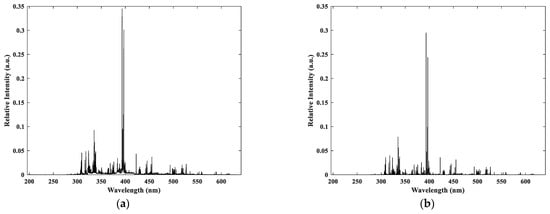
Figure 2.
Spectral data processing results: (a) Area normalization processing; (b) Baseline correction and denoising processing.
As shown in Figure 3, the peak-finding results are satisfactory, effectively identifying the majority of the spectral peaks. Some peaks with weak intensities are not labeled; however, since lower-intensity peaks are typically ignored during spectral analysis, this does not affect the accuracy of the analysis.
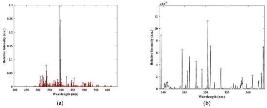
Figure 3.
Spectral automatic peak finding results: (a) Overall peak finding effect; (b) Local peak finding effect.
In this study, considering both the accuracy of element identification and computational time, the Atomic Spectra Database (ASD) from the National Institute of Standards and Technology (NIST) was referenced [27]. The center wavelengths corresponding to the tested spectral peaks were compared with the standard wavelengths in the database to determine the elemental attribution of the spectral lines. By referencing the information in the NIST database, six characteristic spectral lines with relatively high intensities were selected for research analysis, namely Na II 317.906 nm, Ti II 334.940 nm, Fe I 338.398 nm, Mg I 383.829 nm, Ca II 393.366 nm, and C I 396.140 nm.
3. Results and Discussion
3.1. Optimization of LIBS Technical Parameters
3.1.1. Delay Time
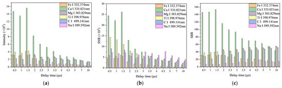
The laser-induced plasma generated during LIBS detection evolves rapidly. However, it is susceptible to interference from background spectra and noise, making it challenging to accurately detect trace elements with weak radiation. To obtain stable and accurate signals, selecting an appropriate delay time is necessary to ensure higher intensities of characteristic spectral lines, signal-to-noise ratio (SNR), and signal-to-background ratio (SBR). The delay time of the spectrometer was controlled using a signal generator with 12 different levels: 0.5, 1, 1.5, 2, 2.5, 3, 3.5, 4, 4.5, 5, 7, and 10 μs. The laser energy was set at a fixed single-pulse energy of 45 mJ. Under these conditions, the LIBS spectral lines were clear.
Figure 4a illustrates that the intensity of the characteristic spectral lines—Fe I 338.398 nm, Ca II 393.366 nm, Mg I 383.829 nm, Ti II 334.940 nm, C I 396.140 nm, and Na II 317.906 nm—generally decreases as the delay time increases, with a minor change observed after 4 μs. With the prolongation of delay time, the signal-to-noise ratio (SNR) of these spectral lines tends to decline. Notably, at 1.5 μs, the SNR for Fe I 338.398 nm, Ca II 393.366 nm, and C I 396.140 nm spectral lines exhibits an increase (as depicted in Figure 4b). Furthermore, with an extension in delay time, except for Fe I 338.398 nm and Ca II 393.366 nm, the signal-to-background ratio (SBR) of the remaining characteristic spectral lines generally exhibits an upward trend, stabilizing after 3 μs (shown in Figure 4c). Considering all factors, a delay time of 1.5 μs is selected for its relatively high intensity of the characteristic spectral lines, alongside superior SNR and SBR values.
3.1.2. Single Laser Pulse Energy
When the laser energy is insufficient, it fails to reach the breakdown threshold of the sample, therefore preventing plasma generation. Conversely, excessively high laser energy can induce shielding effects from the plasma, leading to significant damage to the sample’s surface. Thus, selecting optimal laser energy is crucial. The laser’s single pulse energy was adjusted to seven distinct levels: 35, 45, 55, 65, 75, 85, and 95 mJ. As depicted in Figure 5a, aside from the unclear spectral intensity trend of Na II at 317.906 nm, the intensities of the other five characteristic spectral lines exhibit an upward trend as the laser energy increases. Specifically, Ca II at 393.366 nm demonstrates a more rapid increase, whereas the remaining lines show a more gradual rise. In Figure 5b, the SNR of Fe I at 338.398 nm, Ti II at 334.940 nm, and Ca II at 393.366 nm significantly increases with higher laser energy, while the SNR of the other lines remains relatively unchanged. Figure 5c reveals a modest rise in the SBR of Ca II 393.366 nm with increased laser energy, with the SBR of other lines displaying negligible variations. This study selected a single pulse laser energy of 45 mJ, which provides a sufficiently strong spectrum for analysis while minimizing damage to the sample.
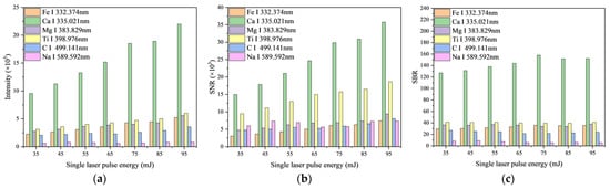
Figure 5.
Variation in spectral parameters with single laser pulse energy: (a) Change of characteristic spectral line intensity with single laser pulse energy; (b) Change of characteristic spectral line SNR with single laser pulse energy; (c) Change of characteristic spectral line SBR with single laser pulse energy.
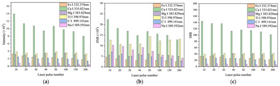
3.1.3. Laser Pulse Number
The number of laser pulses also impacts the precision of detection. Insufficient pulses may not yield adequate data, whereas excessive pulses could harm the sample. Consequently, the number of laser pulses was adjusted to eight distinct levels: 10, 20, 30, 40, 50, 100, 150, and 200 pulses.
The findings in Figure 6a reveal that the overall intensity of the spectral lines diminishes as the number of laser pulses increases, with a notable uptick in intensity at 50 pulses. Similarly, in Figure 6b, the signal-to-noise ratio (SNR) exhibits a comparable pattern to the line intensity, which initially declined but then experienced a marked improvement at either 40 or 50 pulses. As depicted in Figure 6c, the signal-to-background ratio (SBR) of Ca II 393.366 nm, Fe I 338.398 nm, C I 396.140 nm, and Na II 317.906 nm declines as the number of laser pulses increases, whereas the remaining characteristic spectral lines generally show an upward trend. Taking intensity, SNR, SBR, and the risk of sample damage into account, a laser pulse number of 20 was selected.
3.2. Laser Ablation Characteristics of SMC
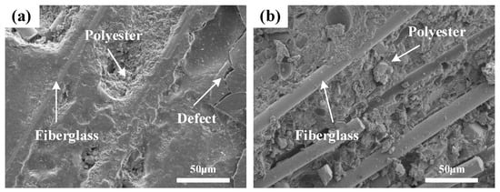
Figure 7 displays the microstructure observed by the SEM, revealing defects on the sample surface alongside distinct rod-shaped glass fibers and resin particles (Figure 7a). The internal glass fibers and resin particles are uniformly mixed, suggesting that the breakage of glass fibers could be damage inflicted on the sample during its preparation (Figure 7b).
3.2.1. Effect of Laser Pulse Number
Conduct LIBS testing on the sample using a constant single laser pulse energy of 45 mJ, a delay time of 1.5 μs, and varying laser pulse numbers of 10, 50, 100, 150, 200, 250, and 300. Perform SEM testing on the ablation sites, with the microstructure displayed in Figure 8.
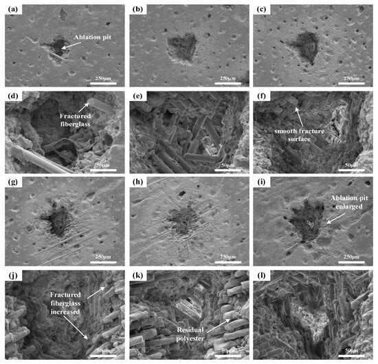
Figure 8.
Microscopic morphology of samples under different laser pulse number: (a–c,g–i) show the overall morphology of ablation pits after 10, 50, 100, 150, 200, and 300 laser pulses, respectively; (d–f,j–l) depict the corresponding internal morphology of the ablation pits.
As the number of laser pulses increases, the pit formed on the material’s surface enlarges. With 10 laser pulses, the ablation pit contains a few glass fiber fractures, specifically the breaking of Si-O bonds, totaling around 5 fractures. As the number of laser pulses rises, the fractures increase to approximately 16 at 50 pulses, about 26 at 100 pulses, and close to 80 fractures at 200 pulses. The appearance of the glass fiber fractures also significantly changes. Initially, at 10 pulses, the fracture surface is rough, but it smoothens at 100 pulses due to the repeated laser impacts on the glass fiber fractures, where the accumulated energy causes the fracture surfaces to melt.
3.2.2. Effect of Single Laser Pulse Energy
With a constant laser pulse count of 100, the energy of each pulse is adjusted to the following values: 35, 45, 55, 65, 75, 85, and 95 mJ. SEM analysis is performed on the ablation sites of the sample, as depicted in Figure 9.
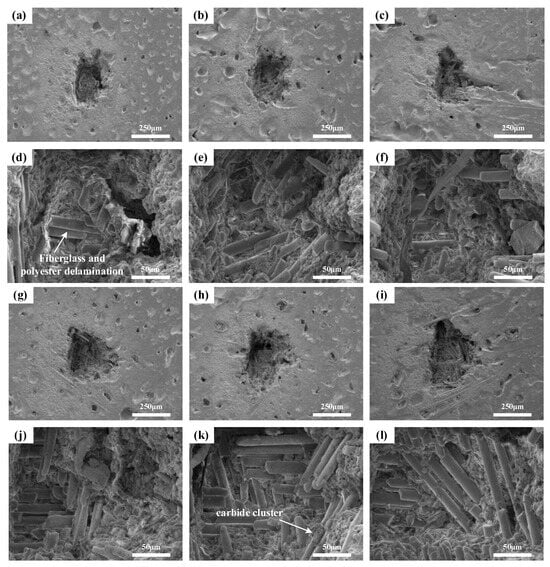
Figure 9.
Microscopic morphology of samples under different single laser pulse energy: (a–c,g–i) represent the overall morphology of ablation pits at single laser pulse energies of 45 mJ, 55 mJ, 65 mJ, 75 mJ, 85 mJ, and 95 mJ, respectively; (d–f,j–l) show the corresponding internal morphology of the ablation pits.
The morphology of the ablation pit surface and interior, similar to the experiment with varying laser pulse numbers, displays glass fiber fractures and predominantly smooth fracture surfaces due to 100 laser pulses. However, a notable increase in the ablation pit size is only observed when the single laser pulse energy reaches over 75 mJ. The laser energy applied to the sample induces thermal decomposition of the resin, leading to the detachment of glass fibers from the resin, the creation of gaps between the fibers, and some residual resin remaining on top. With an increase in the single laser pulse energy, the resin decomposition becomes more thorough, resulting in a reduction in the amount of residual resin on the fibers and a rise in the number of detached fibers. As the energy continues to escalate, the resin undergoes pyrolysis, and the ablation products consolidate into several large agglomerates. Approximately 24 glass fibers fracture at an energy of 45 mJ, about 41 fibers at 55 mJ, around 49 fibers at 65 mJ, approximately 28 fibers at 75 mJ, roughly 46 fibers at 85 mJ, and about 75 fibers at 95 mJ.
3.2.3. Ablation Characteristics and Laser Parameters Relationship
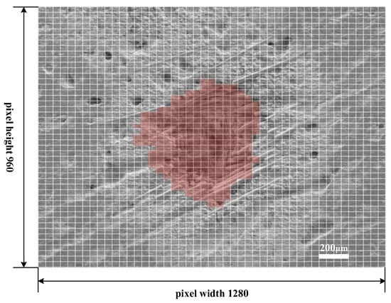
Based on SEM micrographs, this paper estimates the area of ablation pit surfaces using a grid method, as illustrated in Figure 10. The micrograph shows the morphology of an ablation pit following 250 laser pulses, captured at an image pixel resolution of 1280 × 960. A 47 × 47 grid is superimposed on the image, with each grid square measuring 50 μm in length and 37.5 μm in width, determined by the scale and dimensions of the image.
It has been observed that as the number of laser pulses increases, both the average ablation depth and the ablation surface area exhibit a linear growth trend (Table 1). Compared to 10 laser pulses, at 300 laser pulses, there is a significant increase in both the ablation depth and surface area, yet the ablation area remains relatively small, causing minimal damage to the sample. The rise in ablation depth and surface area also accounts for the increased number of fractured glass fibers.

With an increase in single-pulse laser energy, the average ablation depth shows relatively little fluctuation, averaging at 348.959 μm (Table 2). This suggests that the number of laser pulses has a more pronounced effect on ablation depth than single-pulse laser energy does. The variation in ablation pit surface area remains minimal when the energy is below 65 mJ but experiences a significant increase after reaching 75 mJ.
To better comprehend the correlation between laser parameters and both the average ablation depth and ablation area, respectively, this study performed linear fitting of these variables in relation to the number of laser pulses and the energy of a single laser pulse, as depicted in Figure 11 and Figure 12.
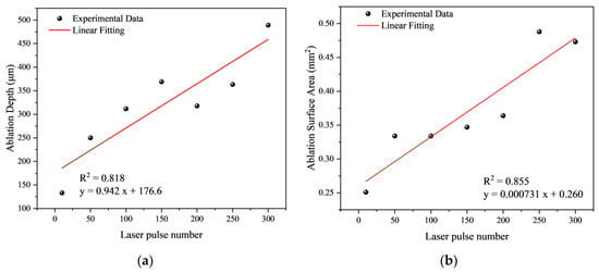
Figure 11.
Fitting the curve of ablation parameters with the laser pulse number: (a) Fitting curve of ablation depth with laser pulse number; (b) Fitting curve of ablation area with laser pulse number.
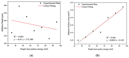
Figure 12.
Fitting curve of ablation parameters with single laser pulse energy: (a) Fitting curve of ablation depth with single laser pulse energy; (b) Fitting curve of ablation area with single laser pulse energy.
Utilizing the least squares fitting method, a linear fit was applied to the relationship between ablation depth and the number of laser pulses (Figure 11a). The correlation coefficient of the fitted curve is 0.904 (R2 = 0.818), indicating a good fit. Additionally, there is a strong positive correlation (R2 = 0.855) between the ablation area and the number of laser pulses (Figure 11b).
Similarly, fittings were conducted to explore the relationships between average ablation depth, ablation area, and single laser pulse energy. The fitting coefficient between average ablation depth and single laser pulse energy (R2 = 0.095) suggests a poor fit (Figure 12a), and it cannot be considered a negative correlation. Conversely, the fitting coefficient for the fitting curve between ablation area and single laser pulse energy is 0.940 (Figure 12b), indicating a strong positive correlation between the two.
3.3. LIBS Analysis of the SMC
3.3.1. Element Analysis
Using a single laser pulse energy of 45 mJ, 20 laser pulses, and a delay time of 1.5 μs, we performed LIBS testing on the sample. The spectrum, spanning the wavelength range of 250 to 550 nm, is depicted in Figure 13, with the spectral line intensity normalized.
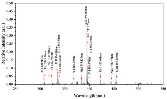
Analyzing the LIBS spectrum revealed that the SMC sample comprises elements such as Fe, Na, Ti, Mg, Ca, C, Al, and Si.
Table 3 displays the elemental content results obtained from EDS testing performed on the sample. While the quantitative results may not be precise, they still confirm the presence of C, O, Na, Mg, Al, Si, K, Ca, Ti, and Fe elements in the sample. Most elements were detected by LIBS, with the exceptions of O, S, Cl, K, and Pt. The significant presence of O atoms in the sample is theoretically expected, yet due to the weak spectral line intensity of O plasma, the O element was not detected. S, Cl, and K elements were not identified owing to their low concentrations. Pt was applied to the sample surface during EDS testing to enhance conductivity, meaning the sample itself does not contain Pt.
3.3.2. Elemental Content Varies with Depth
Under the conditions of a single laser pulse energy of 45 mJ and a delay time of 1.5 μs, LIBS testing was performed on the sample. The variation in element content, including Na, Ti, Fe, Mg, Ca, and C, with the number of laser pulses is depicted in Figure 14. The fluctuation in spectral line intensity indicates changes in element content.
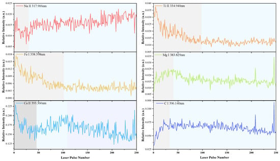
According to the findings in Section 3.2.3, a positive correlation exists between ablation depth and the number of laser pulses. Consequently, observing the relationship between element content and depth within the testing range can lead to the following conclusions:
- -
- The Na content remains relatively constant, with minimal variation as depth changes.
- -
- The content of Ti and Fe elements decreases with increasing depth;
- -
- The Mg and C content initially rises and then falls with depth;
- -
- The Ca element content shows a complex pattern, which decreases initially, then increases, and finally decreases again.
This study posits that the variation in these element contents is primarily due to the sample being a composite material made of glass fiber and unsaturated resin, which cannot be uniformly mixed at a microscopic level, leading to an uneven distribution of various elements.
3.3.3. Plasma Parameters
The laser-induced plasma state undergoes rapid evolution, and the plasma temperature and electron density that characterize its state also change rapidly. The evolution of the plasma state has a significant impact on the repeatability and accuracy of the LIBS signals. By analyzing parameters such as plasma temperature and electron number density, we can gain insights into the plasma state [28].
When the plasma is in a state of Local Thermodynamic Equilibrium (LTE), the self-absorption effect of spectral lines can be neglected, and the spectral line intensity satisfies the following equation [29]:
where I is the intensity of the spectral line at wavelength λ, gk and Aki are the degeneracy of the high-energy level of the spectral line and the transition probability, Ek is the high-energy level of the spectral line at wavelength λ, kB is the Boltzmann constant, Cs is the atomic content corresponding to the spectral line, and F is a determined value after the parameters such as single laser pulse energy and laser focus are set. For a specific experiment, once the plasma temperature T is determined, the partition function US(T) can be obtained through spectral line analysis.
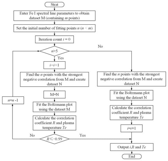
The calculation of plasma temperature is often performed using the Boltzmann plot method [30]. In this study, the plasma temperature is calculated using an improved iterative Boltzmann plot method based on the relevant parameters of 21 different characteristic spectral lines of Fe I presented in Table 4. The flowchart of this iterative algorithm is shown in Figure 15. In each iteration, the plasma electron temperature is calculated based on the slope of the linear fitting between ln(Iλ/gk/Aki) and Ek.
Table 4.
Information on characteristic spectral line correlation parameters used for calculating plasma temperature.
Taking the spectrum obtained from the 240th laser pulse as an example, the fitting results of the initial iteration and the final convergence are shown in Figure 16a, and the changes in correlation coefficient and plasma temperature during the iteration process are depicted in Figure 16b.
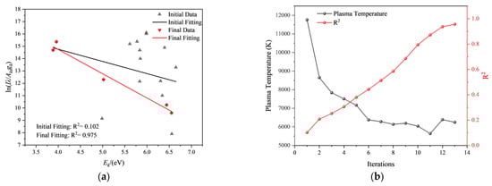
Figure 16.
Calculation process of plasma temperature for the 240th laser pulse test: (a) Fitting curves for the initial iteration and the final iteration. (b) Changes in plasma temperature and correlation coefficient during the iteration process.
It can be observed that as the number of iterations increases, the correlation coefficient gradually increases, and the plasma temperature becomes more stable. The correlation coefficient at the initial iteration is R2 = 0.102, resulting in a plasma temperature of 11,759 K. After the 6th iteration, the plasma temperature stabilizes around 6200 K. In the final iteration step, the correlation coefficient is R2 = 0.975, yielding a plasma temperature of 6249 K.
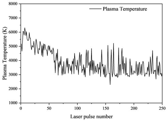
The variation in plasma temperature with laser pulse number is shown in Figure 17. It can be observed that the plasma temperature initially increases, which is because at the beginning, when the size of the ablation pit is small, the shock wave generated by the plasma expansion reflects within the pit, limiting the plasma expansion and leading to an increase in plasma temperature. However, when the depth exceeds approximately 185.42 μm (10 laser pulses), the plasma temperature gradually decreases, which is due to the fact that the sample is a composite material of fiberglass and resin, containing many pores. Heat dissipates through these pores, resulting in a decrease in temperature. Eventually, at around 270.77 μm (100 pulses), the plasma temperature fluctuates around 3500 K. This is because a balance is reached between heat dissipation and the limiting effect of the shock wave.
Plasma temperature is calculated based on the assumption of local thermodynamic equilibrium. It is necessary to assess whether the plasma is close to local thermodynamic equilibrium. The McWhirter criterion is commonly used for this assessment [31].
In the equation, Ne represents the electron number density (cm−3), and ΔE represents the maximum energy difference between the ground state and the excited state (eV).
In laser-induced plasmas, the main mechanism for the broadening of atomic emission spectral lines is Stark broadening, caused by the interaction between the emitting atoms and the surrounding charged particles’ electric fields. The electron number density can be calculated using Stark broadening [32].
In the equation, ω represents the electron collision parameter, and λ represents the Full Width at Half Maximum (FWHM) of the spectral line.
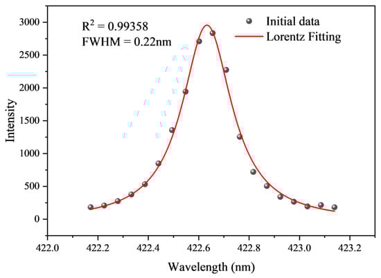
Taking Fe II 422.608 nm as an example for electron number density calculation, this spectral line is relatively independent, free from self-absorption phenomena, and has a well-defined profile. Taking the spectral data obtained from the 36th laser pulse test as an example, a Lorentzian fit was applied to the Fe II 422.608 nm spectral line, as shown in Figure 18. The fitting coefficient R2 = 0.99358 indicates an excellent fit, with a FWHM of 0.22 nm.
The approximate relationship between the electron collision coefficient ω and plasma temperature Te obtained from [33] is:
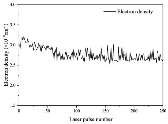
According to Equation (3), the actual electron number density is calculated and presented in Figure 19. The peak plasma temperature reaches 6311.663 K, with the energy level of Fe II at 422.608 nm being 2.933 eV. It can be deduced that the minimum electron density required to maintain local thermodynamic equilibrium is 2.806 × 1017 cm−3. The actual calculated electron density is approximately 1018 cm−3, suggesting that the plasma in this experiment is in a state of LTE. It is evident that the variation in electron density with the number of laser pulses aligns with the trend in plasma temperature, ultimately stabilizing at about 2.6 × 1018 cm−3. Furthermore, this study reveals that the changing trends of plasma temperature and electron density correspond with the fluctuations in the intensity of laser-induced plasma emission spectral lines of Fe.
4. Conclusions
In this study, the LIBS technique was employed to analyze SMC insulation material in electrical equipment. Optimal testing parameters for obtaining reliable spectral data were identified based on line intensity, SNR, and SBR. The analysis demonstrated a positive correlation between ablation depth and laser pulse number, while no correlation was observed with single laser pulse energy. The surface area of the ablation pit exhibited a strong positive correlation with both laser pulse number and single laser pulse energy. Additionally, this study compared the elemental analysis results of LIBS and EDS, revealing minor differences attributable to the low elemental content. Variations in elemental content with laser pulse number were analyzed for Na, Ti, Fe, Mg, Ca, and C. Plasma temperature and electron density in the SMC materials were calculated using Fe I and Fe II spectral lines, confirming adherence to local thermodynamic equilibrium. Overall, this study offers insights into the application of LIBS technology for testing SMC materials, highlighting the minimal sample impact from laser ablation and the precise and reliable results of LIBS analysis. These findings have significant implications for the practical use of LIBS in detecting SMC materials in electrical equipment. In the future, we will further deepen our research to carry out practical testing of SMC materials. This includes, but is not limited to, classifying SMC materials from different manufacturers, assessing the quality of SMC materials, characterizing their insulation and mechanical properties, and evaluating the degree of aging of SMC materials. In fact, we are also conducting research on the performance characterization of SMC materials, which is precisely what the technical parameters in this article are based on.
Author Contributions
Conceptualization, H.S. and H.J.; methodology, H.J.; software, H.Z.; validation, X.C., L.Y. and H.C.; formal analysis, H.S. and H.J.; investigation, T.T.; resources, X.W.; data curation, H.S.; writing—original draft preparation, H.J. and H.S.; writing—review and editing, X.W.; visualization, H.Z. and L.Y.; project administration, X.W.; funding acquisition, X.W. All authors have read and agreed to the published version of the manuscript.
Funding
This research was funded by the State Grid Shanghai Electric Power Company, grant number 52090D23000F.
Data Availability Statement
No new data were created.
Conflicts of Interest
Authors Hua Shen, Haohan Zhen, Lei Yu, Haibin Chen and Tao Tong were employed by the company State Grid Shanghai Municipal Electric Power Company Marketing Service Center. The remaining authors declare that the research was conducted in the absence of any commercial or financial relationships that could be construed as a potential conflict of interest. The authors declare that this study received funding from State Grid Shanghai Electric Power Company. The funder was not involved in the study design, collection, analysis, interpretation of data, the writing of this article or the decision to submit it for publication.
References
- Kearton, B.; Mattley, Y. Laser-Induced Breakdown Spectroscopy Sparking New Applications. Nat. Photonics 2008, 2, 537–540. [Google Scholar] [CrossRef]
- Corsi, M.; Cristoforetti, G.; Hidalgo, M. Effect of Laser-Induced Crater Depth in Laser-Induced Breakdown Spectroscopy Emission Features. Appl. Spectrosc. 2005, 59, 853–860. [Google Scholar] [CrossRef] [PubMed]
- Zheng, J.Y.; Ma, Z.; Gao, L.H. Development of intelligent anti-high power laser materials. Adv. Ceram. 2020, 41, 121–133. [Google Scholar]
- Cao, Z.; Cheng, J.; Han, X. Rapid classification of coal by laser-induced breakdown spectroscopy (LIBS) with K-nearest neighbor (KNN) chemometrics. Instrum. Sci. Technol. 2023, 51, 59–67. [Google Scholar] [CrossRef]
- Guo, H.; Cui, M.; Feng, Z. Classification of Aviation Alloys Using Laser-Induced Breakdown Spectroscopy Based on a WT-PSO-LSSVM Model. Chemosensors 2022, 10, 220. [Google Scholar] [CrossRef]
- Wang, J.; Xue, S.; Zheng, P. Determination of Lead and Copper in Ligusticum wallichii by Laser-Induced Breakdown Spectroscopy. Anal. Lett. 2017, 50, 2000–2011. [Google Scholar] [CrossRef]
- Tiwari, M.; Agrawal, R.; Pathak, A.K. Laser-Induced Breakdown Spectroscopy: An Approach to Detect Adulteration in Turmeric. Spectrosc. Lett. 2013, 46, 155–159. [Google Scholar] [CrossRef]
- Roh, S.B.; Park, S.B.; Oh, S.K. Development of intelligent sorting system realized with the aid of laser-induced breakdown spectroscopy and hybrid preprocessing algorithm-based radial basis function neural networks for recycling black plastic wastes. J. Mater. Cycles Waste Manag. 2018, 20, 1934–1949. [Google Scholar] [CrossRef]
- Ma, S.; Tang, Y.; Ma, Y. Correction: The pH effect on the detection of heavy metals in wastewater by laser-induced breakdown spectroscopy coupled with a phase transformation method. J. Anal. At. Spectrom. 2020, 35, 1499. [Google Scholar] [CrossRef]
- Rehan, I.; Gondal, M.A.; Aldakheel, R.K. Development of laser induced breakdown spectroscopy technique to study irrigation water quality impact on nutrients and toxic elements distribution in cultivated soil. Saudi J. Biol. Sci. 2021, 28, 6876–6883. [Google Scholar] [CrossRef]
- Mehari, F.; Rohde, M.; Kanawade, R. Investigation of the differentiation of ex vivo nerve and fat tissues using laser-induced breakdown spectroscopy (LIBS): Prospects for tissue-specific laser surgery. J. Biophotonics 2016, 9, 1021–1032. [Google Scholar] [CrossRef] [PubMed]
- Nouir, R.; Cherni, I.; Ghalila, H. Early diagnosis of dental pathologies by front face fluorescence (FFF) and laser-induced breakdown spectroscopy (LIBS) with principal component analysis (PCA). Instrum. Sci. Technol. 2022, 50, 465–480. [Google Scholar] [CrossRef]
- Berlo, K.; Xia, W.; Zwillich, F. Laser induced breakdown spectroscopy for the rapid detection of SARS-CoV-2 immune response in plasma. Sci. Rep. 2022, 12, 1614. [Google Scholar] [CrossRef] [PubMed]
- Poggialini, F.; Fiocco, G.; Campanella, B. Stratigraphic analysis of historical wooden samples from ancient bowed string instruments by laser induced breakdown spectroscopy. J. Cult. Herit. 2020, 44, 275–284. [Google Scholar] [CrossRef]
- Siozos, P.; Hausmann, N.; Holst, M. Application of laser-induced breakdown spectroscopy and neural networks on archaeological human bones for the discrimination of distinct individuals. J. Archaeol. Sci.-Rep. 2021, 35, 102769. [Google Scholar] [CrossRef]
- Wang, X.; Hong, X.; Chen, P. Surface Hardness Analysis of Aged Composite Insulators via Laser-Induced Plasma Spectra Characterization. IEEE T. Plasma Sci. 2019, 47, 387–394. [Google Scholar] [CrossRef]
- Wan, N.; Wang, X.; Chen, P. Metal Contamination Distribution Detection in High-Voltage Transmission Line Insulators by Laser-induced Breakdown Spectroscopy (LIBS). Sensors 2018, 18, 2623. [Google Scholar] [CrossRef] [PubMed]
- Zhang, F.; Chen, S.; Wang, T. LIBS characterization of algal fouling on insulators. J. Eng. 2021, 2021, 408–413. [Google Scholar] [CrossRef]
- Sanjana, K.; Babu, M.S.; Sarathi, R. Classification of Polluted Silicone Rubber Insulators by Using LIBS Assisted Machine Learning Techniques. IEEE Access. 2023, 11, 1752–1760. [Google Scholar] [CrossRef]
- Babu, M.S.; Neelmani; Vasa, N.J. Use of LIBS technique for identification of type of pollutant and ESDD level on epoxy-alumina nanocomposites using ANN. Meas. Sci. Technol. 2021, 32, 115201. [Google Scholar] [CrossRef]
- Gondal, M.A.; Shwehdi, M.H.; Khalil, A.A.I. Applications of LIBS for determination of ionic species (NaCl) in electrical cables for investigation of electrical breakdown. Appl. Phys. B 2011, 105, 915–922. [Google Scholar] [CrossRef]
- Neettiyath, A.; Alli, M.B.; Hayden, P. Vacuum ultraviolet laser induced breakdown spectroscopy for detecting sulfur in thermally aged transformer insulation material. Spectrochimi. Acta B 2020, 163, 105730. [Google Scholar] [CrossRef]
- Neettiyath, A.; Vasa, N.J.; Sarathi, R. Life Expectancy Estimation of Thermally Aged Cu Contaminant-Diffused Oil Impregnated Pressboard. IEEE Trans. Dielectr. Electr. Insul. 2021, 28, 637–645. [Google Scholar] [CrossRef]
- Amalanathan, A.J.; Vasa, N.J.; Harid, N. Classification of thermal ageing impact of ester fluid-impregnated pressboard material adopting LIBS. High Volt. 2021, 6, 655–664. [Google Scholar] [CrossRef]
- Yuan, H.; Ye, Z.; Wang, X. Study on spark discharge enhanced laser-induced breakdown spectroscopy of Fe particles in transformer oil. J. Anal. Atom. Spectrom. 2022, 37, 381–389. [Google Scholar] [CrossRef]
- Zhang, S.C.; Wu, L.H.; Sun, X.K. Ultra-low thermal conductivity multilayer composites for insulation in low pressure environments. Adv. Ceram. 2023, 44, 442–450. [Google Scholar]
- NIST Atomic Spectra Database Lines Form. Available online: https://physics.nist.gov/PhysRefData/ASD/lines_form.html (accessed on 6 April 2024).
- Qian, M.; Ren, C.; Wang, D. Stark broadening measurement of the electron density in an atmospheric pressure argon plasma jet with double-power electrodes. J. Appl. Phys. 2010, 107, 063303. [Google Scholar] [CrossRef]
- Stetzler, J.; Tang, S.; Chinni, R.C. Plasma Temperature and Electron Density Determination Using Laser-Induced Breakdown Spectroscopy (LIBS) in Earth’s and Mars’s Atmospheres. Atoms 2020, 8, 50. [Google Scholar] [CrossRef]
- Unnikrishnan, V.K.; Alti, K.; Kartha, V.B. Measurements of plasma temperature and electron density in laser-induced copper plasma by time-resolved spectroscopy of neutral atom and ion emissions. Pramana 2010, 74, 983–993. [Google Scholar] [CrossRef]
- Zhao, X.X.; Luo, W.F.; He, J.F. Measurements of electron number density and plasma temperature using LIBS. In Proceedings of the International Symposium on Optoelectronic Technology and Application 2016, Beijing, China, 9–11 May 2016. [Google Scholar]
- Abdellatif, G.; Imam, H. A study of the laser plasma parameters at different laser wavelengths. Spectrochimi. Acta B 2002, 57, 1155–1165. [Google Scholar] [CrossRef]
- Database for “Stark” Broadening of Isolated Lines of Atoms and Ions in the Impact Approximation. Available online: http://stark-b.obspm.fr/index.php/home (accessed on 6 April 2024).
Disclaimer/Publisher’s Note: The statements, opinions and data contained in all publications are solely those of the individual author(s) and contributor(s) and not of MDPI and/or the editor(s). MDPI and/or the editor(s) disclaim responsibility for any injury to people or property resulting from any ideas, methods, instructions or products referred to in the content. |
© 2024 by the authors. Licensee MDPI, Basel, Switzerland. This article is an open access article distributed under the terms and conditions of the Creative Commons Attribution (CC BY) license (https://creativecommons.org/licenses/by/4.0/).