

SMC Algorithms in T-Type Bidirectional Power Grid Converter

Abstract
:1. Introduction
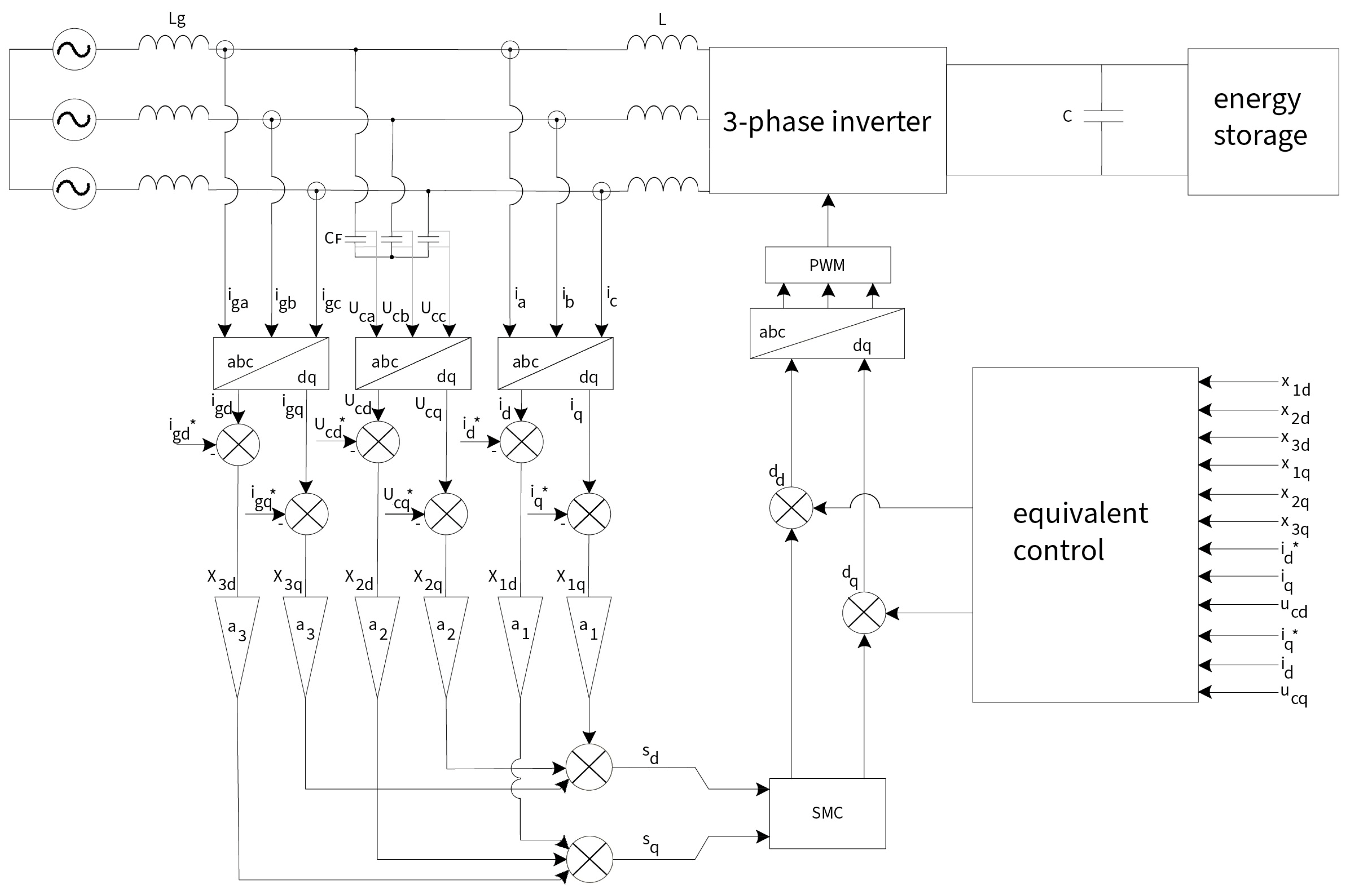
2. Methodology
- –
- —inductance of the filter on the output side of the inverter;
- –
- —output current of a given inverter phase;
- –
- —duty cycle of the voltage modulator;
- –
- —voltage on the capacitive filter on the energy storage side;
- –
- —voltage of a given phase on the capacitive filter on the power grid side;
- –
- —power grid inductance;
- –
- —power grid current of a given phase;
- –
- —power grid voltage of a given phase;
- –
- —capacity of the filter on the power grid side;
- –
- —designation of one of the three phases a, b, and c.
- –
- , —components of the output current vector of the inverter;
- –
- , —components of the duty cycle of the voltage modulator;
- –
- , —components of the voltage vector on the capacitive filter on the power grid side;
- –
- , —components of the power grid current vector;
- –
- , —components of the power grid voltage vector;
- –
- —pulsation.
- –
- , —components of the output voltage vector of the inverter.
2.1. Standard Sliding Mode Control Concept
- –
- , —sliding variables;
- –
- , , —coefficients of the sliding variable.
- Continuous part: equivalent control and reaching law;
- Discontinuous control.
- –
- —Lyapunov function for the d component of the current vector.
- –
- —the set value of the d component of the network current vector. We can determine the duty cycle signal for equivalent control of the d component:
- –
- —Lyapunov function for the q component of the current vector.
- –
- —reaching law control gain, .
- –
- , —components of the discontinuous control signal;
- –
- —gain of discontinuous control, .
2.2. Modified Sliding Mode Control Concept
- –
- , —modified reaching law controls;
- –
- , —functions implementing hybrid reaching law control;
- –
- —a parameter that is the exponent of power affecting the control gain, .
- For
- For
- –
- , —modified discontinuous controls.
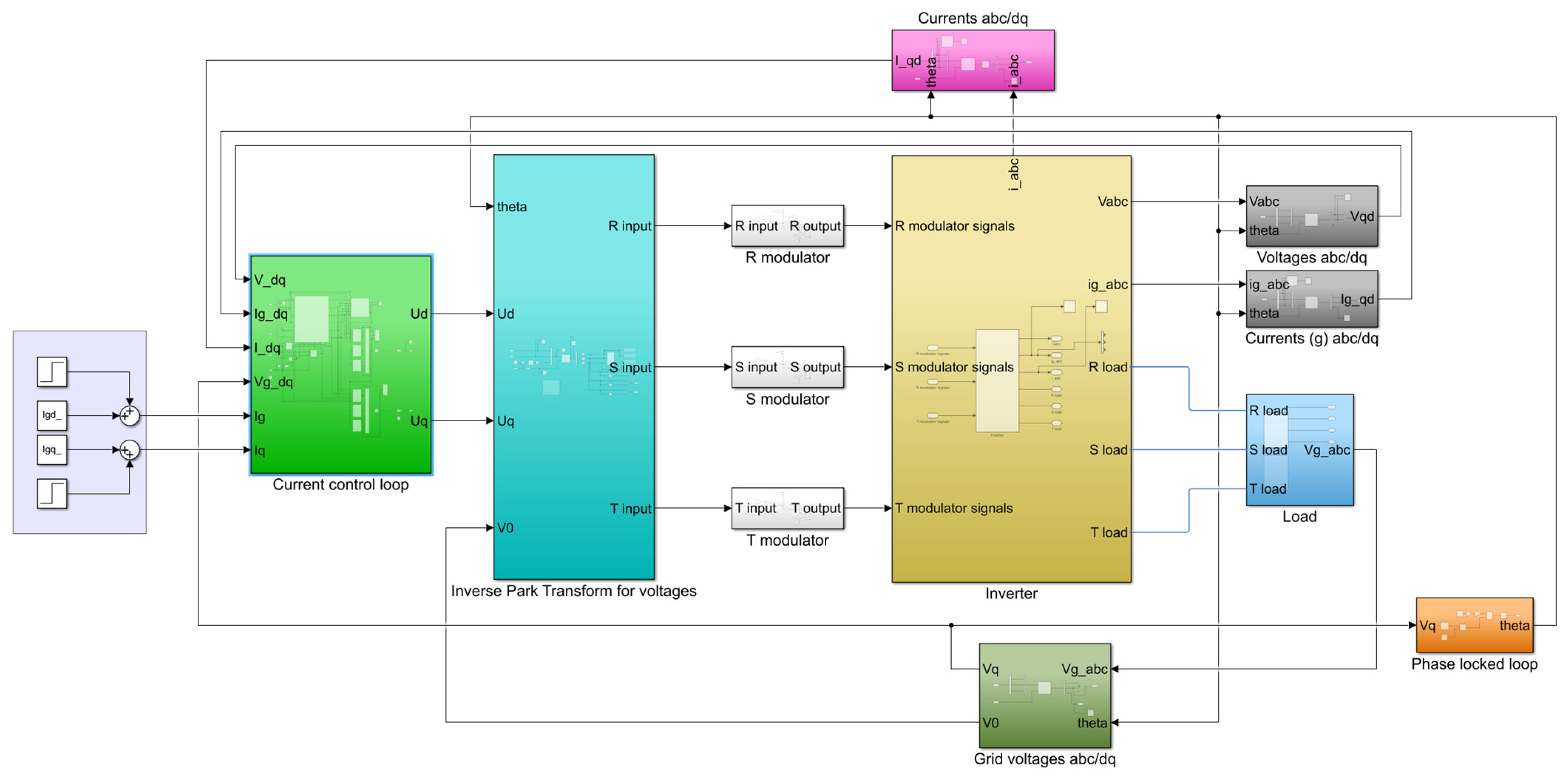
2.3. Simulation Model of T-Type Bidirectional Power Grid Converter
3. Results
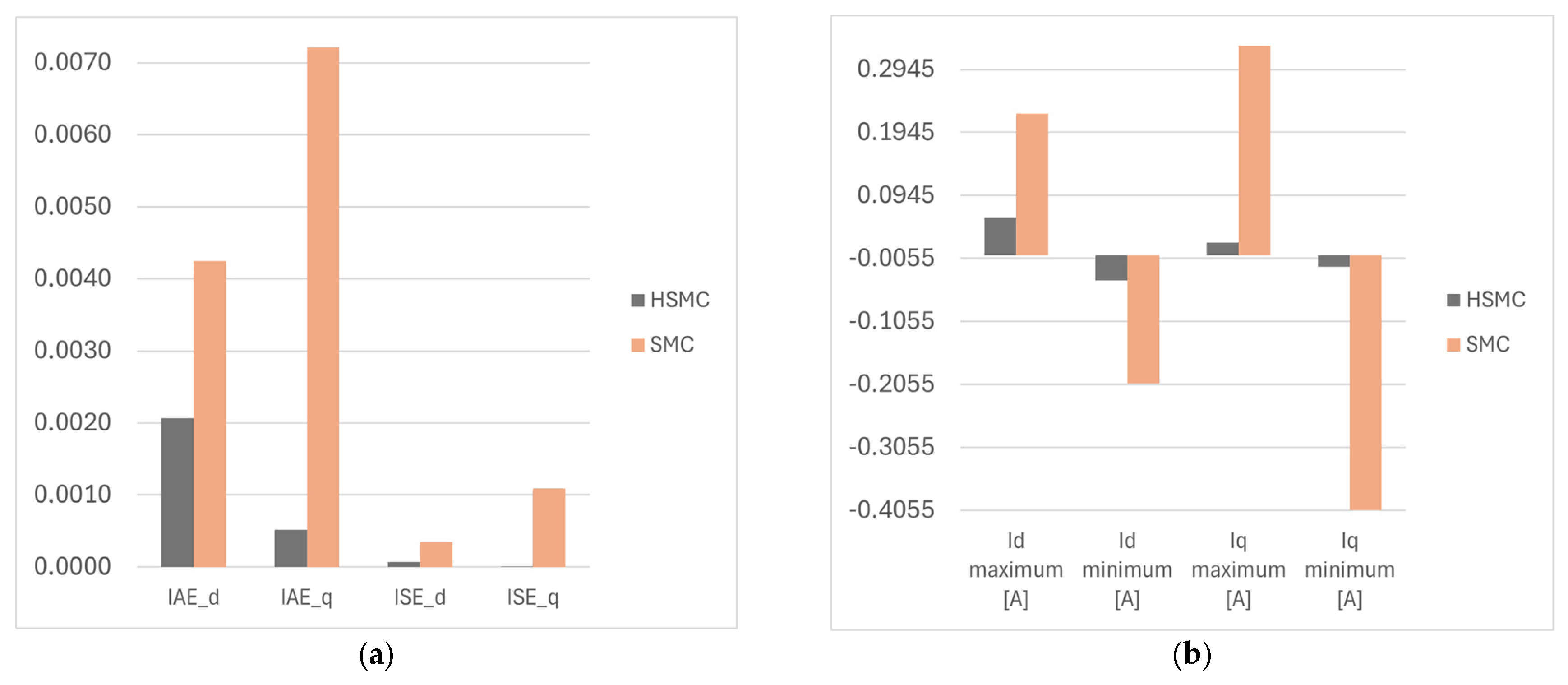
3.1. Simulation Results of SMC and Modified SMC—Static Case
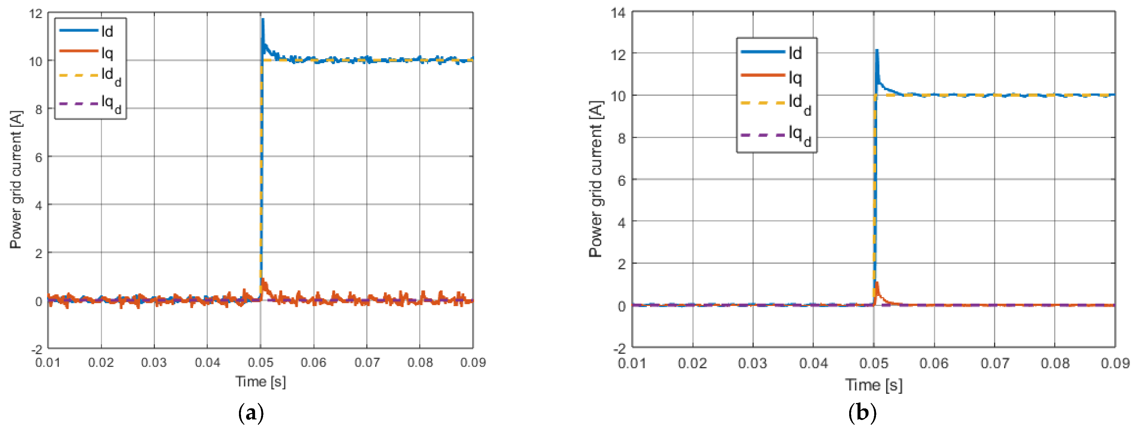
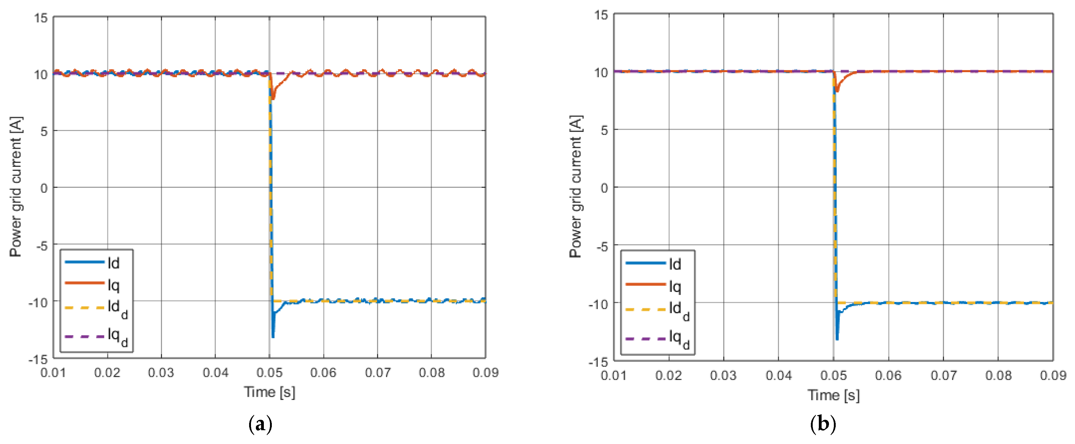
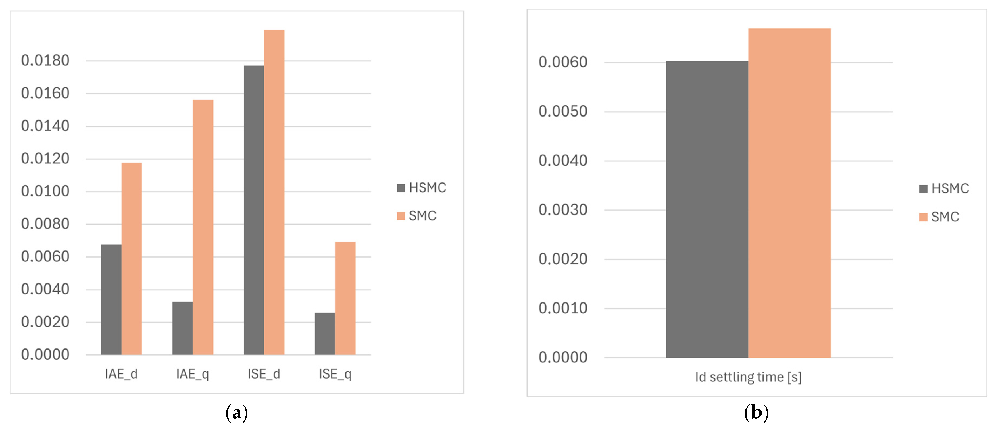
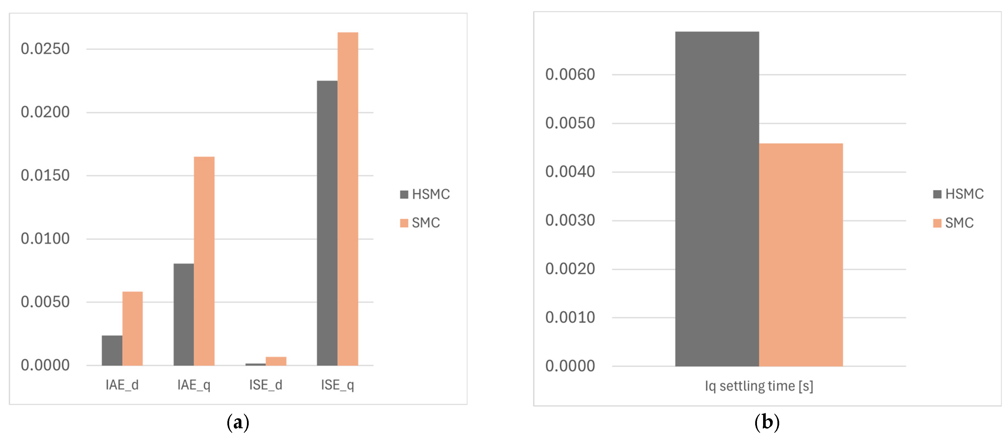
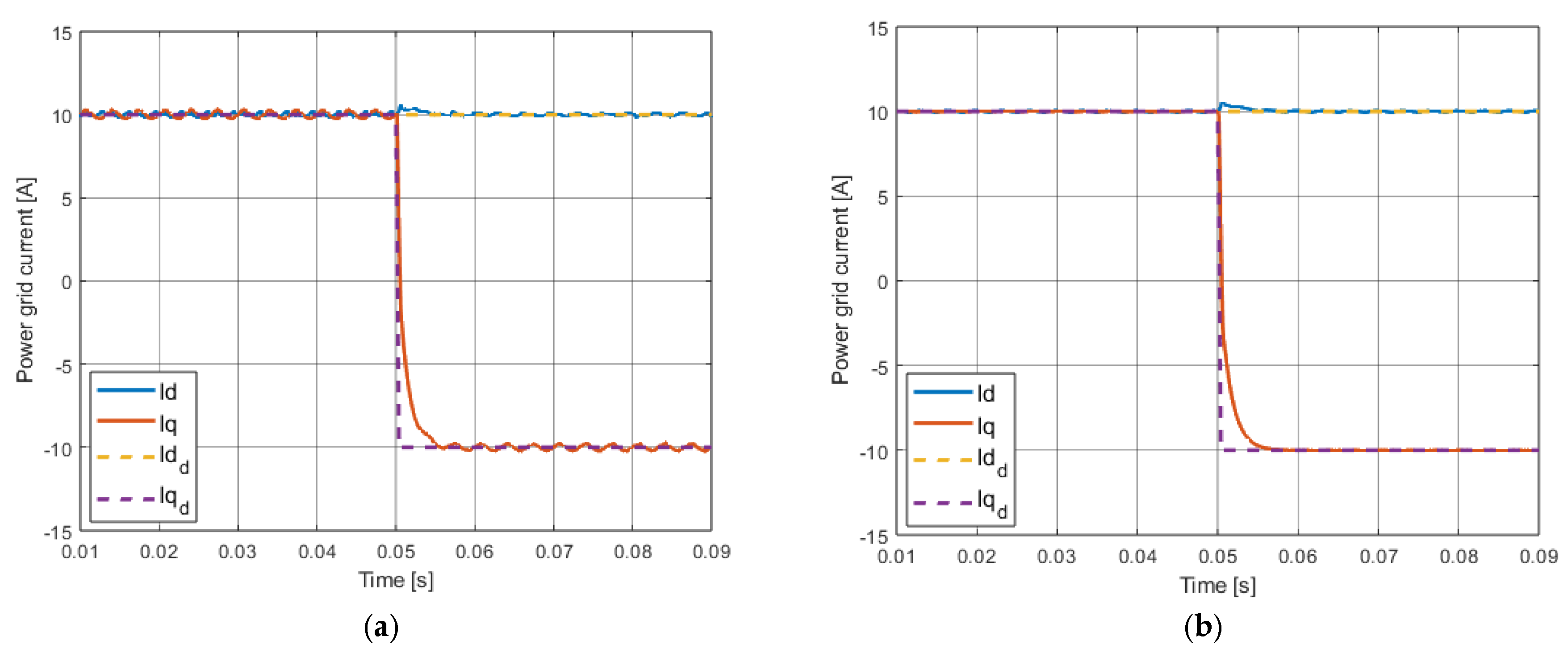
3.2. Simulation Results of SMC and Modified SMC—Dynamic Cases
- Change in from 0 to 10 A, equal to 0 A;
- Change in from 10 to −10 A, equal to 10 A;
- equal to 0 A, change from 0 to 10 A;
- equal to 10 A, change from 10 to −10 A.
4. Conclusions
Author Contributions
Funding
Data Availability Statement
Conflicts of Interest
References
- Bouzid, A.M.; Guerrero, J.M.; Cheriti, A.; Bouhamida, M.; Sicard, P.; Benghanem, M. A survey on control of electric power distributed generation systems for microgrid applications. Renew. Sustain. Energy Rev. 2015, 44, 751–766. [Google Scholar] [CrossRef]
- Rocabert, J.; Luna, A.; Blaabjerg, F.; Rodríguez, P. Control of Power Converters in AC Microgrids. IEEE Trans. Power Electron. 2012, 27, 4734–4749. [Google Scholar] [CrossRef]
- Nepal, S.; Shakya, A.; Fourney, R.; Sternhagen, J.; Tonkoski, R. Development of Real-time Control of Commercial Off-The-Shelf Inverter/Charger for Energy Management of Microgrids. In Proceedings of the 2016 IEEE Power and Energy Society General Meeting (PESGM), Boston, MA, USA, 17–21 July 2016; pp. 1–4. [Google Scholar]
- Li, S.; Zhou, S.; Li, H. Harmonic Suppression Strategy of LCL Grid-Connected PV Inverter Based on Adaptive QPR_PC Control. Electronics 2023, 12, 2282. [Google Scholar] [CrossRef]
- Huang, J.; Zhao, Y.; Wang, J.; Zhang, P. A Hybrid Active Damping Strategy for Improving the Adaptability of LCL Converter in Weak Grid. Electronics 2023, 13, 144. [Google Scholar] [CrossRef]
- Pannawan, A.; Kaewchum, T.; Saeseiw, C.; Pachanapan, P.; Hinkkanen, M.; Somkun, S. Design and Implementation of Single-Phase Grid-Connected Low-Voltage Battery Inverter for Residential Applications. Electronics 2024, 13, 1014. [Google Scholar] [CrossRef]
- Hasan, M.M.; Chowdhury, A.H. Performance Analysis of a DQ0 Controlled Grid Forming Inverter for Grid Connected Photovoltaic System: A Case Study. In Proceedings of the 2022 4th International Conference on Sustainable Technologies for Industry 4.0 (STI), Dhaka, Bangladesh, 17–18 December 2022. [Google Scholar] [CrossRef]
- Guo, W.; Mu, L. Control principles of micro-source inverters used in microgrid. Prot. Control. Mod. Power Syst. 2016, 1, 5. [Google Scholar] [CrossRef]
- Monica, P.; Kowsalya, M.; Subramanian, K. Droop Reference Based Decoupling Coupling Control of NPC Inverter for Islanded Microgrid. In Proceedings of the International Conference on Innovations in Power and Advanced Computing Technologies, Vellore, India, 21–22 April 2017; pp. 1–3. [Google Scholar]
- Heo, S.; Han, J.; Park, W. Energy Storage System with Dual Power Inverters for Islanding Operation of Microgrid. In Proceedings of the 2020 IEEE International Symposium on Circuits and Systems (ISCAS), Seville, Spain, 10–21 October 2020; pp. 1–3. [Google Scholar]
- Blackstone, B.; Hicks, C.; Gonzales, O.; Baghzouz, Y. Improved islanded operation of a diesel generator–PV microgrid with advanced inverter. In Proceedings of the 2017 IEEE 26th International Symposium on Industrial Electronics (ISIE), Edinburgh, UK, 19–21 June 2017; pp. 123–126. [Google Scholar]
- Bartoszewicz, A. Conventional Sliding Modes in Continuous and Discrete Time Domains. In Proceedings of the 2017 18th International Carpathian Control Conference (ICCC), Sinaia, Romania, 28–31 May 2017; pp. 588–590. [Google Scholar]
- Zenteno-Torres, J.; Cieslak, J.; Dávila, J.; Henry, D. Sliding Mode Control with Application to Fault-Tolerant Control: Assessment and Open Problems. Automation 2021, 2, 1–30. [Google Scholar] [CrossRef]
- Bartoszewicz, A. A new reaching law for sliding mode control of continuous time systems with constraints. Trans. Inst. Meas. Control 2014, 37, 515–521. [Google Scholar] [CrossRef]
- Volosencu, C.; Saghafinia, A. Control Theory in Engineering; IntechOpen: London, UK, 2020; pp. 101–116. [Google Scholar]
- Rajanna, G.S.; Nagaraj, H.N. Comparison between sigmoid variable reaching law and exponential reaching law for sliding mode controlled DC-DC Buck converter. In Proceedings of the 2013 International Conference on Power, Energy and Control (ICPEC), Dindigul, India, 6–8 February 2013. [Google Scholar] [CrossRef]
- Rąbkowski, J.; Kopacz, R. Extended T-type Inverter. Power Electron. Drives 2018, 3, 55–57. [Google Scholar] [CrossRef]
- Meenakshi, V.; Kavitha, M.; Santhi Mary Antony, A.; Vijeye Kaveri, V.; Radhika, S.; Godwin Immanuel, D. T-type Three Phase Inverter with Grid Connected System used in Renewable Energy Resources. In Proceedings of the International Conference on Sustainable Computing and Data Communication Systems (ICSCDS-2023), Erode, India, 23–25 March 2023; pp. 929–932. [Google Scholar]
- Choi, W.; Lee, W.; Sarlioglu, B. Effect of grid inductance on grid current quality of parallel grid-connected inverter system with output LCL filter and closed-loop control. In Proceedings of the 2016 IEEE Applied Power Electronics Conference and Exposition (APEC), Long Beach, CA, USA, 20–24 March 2016; pp. 2679–2682. [Google Scholar]
- Hao, X.; Yang, X.; Xie, R.; Huang, L.; Liu, T.; Li, Y. A fixed switching frequency integral resonant sliding mode controller for three-phase grid-connected photovoltaic inverter with LCL-filter. In Proceedings of the 2013 IEEE ECCE Asia Downunder, Melbourne, VIC, Australia, 3–6 June 2013; pp. 793–796. [Google Scholar]
- Deffaf, B.; Debdouche, N.; Benbouhenni, H.; Hamoudi, F.; Bizon, N. A New Control for Improving the Power Quality Generated by a Three-Level T-Type Inverter. Electronics 2023, 12, 2117. [Google Scholar] [CrossRef]
- Swetha, K.; Sivachidambaranathan, V. A Nonlinear Controller for Neutral Point Piloted (T-Type) Multilevel Inverter-Based Three-Phase Four-Wire DSTATCOM. Int. Trans. Electr. Energy Syst. 2022, 2022, 7899765. [Google Scholar] [CrossRef]
- Panda, S.K.; Ghosh, A. A Computational Analysis of Interfacing Converters with Advanced Control Methodologies for Microgrid Application. Technol. Econ. Smart Grids Sustain. Energy 2020, 5, 7. [Google Scholar] [CrossRef]
- Nicola, M.; Nicola, C.-I. Improved Performance in the Control of DC-DC Three-Phase Power Electronic Converter Using Fractional-Order SMC and Synergetic Controllers and RL-TD3 Agent. Fractal Fract. 2022, 6, 729. [Google Scholar] [CrossRef]
- Zhu, A.; Yu, H.; Meng, X.; Xu, T. Cooperative control of NNMPL-SMC and integral EPH methods for a class of overdamping uncertain nonlinear system. Res. Sq. 2024, 1, 2–15. [Google Scholar] [CrossRef]
- Mughees, A.; Ahmad, I. Multi-Optimization of Novel Conditioned Adaptive Barrier Function Integral Terminal SMC for Trajectory Tracking of a Quadcopter System. IEEE Access 2023, 11, 88359–88377. [Google Scholar] [CrossRef]
- Bouguerra, Z. Comparative study between PI, FLC, SMC and Fuzzy sliding mode controllers of DFIG wind turbine. J. Renew. Energies 2023, 26, 209–223. [Google Scholar] [CrossRef]
- Kalvinathan, V.; Chitra, S. Power Optimization in Hybrid Renewable Energy Standalone System using SMC-ANFIS. Adv. Electr. Comput. Eng. 2022, 22, 69–78. [Google Scholar] [CrossRef]
- Liu, S.; Liu, X.; Jiang, S.; Zhao, Z.; Wang, N.; Liang, X.; Zhang, M.; Wang, L. Application of an Improved STSMC Method to the Bidirectional DC–DC Converter in Photovoltaic DC Microgrid. Energies 2022, 15, 1636. [Google Scholar] [CrossRef]
- Leng, J.; Ma, C. Sliding Mode Control for PMSM Based on A Novel Hybrid Reaching Law. In Proceedings of the 37th Chinese Control Conference, Wuhan, China, 25–27 July 2018; pp. 3006–3009. [Google Scholar]
- Xi, L.; Dong, H.; Yang, S.; Qi, X. Terminal Sliding Mode Control for Robotic Manipulator Based on Combined Reaching Law. In Proceedings of the 2019 International Conference on Computer Network, Electronic and Automation (ICCNEA), Xi’an, China, 27–29 September 2019; pp. 436–439. [Google Scholar]
- Li, Y.; Liu, L. The research of the sliding mode control method based on improved double reaching law. In Proceedings of the 2018 Chinese Control and Decision Conference (CCDC), Shenyang, China, 9–11 June 2018; pp. 672–674. [Google Scholar]
- Mozayan, S.M.; Saad, M.; Vahedi, H.; Fortin-Blanchette, H.; Soltani, M. Sliding Mode Control of PMSG Wind Turbine Based on Enhanced Exponential Reaching Law. IEEE Trans. Ind. Electron. 2016, 63, 6148–6159. [Google Scholar] [CrossRef]
- Schonardie, M.F.; Coelho, R.F.; Schweitzer, R.; Martins, D.C. Control of the Active and Reactive Power Using dq0 Transformation in Three-Phase Grid-Connected PV System. In Proceedings of the 2012 IEEE International Symposium on Industrial Electronics, Hangzhou, China, 28–31 May 2012; pp. 264–266. [Google Scholar]
- Vinoliney, A.; Lydia, M.; Levron, Y. Optimal grid integration of renewable energy sources with energy storage using dq0 based inverter controller. In Proceedings of the 2020 International Conference on Inventive Computation Technologies (ICICT), Coimbatore, India, 26–28 February 2020; pp. 966–968. [Google Scholar]
- Zargari, N.; Ofir, R.; Levron, Y.; Belikov, J. Using DQ0 Signals based on the Central Angle Reference Frame to Model the Dynamics of Large-scale Power Systems. In Proceedings of the 2020 IEEE PES Innovative Smart Grid Technologies Europe (ISGT-Europe), The Hague, The Netherlands, 26–28 October 2020. [Google Scholar] [CrossRef]
- Xu, S.; Zhang, J.; Hang, J. Investigation of a fault-tolerant three-level T-type inverter system. In Proceedings of the 2015 IEEE Energy Conversion Congress and Exposition (ECCE), Montreal, QC, Canada, 20–24 September 2015. [Google Scholar] [CrossRef]
- Han, Y.; Yang, M.; Li, H.; Yang, P.; Xu, L.; Coelho, E.A.A.; Guerrero, J.M. Modeling and Stability Analysis of LCL-Type Grid-Connected Inverters: A Comprehensive Overview. IEEE Access 2019, 7, 114975–115001. [Google Scholar] [CrossRef]
- Zheng, C.; Liu, Y.; Liu, S.; Li, Q.; Dai, S.; Tang, Y.; Zhang, B.; Mao, M. An Integrated Design Approach for LCL-Type Inverter to Improve Its Adaptation in Weak Grid. Energies 2019, 12, 2637. [Google Scholar] [CrossRef]
- Wang, X.; Wang, D.; Zhou, S. A Control Strategy of LCL-Type Grid-Connected Inverters for Improving the Stability and Harmonic Suppression Capability. Machines 2022, 10, 1027. [Google Scholar] [CrossRef]
- Aapro, A.; Messo, T.; Suntio, T. Effect of active damping on the output impedance of PV inverter. In Proceedings of the 2015 IEEE 16th Workshop on Control and Modeling for Power Electronics (COMPEL), Vancouver, BC, Canada, 12–15 July 2015. [Google Scholar] [CrossRef]
- Utkin, V.; Shi, J. Integral Sliding Mode in Systems Operating under Uncertainty Conditions. In Proceedings of the 35th IEEE Conference on Decision and Control, Kobe, Japan, 13 December 1996; pp. 4591–4593. [Google Scholar]


| Name of the Parameter | Value |
|---|---|
| Simulation time step | 100 ns |
| Modulator frequency | 50 kHz |
| DC source voltage | 350 V |
| Filter inductance (inverter output side) | 1.4 mH |
| Filter capacitance | 0.2 mF |
| Filter inductance (load side) | 0.127 mH |
| Cases | IAE_d | IAE_q | ISE_d | ISE_q |
|---|---|---|---|---|
| Static case (SMC) | 0.0042 | 0.0072 | 0.0004 | 0.0011 |
| Static case (HSMC) | 0.0021 | 0.0005 | 0.0001 | 0.000005 |
| Cases | Maximum [A] | Minimum [A] | Maximum [A] | Minimum [A] |
|---|---|---|---|---|
| Static case (SMC) | 0.2247 | −0.2039 | 0.3326 | −0.4055 |
| Static case (HSMC) | 0.0599 | −0.0411 | 0.0199 | −0.0184 |
| Cases | IAE_d | IAE_q | ISE_d | ISE_q |
|---|---|---|---|---|
| : from 0 to 10 A (SMC) | 0.0066 | 0.0079 | 0.0079 | 0.0015 |
| : from 0 to 10 A (HSMC) | 0.0051 | 0.0019 | 0.0112 | 0.0006 |
| : from 10 to −10 A (SMC) | 0.0118 | 0.0156 | 0.0199 | 0.0069 |
| : from 10 to −10 A (HSMC) | 0.0068 | 0.0032 | 0.0177 | 0.0026 |
| : from 0 to 10 A (SMC) | 0.0059 | 0.0165 | 0.0007 | 0.0263 |
| : from 0 to 10 A (HSMC) | 0.0024 | 0.0081 | 0.0002 | 0.0225 |
| : from 10 to −10 A (SMC) | 0.0068 | 0.0259 | 0.0010 | 0.0956 |
| : from 10 to −10 A (HSMC) | 0.0032 | 0.0153 | 0.0004 | 0.0824 |
| Cases | Settling Time [s] | Settling Time [s] |
|---|---|---|
| : from 0 to 10 A (SMC) | 0.0042 | - |
| : from 0 to 10 A (HSMC) | 0.0047 | - |
| : from 10 to −10 A (SMC) | 0.0067 | - |
| : from 10 to −10 A (HSMC) | 0.0060 | - |
| : from 0 to 10 A (SMC) | - | 0.0046 |
| : from 0 to 10 A (HSMC) | - | 0.0069 |
| : from 10 to −10 A (SMC) | - | 0.0057 |
| : from 10 to −10 A (HSMC) | - | 0.0081 |
Disclaimer/Publisher’s Note: The statements, opinions and data contained in all publications are solely those of the individual author(s) and contributor(s) and not of MDPI and/or the editor(s). MDPI and/or the editor(s) disclaim responsibility for any injury to people or property resulting from any ideas, methods, instructions or products referred to in the content. |
© 2024 by the authors. Licensee MDPI, Basel, Switzerland. This article is an open access article distributed under the terms and conditions of the Creative Commons Attribution (CC BY) license (https://creativecommons.org/licenses/by/4.0/).
Share and Cite
Sawiński, A.; Chudzik, P.; Tatar, K. SMC Algorithms in T-Type Bidirectional Power Grid Converter. Energies 2024, 17, 2970. https://doi.org/10.3390/en17122970
Sawiński A, Chudzik P, Tatar K. SMC Algorithms in T-Type Bidirectional Power Grid Converter. Energies. 2024; 17(12):2970. https://doi.org/10.3390/en17122970
Chicago/Turabian StyleSawiński, Albert, Piotr Chudzik, and Karol Tatar. 2024. "SMC Algorithms in T-Type Bidirectional Power Grid Converter" Energies 17, no. 12: 2970. https://doi.org/10.3390/en17122970