Abstract
Australia, like many other countries around the world, is undergoing a transition toward net zero emissions. It requires changes and development in many sectors, which not only bring benefits but also challenges. The rapid growth in renewable energy sources (RESs) is necessary to decarbonise electricity generation but negatively affects grid stability. Residential buildings also contribute to this issue through specific load profiles and the high penetration of rooftop photovoltaic (PV) installations. Maintaining grid balance will be crucial for further emissions reductions. One of the potential solutions can be the replacement of conventional heating and cooling systems in houses with solutions capable of storing energy and shifting the electrical load. As presented in this paper, heat pumps and hydronic systems can significantly improve the electrical load of a typical South Australian household when they are controlled by algorithms reacting to the current grid conditions and household-generated electricity compared to conventional solutions. TRNSYS 18 simulations of air source and ground source heat pump systems with smart control based on measured electricity consumption and domestic hot water usage data showed the possibility of total energy consumption reduction, shifting the load from peak periods towards periods of excessive RES generation and increasing self-consumption of rooftop PV electricity. These improvements reduce the amount of emissions generated by such a household and allow for further development of other sectors.
1. Introduction
Australia fulfilled its 2020 carbon emissions plans and is on track to meet the 2050 goal of reaching net zero emissions [1]. However, it requires multifield improvements. Among the affected sectors is electricity generation, with a modelled reduction in emissions of up to 97% compared to 2005 [1]. This is to be achieved mainly by an enormous increase in the contribution of RESs. Another affected sector is Australian buildings, including residential ones, which account for over 10% of Australia’s current carbon emissions [2]. These two sectors are connected by the electrical grid, which also needs to undergo changes to adapt to new, less carbon-emission-dependent realities.
Most Australian residences are connected to the grid operated by the Australian Energy Market Operator (AEMO). The Australian National Electricity Market (NEM) is one of the longest interconnected electricity grids in the world (about 5000 km), covering six out of eight Australian states (Queensland, New South Wales, Australian Capital Territory, Victoria, South Australia and Tasmania) [3]. AEMO allows for trading and exchanging energy between regions to meet the demand in every part of the grid. AEMO is also responsible for demand prediction and maintaining the necessary level of reserves [4]. However, these tasks are becoming more and more difficult due to reasons such as the increasing penetration of RESs and the peak demand phenomenon. According to ENERGEIA forecasts, issues such as instabilities in demand and complexity of electricity generation control will become more challenging in the following decades [5].
Grid stability is a cornerstone of a well-functioning electrical power system, which is indispensable in modern society. An imbalance between electricity generation and demand can lead to voltage and frequency deviations, potentially causing equipment damage and disruptions in the power supply. Moreover, grid instability can result in blackouts or brownouts, negatively impacting both residential and industrial consumers. Australia is currently confronted with issues related to grid instability, and the problem is likely to worsen [6]. This contradicts one of the key principles of Australia’s Long-Term Emissions Reduction Plan, which mentions providing reliable power [1]. Therefore, the implementation of increased grid-preserving technologies is required.
1.1. Residential Electrical Load
The residential sector is a significant contributor to grid stress [7]. Specific consumption profiles and increasing decentralised electricity generation cause demand and supply instability. These problems also concern the Australian National Grid. One of the contributors to grid imbalance is the high penetration of rooftop PV systems, which causes excess and uncontrollable generation. Australia is the world leader in rooftop PV systems, and around 35% of Australian households have installed a solar PV system, with states such as Queensland and South Australia reaching the level of about 45% [8]. The other contributor is a fluctuating load of heating and cooling devices due to weather conditions and residents’ behaviour patterns. The number of small and medium reverse-cycle air conditioners, which are typical for the residential market, is increasing [9]. This creates additional load, especially during extreme weather events. This trend is likely to continue due to decarbonisation and electrification of heating [10] and increasing cooling and dehumidification demand [11].
Therefore, many research considerations are focused on improvements in energy consumption in the housing sector. Most proposed solutions are concerned with increasing rooftop PV generation self-consumption and demand-response programs. The desirable result would be shifting the load from peak hours to periods with the highest PV generation. This would help to utilise carbon emission-free energy instead of other energy sources, including fossil-based generators. As the major contributors to household energy consumption, space conditioning and water heating [8] are the main factors affecting the residential electricity load profile. Therefore, many researchers have investigated the possibility of adapting air conditioners and domestic hot water (DHW) heaters in the smart grid to address the demand response in Australia.
1.2. Current Solutions
The factors mentioned above necessitate the introduction of new solutions, such as smart management. The smart grid allows for detecting and reacting to changes in electricity demand and fluctuations in RES output using a digital communication network [12]. All the receivers and generators are connected to the network and monitored in real time, and if necessary, the grid operator can introduce appropriate actions. Smart management is based on the Internet of Things (IoT) concept, which relies on interconnections of various devices and objects over the global network to allow them to exchange data and interact all the time [13]. Therefore, the IoT opens new possibilities for measuring, understanding, and controlling more and more complex demand and supply phenomena.
Numerous research programs have proved that IoT has great potential in managing residential peak demand [13,14,15]. Australia has already implemented or is still implementing IoT and smart management solutions, beginning from the most basic, such as controlled load. This is a separate circuit powering large receivers, such as hot water heaters or pool filtration and heat pump systems, which is only activated during off-peak hours [16]. Another more complex and flexible solution is remote limiting or turning off large devices if the grid struggles with too high demand. An example of this system is the PeakSmart air conditioning program, where consumers agree to add a remote control to their air conditioners in exchange for a reward. If the grid experiences unusually high peak demand, the AC unit output can be limited, or the device can be completely turned off until the peak drops [17]. Finally, some programs analyse the entire household’s energy consumption and production and suggest when is the best time to use electric appliances or when it is desired not to use them. An example of this solution is granted by the SA government EmberPuls program [18]. It offers energy usage and production analysis, operation cost optimisation suggestions, and remote control of various electric circuits (appliances) in a household.
Unfortunately, most of these solutions have a major disadvantage. They require changes in the behaviour patterns of users and affect their comfort. This is especially noticeable when controlling AC load. Residential AC is one of the major contributors to peak demand events, particularly on extremely hot or cold days [19]. Therefore, the demand-response programs usually limit AC load when it is the most needed. Due to the low heat capacity of air, the lack of air conditioning is quickly apparent, causing aversion to these types of programs among the population.
Another approach to stabilise residential electrical load is transitioning towards the self-consumption of energy produced from a rooftop PV system proposed in many studies [20,21,22]. The considerations contain conclusions indicating financial (reducing bills), technical (decreasing grid load), and environmental (reduced carbon emission) benefits. However, they also mention the need to have batteries to store energy. Due to variability in PV generation that does not coincide with residential electricity demand, it is necessary to store exceeded energy to be able to use it later. Therefore, instead of pushing electricity to the grid during midday and contributing to afternoon peak demand, charging batteries while the generation is too high to use stored energy later would be more desirable.
Nevertheless, some researchers warn against the limited lifetime, dangerous materials used for production, energy-consuming production, and costly recycling of batteries, and they suggest considering other solutions to store energy [22]. This fact should be taken into account to mitigate environmental or health problems. Another issue causing a hurdle for battery storage adoption is the cost of the system, which is still high.
1.3. Heat Pumps in Grid Stabilisation
Heat pumps are also refrigeration devices, such as AC. However, they require a hydronic system to transfer heat energy. Hydronic systems use water as an additional medium to distribute thermal energy in the building. There are two types of residential heat pumps. An air source heat pump (ASHP), similar to AC, uses outside air as one of the reservoirs, whereas a ground source heat pump (GSHP) uses the ground to collect or dump heat [23]. Hydronic systems are also found in many variants. The most common solutions for heating are hydronic underfloor heating (HUFH) and radiators, whereas a hydronic fan coil unit allows for both heating and cooling. The hydronic system can also prepare DHW. An additional heat exchanger is necessary for this task because a hydronic system is a closed circuit and cannot mix with drinking water. For domestic applications, this is usually a DHW tank with a coil inside, which is heated by circulating hydronic system water. Another common part of the system is a buffer tank, which, among other tasks, allows for the accumulation of thermal energy. Therefore, it is often named as thermal energy storage (TES). It also allows for the separation of a heat pump from the space conditioning system. Thanks to that, both parts of the system can work independently, as long as the water temperature in the buffer tank is in the operating range of a heat pump and still allows for conditioning (is colder or warmer than the conditioned space).
Storage ability and independent heat pump and distribution system operation are desirable for smart grid management [24]. It allows for controlling the heat pump output without disturbing the indoor temperature, maintaining constant thermal comfort [24]. According to simulations from Spain [25], heat pumps can provide heat reserve during electricity overproduction time, consuming problematic surplus. A hydronic system can accumulate it, delivering only the required heat to the conditioned rooms. Moreover, a heat pump can be turned off, or its output can be tempered, during peak hours, reducing the grid load while the building is still conditioned by energy stored in water. Therefore, hydronic systems with heat pumps would be much more suitable for stabilising the residential load than conventional solutions. Heat pumps with TESs tend to affect users’ comfort much less than AC when their load is adjusted to the current grid needs. They also do not use as many dangerous and environmentally affecting materials as battery systems.
The importance of heat pumps in smart grid management has been studied in numerous research works, which can be categorised into three groups regarding the approach: grid-focused, price-focused, and renewable-energy-focused [24]. An example of grid-focused research is presented in a study from Germany that explores the high penetration of PV with and without heat pump integration [26]. The results show fewer critical grid parameters under high penetration of heat pumps. A study from Denmark, in turn, aims at the dynamic pricing of electricity, which corresponds to the grid’s conditions [27]. This type monitors the current electricity price, which reflects the supply–demand ratio. When there is too much supply, the price is low to encourage customers to use more energy. When the grid suffers from insufficient generation, the price rises to promote a reduction in consumption. Heat pumps under price-reacting management helped to keep the grid under grid load limits even during critical scenarios. Continuing, the problem with increasing fluctuations in Ireland’s grid caused by the growing penetration of wind power resulted in an investigation of electrification of residential heating as a solution [28]. According to the results, 20% of national domestic heat demand delivered by heat pumps with thermal storage would add only 3% CO2 emissions by the electricity sector, simultaneously decreasing much more pollution from fuel burning. Moreover, storage allows for reducing peak demand and influences the flattening load profile. These research projects, mainly from Europe and the U.S., demonstrate that hydronic heating and cooling systems based on heat pumps have a huge potential for application as a tool in smart grid management.
Unfortunately, heat pumps and hydronic systems are not popular in Australia due to the lack of awareness among builders and house owners, the complexity of the system, and higher than conventional system investment costs. Therefore, their potential for stabilising the Australian grid has not been adequately investigated. One of the few studies was conducted at RMIT University in Melbourne, where the authors analysed the usage of an air source heat pump and thermal storage to deliver DHW, heating, and cooling while utilising rooftop PV energy and decreasing peak loads [29,30]. The simulations conducted for a representative Australian house located in Brisbane and equipped with a 5 kW PV installation showed 76% potential to reduce annual grid load compared with a system without thermal storage. Moreover, the results showed the potential to decrease peak load by approximately 45% and increase solar energy self-consumption to 56%. Nevertheless, the study had some limitations. First of all, the model only took rooftop PV generation into consideration and did not react to grid conditions. Secondly, the model used very simplified occupancy and behaviour patterns. Lastly, the air source heat pump used in their model is typical for commercial installations, not residential systems.
Therefore, it has been decided to investigate the potential of hydronic heat pump systems with smart management in flattening the residential electrical demand and generation, which will be crucial in the ongoing transition towards net zero carbon emission. The study presented in this paper focused on analysing the impact of such systems in a typical South Australian household compared to conventional solutions.
2. Study
The major part of the study was designing and conducting TRNSYS simulations. Their goal was to allow a comparison of electricity consumption profiles in a typical South Australian household between a conventional system with reverse-cycle air conditioning coupled with an electric water heater and a hydronic heat pump system for space conditioning and DHW preparation. Two heat pump types were investigated: ASHP and GSHP. Heat pump operation was controlled by a standard or a smart control strategy. The second one focused on adjusting heat pump output to the current grid condition and surplus PV generation. The current grid conditions were determined based on the wholesale electricity price. The simulations were performed for the Adelaide location for a year’s duration. The TRNSYS timestep was set to 1 min to ensure high accuracy of the calculations. However, input and result data timesteps were set to 30 min. Any later-mentioned timesteps refer to 30 min intervals.
2.1. TRNSYS Model and Input Data
The study was based on the electricity consumption and PV generation load of dozens of Adelaide households measured by the Commonwealth Scientific and Industrial Research Organisation (CSIRO) [31]. Monitoring was conducted from 2012 to 2017. The averaged data from 39 households was collected from various circuits with a 30 min resolution. Due to the significant drop in the number of households participating in the program in the second half of 2017, it was decided to use data from 2016. Table 1 presents the electricity consumption and generation used in the study. Due to the size of the data, the table contains only total annual values for PV generation, AC load, and remaining load. The remaining load is a sum of all other circuits, excluding AC and DHW. DHW load was excluded due to the fact that some of the houses were equipped with a gas DHW heater, which could distort the results.

Table 1.
Total annual load of a typical South Australian household from CSIRO study.
An AC electricity load constituted the consumption of the conventional space conditioning system for the rest of the study. Similar to the previously presented case for Queensland [32], the electric load was used to calculate a typical household space conditioning thermal load. The electricity consumption of the reverse-cycle air conditioning unit and its thermal energy capacity are relative to indoor and outdoor conditions. Knowing the electricity power P and using a coefficient of performance at specific outdoor temperatures COPT of the popular middle-range split air conditioner series [33], it was possible to estimate the thermal load Q produced by the AC using the equation below:
The required weather data for the analysed year were acquired from Meteostat [34], while indoor conditions were assumed to be constant: 24 °C and 55% relative humidity for the cooling season and 21 °C for the heating season. Another assumption was that days with a mean ambient temperature <18 °C were heating days, and ≥18 °C were cooling days. This process allowed for the creation of house heating and cooling loads, which are affected not only by weather conditions and building properties but also by behaviour patterns and user preferences. The peak cooling load reached 5 kW, while the peak heating load was 2.8 kW. The loads are relatively low. However, it needs to be remembered that this is an average load of 39 households.
As explained earlier, a DHW load for the conventional solution had to be produced. The measured data from another study allowed for the preparation of a daily DHW usage profile [35] to represent typical household usage accurately. This load was then loaded to a simple TRNSYS simulation of a 200l electric water heater to create an electricity consumption profile of conventional DHW heating.
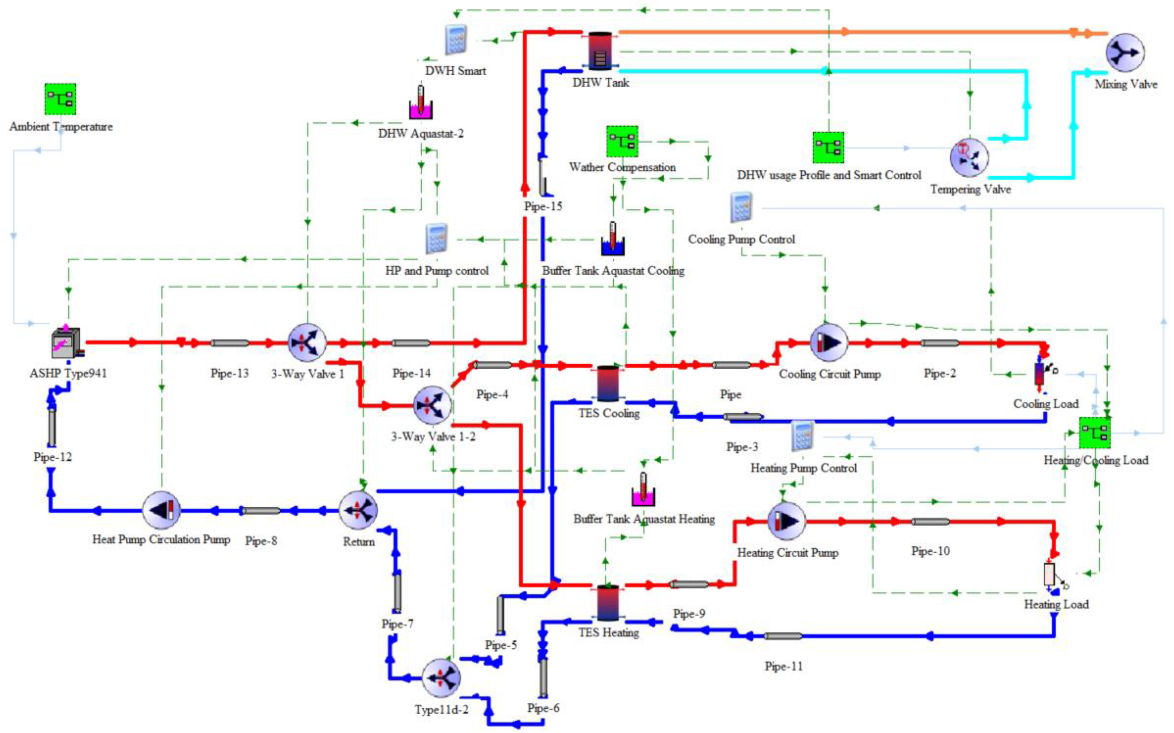
The TRNSYS model of a hydronic system was composed of the following components:
- ASHP with implemented weather data or GSHP with implemented GHX model;
- 200l DHW tank with outlet equipped with a tempering valve set to 50 °C;
- 350l TES for cooling;
- 250l TES for heating;
- Pumps, piping, and valves;
- DHW, heating and cooling circuits imposing load;
- Control system components.
Performance data of the heat pumps were modelled based on real devices available locally or in nearby markets. The GSHP was modelled according to Ecoforest ecoGEO+ 1–9 [36] performance. The TRNSYS ground source heat pump component is single-speed. Therefore, only data for the maximum output was considered. However, due to the capacity of GSHP significantly exceeding the peak loads, 60% of heating and cooling outputs were assumed, reaching 6.54 kW for both. Electricity power was accordingly adjusted. The GSHP was connected to a 110 m vertical ground heat exchanger. The model of the ASHP was based on the performance of a Mitsubishi Electric PUHZ-SHW 80VAA/YAA [37]. Similar to the GSHP, the TRNSYS component from the ASHP is single-speed. However, the performance of the ASHP is highly dependent on the outdoor temperature, and therefore, most typical residential devices are variable-speed. To mirror this for cooling, the performance data for various outdoor temperatures are modelled for different compressor speeds; the hotter the ambient temperature, the higher the compressor speed used. Due to the heating load being significantly lower than the cooling, only the middle compressor speed was used. As previously for the GSHP, the output was scaled to match the household space conditioning load. This time, it was 80% of the capacity, which reached 5.12 kW for heating and 5.68 kW for cooling. TES tank sizes were determined using Equation (2), recommended by various manufacturers [38], and rounded to the nearest commonly available sizes.
The model’s operation principle is that the heat pump provides heating or cooling to one of the tanks. For space conditioning, it is a TES heating or a TES cooling tank, while the hot water system is a DHW tank. The tanks’ temperatures are maintained according to the strategy further described and kept within the hysteresis sets. Discharging of the tanks is then conducted by another circuit connected to each of them. This allows for the independent operation of the heat pump and DHW, as well as heating and cooling circuits. All of the main components are presented in Figure 1.
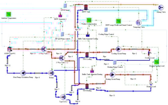
Figure 1.
TRNSYS model of the hydronic system based on ASHP.
2.2. Electricity Trading Price as a Grid Condition Indicator
The model required an indicator of whether the grid is well balanced or if it suffers from overgeneration or insufficient generation. Electricity trading prices are a good index of the grid condition. The price drops when the electricity demand is low, or generation is too high. Meanwhile, high demand or insufficient generation makes the prices rise. The Australian Energy Market Operator (AEMO) shares and archives the electricity trading prices and total demand on its website [39]. The data were acquired and processed to meet the model’s needs. It was necessary for the model to use the price for 2016 to ensure that all of the inputs (energy consumption and generation, weather data, and electricity price) aligned and presented the same events, such as peak load periods during hot days. The price was divided into five categories, with the lowest referring to extreme overgeneration and the highest referring to extreme peak demand. The price ranges for each category are presented in Table 2.
Table 2.
SA electricity price in AUD/MWh divided into five categories
2.3. Control Strategies
Control strategies were based on the systems typical in residential heat pumps. The heat pump prioritises DHW preparation over space conditioning. Therefore, whenever DHW aquastat calls DHW tank heating, the heat pump is turned on or switched from another mode and starts domestic hot water tank heating until the aquastat is satisfied. When the DHW tank temperature is satisfied, the heat pump can switch to supply TES heating or TES cooling tanks. Both TES tanks’ temperatures are maintained according to the weather compensation (heating and cooling curves). This allows for adjustment of the temperature in the TES tanks according to the outdoor temperature. Weather compensation is commonly used in this type of system to increase efficiency [40].
2.3.1. Standard Control Strategy
A standard control strategy was created to allow a direct comparison between a conventional and a hydronic system. This strategy does not include any components focused on matching the grid needs or increasing the self-consumption of household-generated PV electricity. This step also allowed for the determination of whether any positive or negative impact on the grid was due to hydronic system properties or smart strategies.
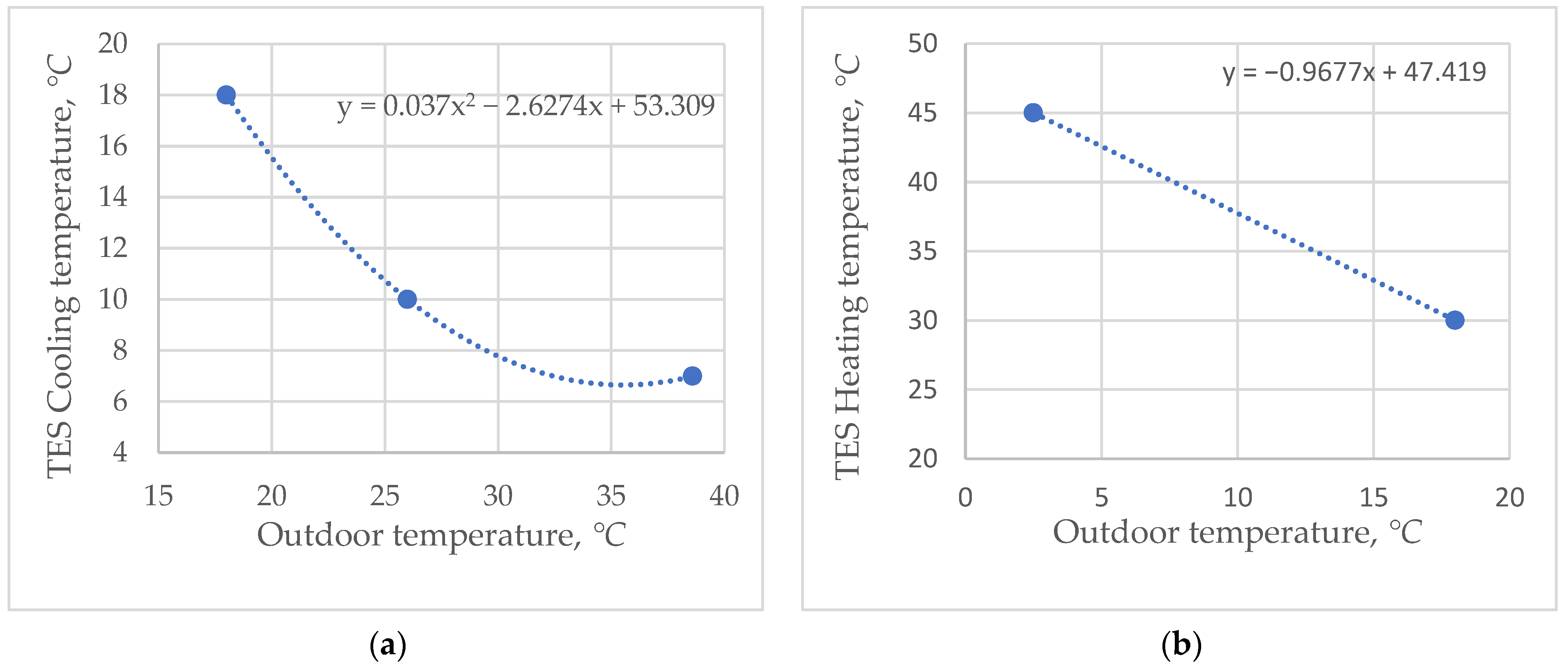
This control strategy assumes a fixed DHW tank temperature of 57 °C with 6 °C hysteresis. The weather compensation curve for cooling was created in such a way that for the hottest timestep of the analysed year, the TES cooling temperature was 7 °C. When the outdoor temperature reaches 18 °C, which is the cooling and heating mode boundary value, the TES cooling temperature is 18 °C. It was assumed that the system was equipped with a hydronic fan coil with a cooling capacity for 7 °C entering water temperature, which exceeds the peak cooling load by 25%. It turned out that a linear characteristic was not sufficient to provide enough cooling capacity in the middle of the range. Therefore, an additional point was added to create a quadratic characteristic.
The heating curve was created using the same methodology. For the coldest timestep, the TES heating tank is heated to 45 °C, whereas for 18 °C outdoor, the tank temperature set is 30 °C. For simplification purposes, it was assumed that the heating system uses the same hydronic fan coil as for cooling. In this case, a linear characteristic turned out to be sufficient. Weather compensation for heating and cooling are presented in Figure 2. Both aquastats for TES tanks were also programmed to work with 2 °C hysteresis.
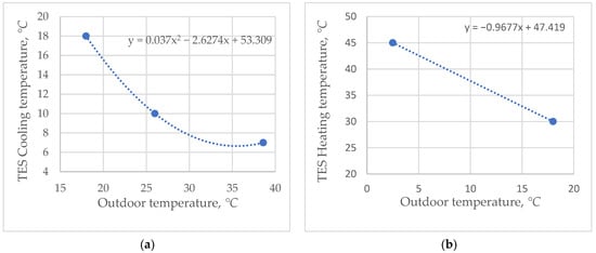
Figure 2.
Weather compensation for (a) cooling and (b) heating.
2.3.2. Smart Control Strategy (Price Only)
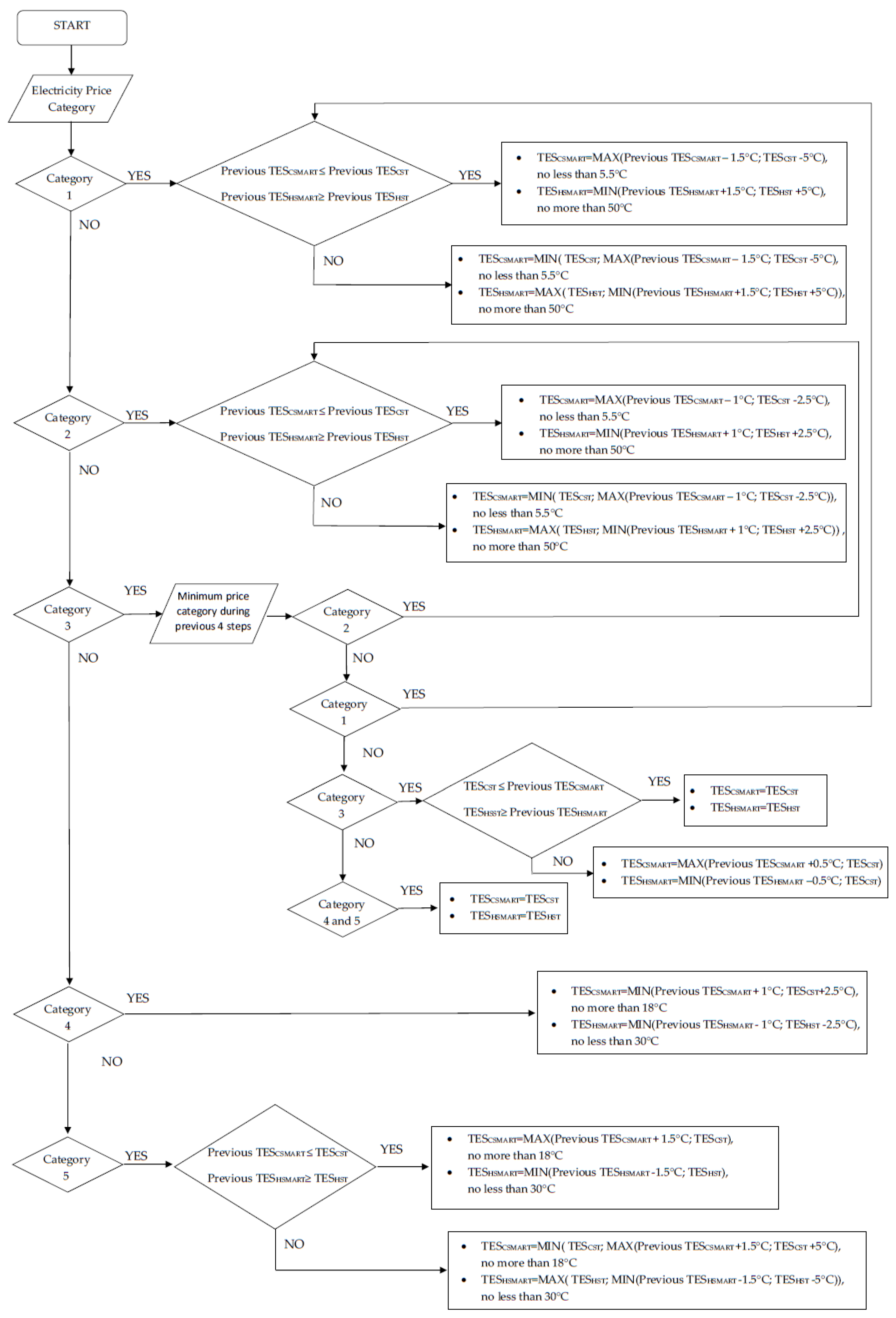
A smart control strategy was created based on a standard control strategy. The first version of smart control used only price categories to shift the electricity load from periods with high prices to periods with low prices. This was achieved thanks to an algorithm that adjusted weather compensation sets according to the current price category. For categories 1 and 2 (low price), the standard TES cooling temperature (TESCST) was replaced by a new, lower smart TES cooling set (TESCSMART). Accordingly, a similar procedure was conducted for the standard TES heating temperature (TESHST), which was raised to the new smart TES heating (TESHSMART). Thanks to these actions, the heat pump increases energy usage and charges storage tanks. Opposite operations are conducted for timesteps with categories 4 and 5. Lifted sets for cooling and dropped sets for heating cause the heat pump to work less or not at all during these periods, resulting in space conditioning being supplied from TES tanks. For category 3 the algorithm checks four previous timesteps (2 h). If there is at least one timestep with category 1 or 2, the raised (for heating) or lowered (for cooling) temperatures in TES tanks are maintained. If the lowest price category is category 3, the sets are returned to values from the standard control strategy. If tanks have any surplus thermal energy stored, return to standard sets is conducted slowly. For any other scenario, the standard sets remain unchanged. Hysteresis for both TES tank aquastats was changed to 1 °C to ensure a quick reaction to the changes. Figure 3 presents the entire algorithm with details on values and limits.
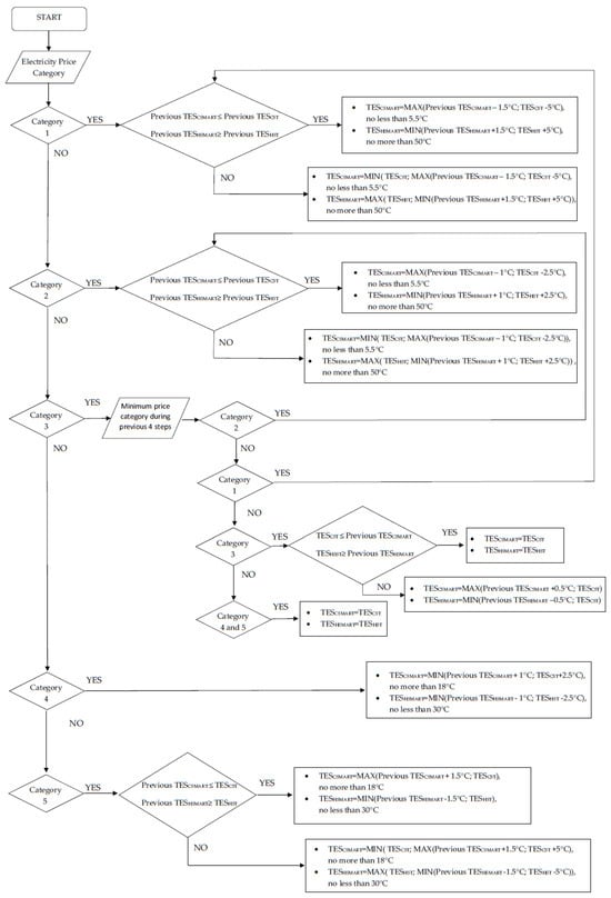
Figure 3.
Smart control strategy (price only) algorithm.
In addition to adjustments to the TES tanks’ temperatures, the algorithm also changes the DHW tank’s temperatures. The compensation values for each price category are presented in Table 3.
Table 3.
Smart control temperature compensation for DHW.
2.3.3. Smart Control Strategy (Price and PV)
Energy consumption from simulations of hydronic systems with the price only strategy was added to the remaining circuits measured in the CSIRO study for each timestep. It created the electric demand profile of the entire household. Then, PV generation was deducted from this load, creating an electricity import and export profile. If the balance was negative (electricity export), tank temperatures were again adjusted. It was conducted only for timesteps with categories 1 and 2 according to the equations below:
where Ee is electricity export from the household, COPav is the annual average COP for the task from the smart strategy (price only) simulations, Cp is the specific heat of water (0.00116 kWh/(kg·K)), and V is a volume of the tank. This forces the heat pump to work during periods of overgeneration using surplus energy and charging tanks. Because this algorithm affects the timesteps with price categories 1 and 2, the excessive load is only consumed when the grid already suffers from overgeneration. Other categories are not subjected to the algorithm. Therefore, the household would still contribute to the grid supply when it is beneficial. The adjusted smart control strategy (price and PV) sets were imported to the TRNSYS model, and simulations for the last scenario were conducted. Table 4 presents a short summary of all cases.
Table 4.
Summary of analysed scenarios.
3. Results
3.1. Total Energy Consumption and Average COP
The first analysed outcomes of the study are total energy consumption and average annual COP for each task and scenario. The simulation outcomes are presented in Table 5.
Table 5.
Annual total energy consumption and COP for each task and scenario.
All hydronic heating scenarios turned out to be much more efficient than conventional systems, reaching at least a 31.7% annual energy consumption reduction, mostly due to a higher COP for DHW preparation of heat pump systems. The GSHP systems were the most efficient in cooling and heating among all of the analysed options, using 18.6% and 23.9% less energy than conventional air conditioning for these tasks while working with a standard control strategy. The ASHP system with standard control used slightly more energy for cooling than AC, however, reaching a higher COP. This means that the ASHP transferred more thermal energy than the conventional system. Whereas for heating, the ASHP was more energy-conservative and reached a significantly higher COP than AC. It was also the most efficient way of preparing the DHW.
Both smart control strategies increased the energy consumption of hydronic systems. The lower COP is a result of forcing the heat pump systems to work in less favourable conditions, raising the water temperature for heating tasks and a decrease in cooling. Other contributors to increased energy consumption are higher tank heat loss and the fact that additional thermal energy in TES tanks could not be utilised and was wasted.
Looking only at total annual energy consumption, it can be said that hydronic systems are a good replacement for conventional solutions; however, smart control makes these systems less efficient. Nevertheless, the smart control strategy was not designed to decrease energy usage but to control the time when it occurs.
3.2. Space Conditioning and DHW Load Distribution
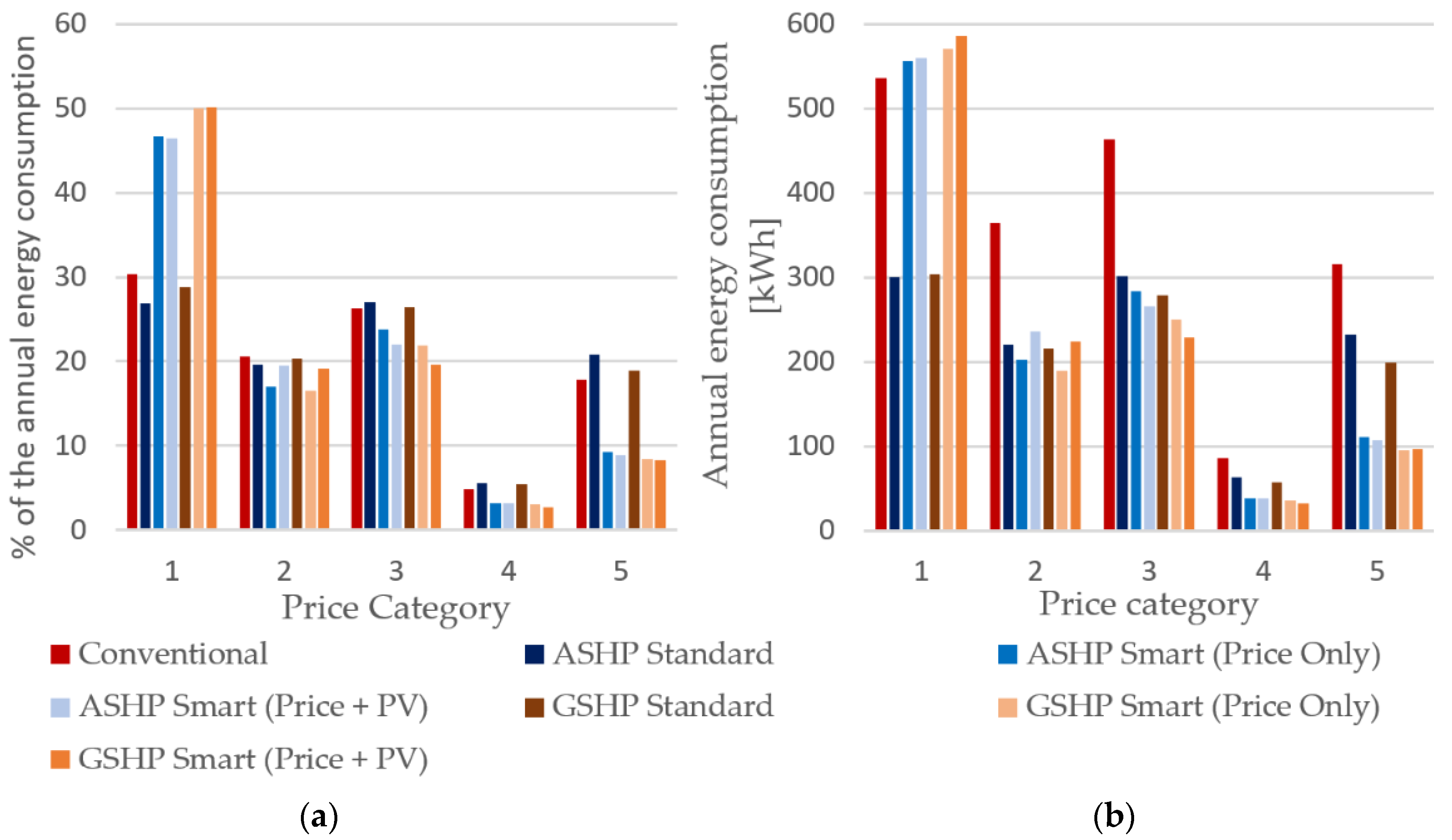
The energy consumption of the analysed systems was measured for each price category, and the results are presented in Figure 4.
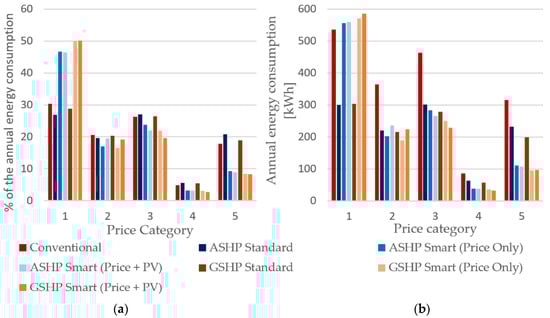
Figure 4.
Space conditioning and DHW heating energy consumption in each category: (a) percentage; (b) total.
There are no significant differences in the percentage load distribution for each price category of conventional and hydronic systems with standard control. However, hydronic systems with standard control systems used noticeably less energy in each price category than conventional AC and DHW heating. This means that hydronic systems can increase overall household efficiency. However, they do not bring any major help in stabilising the load. It is true that the system uses less energy during peak hours, but it also uses less energy during off-peak periods, making RES overgeneration even more problematic.
The smart control strategy caused hydronic systems to use around half of the electricity during price category 1 (ASHP 46–47%, GSHP 50%). The load distribution for the other categories dropped compared to conventional and hydronic standard systems. The largest decrease was noted in category 5. The electricity consumption in category 5 was halved compared to the standard control strategy and reduced by a third compared to the conventional system. The load in category 4 was also reduced. However, the change was not as radical. Categories 2 and 3 showed slightly less kWh usage using the smart strategy. Most of the load was shifted to category 1, where smart hydronic systems used even more energy than the conventional solution.
This means that even though a smart control strategy causes the hydronic system to use more energy, the consumption distribution is more favourable. The algorithm allowed the system to shift most of the load from categories 4 and 5 to category 1. Therefore, the household would contribute less to peak events and help utilise clean RES energy during periods of high generation.
3.3. Household Self-Consumption and Self-Sufficiency Levels
Another part of the analysis was to investigate the impact of hydronic systems on the utilisation of household-generated PV energy. For this purpose, self-consumption (SC) and self-sufficiency (SS) levels were calculated using Equations (6) and (7), where GT is total generation, CT is total consumption, ExpT is total export, and ImpT is total import. CT is the sum of AC, DHW, and the remaining loads. The results are presented in Table 6.
Table 6.
Household PV self-consumption and self-sufficiency levels.
Due to the fact that hydronic systems use less electricity than conventional systems, SC levels of PV generation for the standard and smart (price only) strategies decreased. However, the smart (price + PV) algorithm allowed for an increase in self-consumption to slightly over 81%, which is over one percentage point more than the result with the conventional system. So this solution not only helped reduce electricity consumption but also increased the utilisation of household-generated energy. This is confirmed by the highest self-sufficiency levels for both heat pumps with such a control system. Despite that, the system based on the GSHP reached a slightly lower level of SC than the ASHP; the overall balance in household self-sufficiency for this heat pump was the greatest among all of the analysed cases. This was caused by lower energy consumption and a higher COP of the system during overproduction periods. The highest PV generation usually occurs at the same time as the highest outdoor temperature. Therefore, the ASHP needs to work harder to transfer the heat to the sink with a higher temperature in a cooling-dominated climate. A ground heat exchanger provides a much more stable sink temperature.
3.4. Electricity Import and Export Distribution
The entire household’s electricity import and export loads were calculated and divided into price categories. These loads are the sum of AC, DHW, and the remaining loads minus PV generation. Table 7 presents these results.
Table 7.
Annual household electricity import (red, positive values) and export (green, negative values) for each price category.
Typical household electricity import for all hydronic heating cases and price categories 2–5 was lower than for the conventional system. The largest reduction in consumption was noted for category 5 for all four smart control strategies. The ASHP-based system helped to save 34.9–35.5%, while the GSHP-based system reduced the load by 37.4–37.6% during the highest peak events. Electricity import for the standard control strategy in category 1 dropped compared to the conventional solution; however, the smart control strategy allowed for reaching similar or slightly higher values. This confirms the earlier conclusions that smart hydronic systems are able to shift the load from peak to off-peak periods. Households with such systems would strain the grid much less than those with conventional air conditioning and water heating.
In addition to the electricity import, the smart (price + PV) control allowed for the decrease in electricity exports for categories 1 and 2, which was desirable in overgeneration limitation. Unfortunately, not all of the absorbed surplus energy was efficiently used. The ASHP smart (price + PV) system reduced exports by 60 kWh, but it saved only 45 kWh on electricity imports compared with ASHP smart (price only). The numbers for GSHP smart (price + PV) were even less optimistic, as the system reduced exports by 64 kWh and imports by 37 kWh. The most likely cause was the lower COP of the heat pumps that worked with extended temperature sets, as well as the fact that stored thermal energy was not utilised in time.
3.5. Space Conditioning and DHW Heating Fulfilment
As discussed earlier, one of the benefits of hydronic systems is that they can store energy in a TES tank instead of habitable space and use the reserves when the electricity load of heating and cooling devices needs to be limited. While earlier subsections showed improvements in energy consumption and distribution, Table 8 presents how smart strategies impacted the level of space conditioning fulfilment. The heating and cooling load has been considered to be fulfilled if the fan coil unit used to establish heating and cooling curves (Section 2.3.1) can cover the current space conditioning load with the current water temperature in the system.
Table 8.
Hydronic heating and cooling load fulfilment.
Results for standard control strategies showed very minimal under-conditioning in both time and loads. Undoubtedly, the TRNSYS simulations’ accuracy could be a major part of these numbers. Therefore, they can be treated as the basis for comparison with smart strategy cases.
Smart strategies lowered the level of satisfaction, but the decrease was not substantial. All systems still provided the required heating and cooling for over 99% of the time in the year. They also provided around 98.5% of the cooling load and 99.3–99.5% of the heating load. This means that the major amount of shifted electrical load barely affected indoor comfort. This achievement would not be possible for conventional air conditioning.
Overheating and over-cooling are not a problem due to the fact that space conditioning circuits are controlled independently. Therefore, even if the water temperature is higher than required for heating or lower than needed for cooling, the output can be adjusted to match the demand by various methods such as an on/off controller, variable speed pump, or variable airflow of a fan coil unit.
Also, DHW preparation was checked against the drop in the satisfactory level. The results, which are presented in Table 9, show that the temperature of the DHW outlet dropped below the recommended level of 50 °C in only marginal periods.
Table 9.
Percent of time with DHW temperature below 50 °C.
4. Study Discussion and Limitations
The presented research was focused on the estimation of the impact of replacement of a conventional cooling and heating system with a hydronic heat pump system with smart management on the electrical load generated by a typical South Australian household in the context of the transition towards net zero emissions.
In contrast to most of the research studies regarding the utilisation of hydronic heat pumps to stabilise the grid, it was decided to use measured electricity and hot water usage data. This allowed for the consideration of factors such as behavioural patterns and usage preferences, not only simulated cooling and heating loads. The peak load phenomenon is largely caused by the residential sector, especially AC. Therefore, it is crucial to include the household residents’ factors in the analysis. Also, measured data allows for the accurate use of other inputs, such as electricity price and weather conditions, which are aligned and represent the same events. However, the usage of measured AC electricity consumption required the calculation of cooling and heating loads. This process required some assumptions and simplifications. This process could cause some distortion of the simulations’ input data and results. Moreover, it has to be remembered that the typical household is only a theoretical concept. Most likely, none of the households participating in the CSIRO study had electricity use similar to the typical one. Therefore, extreme events can be distorted due to the results from multiple houses being averaged. Nevertheless, the considered solution aims to help not only households but mostly the national grid and its stability to allow further transition towards net zero emissions, which justifies this approach.
The peak cooling and heating loads, as well as the total energy consumption for space conditioning, may seem relatively low. As mentioned above, the distortion in peak loads could be one of the contributors. Moreover, typically in Australia, only the most used rooms are equipped with air conditioning. The low inertia of the AC system also means that they tend to be turned on and off as needed. However, hydronic systems work with much larger inertia, especially systems such as underfloor heating or cooling. Therefore, they usually maintain the temperature of the space at a relatively steady level for a longer period of time. Also, a hydronic heating plant room is a relatively large investment cost compared to an AC system. Therefore, it is usually more profitable to install a distribution system in the entire habitable space of the house. This could increase heating and cooling loads, also affecting energy consumption. These factors have not been taken into account in this project.
The smart control strategies used in this study were designed for this project. The parameters were adjusted multiple times until the results of the simulations were considered satisfactory. Too conservative an approach had too little influence on the base load profile to be considered meaningful. In turn, too aggressive values highly impacted load fulfilment levels, which could cause a decrease in the satisfaction level of users of such a system. One of the main advantages of hydronic heat pump systems over conventional AC is the ability to store energy and provide only the required cooling or heating load. Therefore, the balance between the grid needs and users’ comfort needs to be carefully considered. It is possible that the smart strategies could be even better tuned. However, this was not the main scope of the study. Also, the use of proprietary control strategies can be considered a limitation of the results of this study. However, similar systems have already been developed, and they are in use. An example of such a system is the smart grid ready (SG Ready) protocol introduced in Germany. However, it has become a standard heat pump feature in devices manufactured by world-leading companies. The protocol allows for external control of heat pumps by two zero-voltage contacts [41]. The contact can trigger four heat pump states: blocked operation, normal operation, encouraged operation, and forced operation. Therefore, the principle of operation is similar to the system analysed in this study. The heat pump market in Australia is still small. If smart heat pump systems are implemented in Australia, it could be the already developed SG Ready protocol or a new program suited to the local needs. The program could include model predictive control (MPC), which was not accounted for in this study. The MPC could help in the accurate preparation of TES and DHW tanks before the anticipated peak event and prevent unnecessary energy losses if the peak is not predicted and the surplus RES energy can be utilised elsewhere.
5. Conclusions
The analysis of the effects of replacing a conventional system consisting of an air conditioning unit and electric water heater with a hydronic heat pump system with smart control in a typical South Australian household presented in this paper provides promising results in shifting residential electrical load. All of the analysed scenarios bring some benefits to the load generated by the household. Hydronic systems with standard control drastically decreased energy consumption, mostly due to providing much more efficient DHW preparation. Smart control with the price only algorithm helped to significantly reduce electricity consumption during the periods of the highest electricity price, which appears when there is insufficient generation. Most of this load is shifted to the periods with the lowest electricity price, indicating too much supply. A system based on a ground source heat pump controlled by this control strategy used half of the total annual electricity consumption during price category 1. A further version of the smart control system, which added a module reacting to excessive PV generation, allowed for self-consumption and self-sufficiency levels. It also limited the export of the surplus load during periods of overgeneration. The difference in performance between systems based on an ASHP and a GSHP was slight. The GSHP achieved marginally less consumption and was able to shift more load. Thanks to the storage ability of water in TES tanks, the actions focused on adjusting the heat pump output barely impacted the space conditioning load. The load was satisfied for over 99.1% of the time. Only about 1.5% of the cooling load and 0.5–0.7% of the heating load were not delivered. Compared to the amount of shifted electricity, these numbers are rather insignificant. Nevertheless, they could be improved by tuning the cooling and heating curves, adjusting the algorithm values, or upsizing the FCU to allow for more capacity during the periods when the system relies on stored energy.
Therefore, it can be concluded that a hydronic system with a heat pump and smart control in a typical South Australian household can be a great tool in managing residential load. The problem with grid stability intensifies. Each year, Australia increases the capacity of domestic PV systems and the number of small AC units. Along with other grid stability problems, the Australian electricity network faces a huge challenge in the coming years. Efforts related to the Australian plan of reaching net zero emissions in 2050 could be squandered if the power network fails. The analysis presented in this paper was conducted using data measured in 2016. Currently, the price fluctuations are larger. This could make the aforementioned solutions even more beneficial.
Author Contributions
Conceptualization, A.R. and R.N.; Methodology, A.R. and R.N.; Software, A.R. and R.N.; Validation, A.R. and R.N.; Formal analysis, A.R., R.N. and M.J.; Investigation, A.R. and R.N.; Resources, R.N.; Data curation, A.R. and R.N.; Writing—original draft, A.R.; Writing—review & editing, R.N. and M.J.; Visualization, A.R. and R.N.; Supervision, R.N. and M.J.; Project administration, R.N. and M.J.; Funding acquisition, R.N. All authors have read and agreed to the published version of the manuscript.
Funding
This research received no external funding.
Data Availability Statement
The original contributions presented in the study are included in the article, further inquiries can be directed to the corresponding authors.
Conflicts of Interest
The authors declare no conflict of interest.
References
- Australian Government. Australia’s Long-Term Emissions Reduction Plan. A Whole-of-Economy Plan to Achieve Net Zero Emissions by 2050; Australian Government Department of Industry, Science, Energy and Resources: Canberra, Australia, 2021.
- Australian Government—Department of Climate Change, Energy, the Environment and Water. Residential Buildings. Available online: https://www.dcceew.gov.au/energy/energy-efficiency/buildings/residential-buildings (accessed on 20 April 2024).
- Boretti, A. Energy storage needs for an Australian national electricity market grid without combustion fuels. Energy Storage 2019, 2, e92. [Google Scholar] [CrossRef]
- Bayborodina, E.; Negnevitsky, M.; Franklin, E.; Washusen, A. Grid-Scale Battery Energy Storage Operation in Australian Electricity Spot and Contingency Reserve Markets. Energies 2021, 14, 8069. [Google Scholar] [CrossRef]
- ENERGEIA. Trajectory for Low Energy Buildings: Infrastructure and Customer Impacts; Prepared for Department of Environment and Energy: Sydney, Australia, 2019. [Google Scholar]
- Arraño-Vargas, F.; Shen, Z.; Jiang, S.; Fletcher, J.; Konstantinou, G. Challenges and Mitigation Measures in Power Systems with High Share of Renewables—The Australian Experience. Energies 2022, 15, 429. [Google Scholar] [CrossRef]
- Fan, H.; MacGill, I.F.; Sproul, A.B. Statistical analysis of drivers of residential peak electricity demand. Energy Build. 2017, 141, 205–217. [Google Scholar] [CrossRef]
- Australian PV Institute. Available online: https://pv-map.apvi.org.au/historical (accessed on 6 April 2024).
- Brodribb, P.; McCann, M.; Franjić, J.; Dewerson, G. Heat Pumps—Emerging Trends in the Australian Market; Expert Group for Australian Government: Brighton, VIC, Australia, 2023.
- Climate Council of Australia. Submission to the Senate Economics References Committee Inquiry into Residential Electrification. Available online: https://www.climatecouncil.org.au/wp-content/uploads/2023/10/Residential-Electrification-Submission.docx.pdf (accessed on 7 April 2024).
- Narayanan, R.; Sethuvenkatraman, S.; Pippia, R. Energy and Comfort Evaluation of Fresh Air-Based Hybrid Cooling System in Hot and Humid Climates. Energies 2022, 15, 7537. [Google Scholar] [CrossRef]
- Hashmi, S.A.; Ali, C.F.; Zafar, S. Internet of things and cloud computing-based energy management system for demand side management in smart grid. Int. J. Energy Res. 2020, 45, 1007–1022. [Google Scholar] [CrossRef]
- Mahapatra, C.; Moharana, A.K.; Leung, V.C.M. Energy Management in Smart Cities Based on Internet of Things: Peak Demand Reduction and Energy Savings. Sensors 2017, 17, 2812. [Google Scholar] [CrossRef] [PubMed]
- Hossein Motlagh, N.; Mohammadrezaei, M.; Hunt, J.; Zakeri, B. Internet of Things (IoT) and the Energy Sector. Energies 2020, 13, 494. [Google Scholar] [CrossRef]
- Ono, T.; Hagishima, A.; Tanimoto, J. Evaluation of potential for peak demand reduction of residential buildings by household appliances with demand response. Electron. Commun. Jpn. 2022, 105, e12379. [Google Scholar] [CrossRef]
- Energy Made Easy. Available online: https://www.energymadeeasy.gov.au/hot-topics/understanding-controlled-loads (accessed on 6 April 2024).
- Energex-PeakSmart Air Conditioning. Available online: https://www.energex.com.au/manage-your-energy/cashback-rewards-program/peaksmart-air-conditioning (accessed on 6 April 2024).
- Ember Pulse. Available online: https://emberpulse.com/ (accessed on 6 April 2024).
- Smith, R.; Meng, K.; Dong, Z.; Simpson, R. Demand response: A strategy to address residential air-conditioning peak load in Australia. J. Mod. Power Syst. Clean Energy 2013, 1, 223–230. [Google Scholar] [CrossRef]
- Tongsopit, S.; Junlakarn, S.; Wibulpolprasert, W.; Chaianong, A.; Kokchang, P.; Hoang, N.V. The economics of solar PV self-consumption in Thailand. Renew. Energy 2019, 138, 395–408. [Google Scholar] [CrossRef]
- Yu, H.J.J. System contributions of residential battery systems: New perspectives on PV self-consumption. Energy Econ. 2021, 96, 105151. [Google Scholar] [CrossRef]
- Fina, B.; Roberts, M.B.; Auer, H.; Bruce, A.; MacGill, I. Exogenous influences on deployment and profitability of photovoltaics for self-consumption in multi-apartment buildings in Australia and Austria. Appl. Energy 2021, 283, 116309. [Google Scholar] [CrossRef]
- Kamboj, S.; Narayanan, R. Ground Heat Exchangers for Cooling and Heating Applications in Buildings. In Reference Module in Earth Systems and Environmental Sciences; Elsevier: Amsterdam, The Netherlands, 2023. [Google Scholar]
- Fischer, D.; Madani, H. On heat pumps in smart grids: A review. Renew. Sustain. Energy Rev. 2017, 70, 342–357. [Google Scholar] [CrossRef]
- Péan, T. Heat Pump Controls to Exploit the Energy Flexibility of Building Thermal Loads; Universitat Politècnica de Catalunya: Barcelona, Spain, 2021. [Google Scholar]
- Dallmer-Zerbe, K.; Fischer, D.; Biener, W.; Wille-Haussmann, B.; Wittwer, C. Droop controlled operation of heat pumps on clustered distribution grids with high PV penetration. In Proceedings of the 2016 IEEE International Energy Conference (ENERGYCON), Leuven, Belgium, 4–8 April 2016; pp. 1–6. [Google Scholar]
- Kok, K.; Roossien, B.; MacDougall, P.; van Pruissen, O.; Venekamp, G.; Kamphuis, R.; Laarakkers, J.; Warmer, C. Dynamic pricing by scalable energy management systems - Field experiences and simulation results using PowerMatcher. In Proceedings of the 2012 IEEE Power and Energy Society General Meeting, San Diego, CA, USA, 22–26 July 2012; pp. 1–8. [Google Scholar]
- Vorushylo, I.; Keatley, P.; Shah, N.; Green, R.; Hewitt, N. How heat pumps and thermal energy storage can be used to manage wind power: A study of Ireland. Energy 2018, 157, 539–549. [Google Scholar] [CrossRef]
- Li, Y.; Mojiri, A.; Rosengarten, G.; Stanley, C. Residential demand-side management using integrated solar-powered heat pump and thermal storage. Energy Build. 2021, 250, 111234. [Google Scholar] [CrossRef]
- Li, Y.; Rosengarten, G.; Mojiri, A. Performance sensitivity of hot and cold thermal storage with onsite photovoltaics and heat pumps. Solar Energy 2023, 263, 111946. [Google Scholar] [CrossRef]
- CSIRO. Typical House Energy Use. Available online: https://ahd.csiro.au/other-data/typical-house-energy-use/ (accessed on 7 April 2024).
- Rapucha, A.; Narayanan, R.; Jha, M. Impact of Smart Hydronic System with Heat Pump on Electricity Load of a Typical Queensland Household. In Future Energy; Green Energy and Technology; Springer: Cham, Switzerland, 2023; pp. 163–172. [Google Scholar]
- Mitsubishi Electric MSZ-AP DataBook. Available online: https://www.mitsubishi-les.info/database/servicemanual/files/DataBook_2018_M_Pseries.pdf (accessed on 17 September 2022).
- Meteostat. Adelaide Weather Data. Available online: https://meteostat.net/en/station/94672?t=2016-01-01/2016-12-31 (accessed on 7 April 2024).
- Commonwealth of Australia. Water Heating Data Collection and Analysis, Residential End Use Monitoring Program (REMP); Commonwealth of Australia: Canberra, Australia, 2012. [Google Scholar]
- Ecoforest Geothermia. Technical Data Sheets-Ecoforest Heat Pumps. Available online: https://www.ecoforest.com/wp-content/uploads/2022/01/DS_Ecoforest_heat_pumps_EN_v2021_02_LQ.pdf (accessed on 7 April 2024).
- Mitsubishi Electric Air to Water Heat Pump Systems-Data Book Vol.4. Available online: https://www.mitsubishi-les.info/database/servicemanual/files/201803_ATW_DATABOOK.pdf (accessed on 7 April 2024).
- Fischer, D.; Lindberg, K.B.; Madani, H.; Wittwer, C. Impact of PV and variable prices on optimal system sizing for heat pumps and thermal storage. Energy Build. 2016, 128, 723–733. [Google Scholar] [CrossRef]
- AEMO. Aggregated Price and Demand Data. Available online: https://aemo.com.au/energy-systems/electricity/national-electricity-market-nem/data-nem/aggregated-data (accessed on 8 April 2024).
- Le, K.X.; Huang, M.J.; Wilson, C.; Shah, N.N.; Hewitt, N.J. Tariff-based load shifting for domestic cascade heat pump with enhanced system energy efficiency and reduced wind power curtailment. Appl. Energy 2020, 257, 113976. [Google Scholar] [CrossRef]
- Fischer, D.; Wolf, T.; Triebel, M.A. Flexibility of heat pump pools: The use of SG-Ready from an aggregator’s perspective. In Proceedings of the 12th IEA Heat Pump Conference 2017, Rotterdam, The Netherlands, 15–18 May 2017. [Google Scholar]
Disclaimer/Publisher’s Note: The statements, opinions and data contained in all publications are solely those of the individual author(s) and contributor(s) and not of MDPI and/or the editor(s). MDPI and/or the editor(s) disclaim responsibility for any injury to people or property resulting from any ideas, methods, instructions or products referred to in the content. |
© 2024 by the authors. Licensee MDPI, Basel, Switzerland. This article is an open access article distributed under the terms and conditions of the Creative Commons Attribution (CC BY) license (https://creativecommons.org/licenses/by/4.0/).