PEMFC Electrochemical Degradation Analysis of a Fuel Cell Range-Extender (FCREx) Heavy Goods Vehicle after a Break-In Period

Abstract

With the increasing focus on decarbonisation of the transport sector, it is imperative to consider routes to electrify vehicles beyond those achievable using lithium-ion battery technology. These include heavy goods vehicles and aerospace applications that require propulsion systems that can provide gravimetric energy densities, which are more likely to be delivered by fuel cell systems. While the discussion of light-duty vehicles is abundant in the literature, heavy goods vehicles are under-represented. This paper presents an overview of the electrochemical degradation of a proton exchange membrane fuel cell integrated into a simulated Class 8 heavy goods range-extender fuel cell hybrid electric vehicle operating in urban driving conditions. Electrochemical degradation data such as polarisation curves, cyclic voltammetry values, linear sweep voltammetry values, and electrochemical impedance spectroscopy values were collected and analysed to understand the expected degradation modes in this application. In this application, the proton exchange membrane fuel cell stack power was designed to remain constant to fulfil the mission requirements, with dynamic and peak power demands managed by lithium-ion batteries, which were incorporated into the hybridised powertrain. A single fuel cell or battery cell can either be operated at maximum or nominal power demand, allowing four operational scenarios: maximum fuel cell maximum battery, maximum fuel cell nominal battery, nominal fuel cell maximum battery, and nominal fuel cell nominal battery. Operating scenarios with maximum fuel cell operating power experienced more severe degradation after endurance testing than nominal operating power. A comparison of electrochemical degradation between these operating scenarios was analysed and discussed. By exploring the degradation effects in proton exchange membrane fuel cells, this paper offers insights that will be useful in improving the long-term performance and durability of proton exchange membrane fuel cells in heavy-duty vehicle applications and the design of hybridised powertrains.

1. Introduction

With the urgent need to mitigate greenhouse gas emissions and combat climate change, the automotive industry is rapidly shifting towards cleaner and more sustainable transportation solutions. One such innovation is the Fuel Cell Hybrid Electric Vehicle (FCHEV), which is capable of achieving net-zero emissions in the transportation sector. FCHEVs offer a compelling alternative to conventional internal combustion engines, delivering higher energy efficiency and zero harmful emissions.

As FCHEVs gain traction in research and development (R&D), it is important to ensure their long-term performance and durability. This study aims to understand the degradation mechanisms of proton exchange membrane fuel cells (PEMFCs) in Class 8 (gross vehicle mass > 15,000 kg) fuel cell range-extender (FCREx) hybrid heavy goods vehicles (HGVs) during their initial break-in period. The break-in or mechanical run-in period typically refers to the first 300 to 1600 km of a new vehicle, suggested by Clifford from Toyota [1]. During this period, high-speed or frequent motorway driving is not recommended [1]. An FCREx consists of a medium power PEMFC stack and a moderate capacity battery, as opposed to a high powered PEMFC stack and small capacity battery in a conventional parallel FCHEV [2]; a study by Molina et al. found that the overall H₂ and energy consumption can increase by 6.8% and 25%, respectively, when comparing an FCREx to a parallel FCHEV powertrain [3]. In an FCREx vehicle, the goal of the PEMFC stack is to achieve base driving, while the batteries account for dynamic and peak power demands. FCRExs are a promising configuration to support the trucking industry, where quick refuelling times and long driving ranges are key design factors. Commercially available options, such as the Tevva 7.5 tonne Hydrogen Electric Truck, are already under development [4].

PEMFCs are prone to experience degradation from pollution and fuel starvation [5]; and severe fuel starvation may introduce cell reversal [6]. A major benefit of the FCREx configuration is the prolonged durability. Meng et al. conducted a study on the degradation effects of dynamic current cycles of PEMFCs in vehicular applications; fuel starvation and lag were considered to be the main cause of irreversible degradation [7]. In Meng’s study, the PEMFC follows a more dynamic profile than the range-extender vehicle configuration in this study. Chandran et al. conducted a similar study on dynamic current loads, and suggested that load change, with a contribution percentage of 56.78%, and frequent start–stop, with a contribution percentage of 33.17%, is the main cause of PEMFC degradation in an automotive scenario [5]. While an FCHEV range-extender setup may encounter less load changes than a parallel PEMFC setup, there may be instances where the PEMFC has to be shut-off to prevent overcharging the battery, which may introduce frequent start–stop. Desantes et al. conducted a study to improve the durability of FCREx PEMFCs by imposing restrictions on power loads and transientness; it was found that the most evident cause of degradation was related to load changes [2].

Scaled-down bench testing offers a controlled environment to simulate operating conditions and accelerate degradation processes, replicating the real-life driving dynamics of FCHEVs in a laboratory setting. A key aspect of the project involves the development of drive-cycle-based bench testing tailored to range-extender FCHEV operation, enabling characterisation of power division [8]. Power cycles can be computed from drive cycles to estimate the power consumption of a vehicle as whole. These power cycles can then be divided into two or more separate drive cycles to simulate power division in a hybrid vehicle [8]. These divided power cycles can be scaled down to a cell level to facilitate cell bench testing in an electrochemical lab [8].

The degradation characterisation used in this study focuses on electrochemistry techniques, such as polarisation curves, cyclic voltammetry (CV), linear sweep voltammetry (LSV), and electrochemical impedance spectroscopy (EIS), to characterise degradation. These techniques provide invaluable insights into the electrochemical performance of PEMFCs. When considered alongside vehicle parameters, power cycle calculation, division, and downscaling, PEMFC preparation, testing, and operational parameters, and EIS equivalent circuits that fit the results are compared on a case-by-case scenario of a range of potential design scenarios.

2. Methodology

Figure 1 presents the procedural framework followed in this experiment. Both PEMFCs and LiBs were subjected to rigorous testing under conditions mirroring real-world driving scenarios. To replicate authentic electrochemical device testing in a vehicular context, part of the WHVC drive cycle was used to represent urban driving. These drive cycles were converted into power cycles, delineating the requisite power vs. time profiles for the Class 8 HGV.

These power requirements were pivotal in determining the optimal sizing of the energy systems encompassing fuel cells and batteries for the respective electrochemical hybrid vehicles. The division of power cycles between two primary electrochemical sources, namely proton exchange membrane fuel cell (PEMFC) stacks and lithium-ion battery (LiB) packs, was executed using a simple energy management strategy which estimates range-extender vehicles, where the PEMFC stack stays at a relatively constant average power while the LiB pack accounts for transient and peak power demands and was developed in Mathworks Matlab 2019a [9]. The Matlab programme, HybeMass V1.0, included electrochemical sources at either the pack level or stack level, specifically calibrated to provide the propulsive force requisite for an actual road vehicle [9]. To qualify for a Class 8 HGV, the gross vehicle mass (GVM) of the vehicle needs to exceed 15,000 kg. For the vehicle examples modelled in this study, the GVM ranges from 35,910 to 37,700 kg, depending on the cell operating powers used. The term ‘cell operating power’ refers to how much each individual cell will be stressed and will be discussed in detail in further sections. These GVM weights are similar to two soon-to-be commercially available net-zero Class 8 HGV, the electric battery Lion Electric 8T, which has a GVM of 37,200 kg [10], and the FCREx TransPower electric drayage truck, which has a GVM of 36,000 kg [11].

To enable appropriate degradation analysis, the power distribution across the electrochemical packs was downscaled to the cell level. The cells were then subjected to comprehensive testing and cycling using specialized Scribner 850E multi-range fuel cell testing stations and Biologic BCS-800 series battery cyclers. These experimental setups replicated the power demand that the fuel cell or battery would be subjected to in a vehicle, with variable load conditions demanded on a per-second basis.

2.1. Vehicle Dynamic Parameters

A Class 8 HGV (gross vehicle mass > 15,000 kg) was modelled using the HybeMass model [9]. The vehicle mass and dynamic parameters are presented in

Table 1. Vehicle mass and dynamic parameters of a Class 8 HGV scenario [9].

Parameters	Description	Value
Cd	Drag coefficient	0.36
A	Frontal area (m2)	9
GVM	Gross vehicle mass (kg)	37,195
$\rho$	Air density (kg m−1)	1.225
$c_{rr}$	Static rolling coefficient	0.008

. Parameters were selected and estimated based on existing literature and specification sheets [9,12]. The air density ($\rho$) value was the standard density at sea level and 15 °C. When running the model, a Matlab setup file was created before running the Simulink model to initialise the aforementioned parameters.

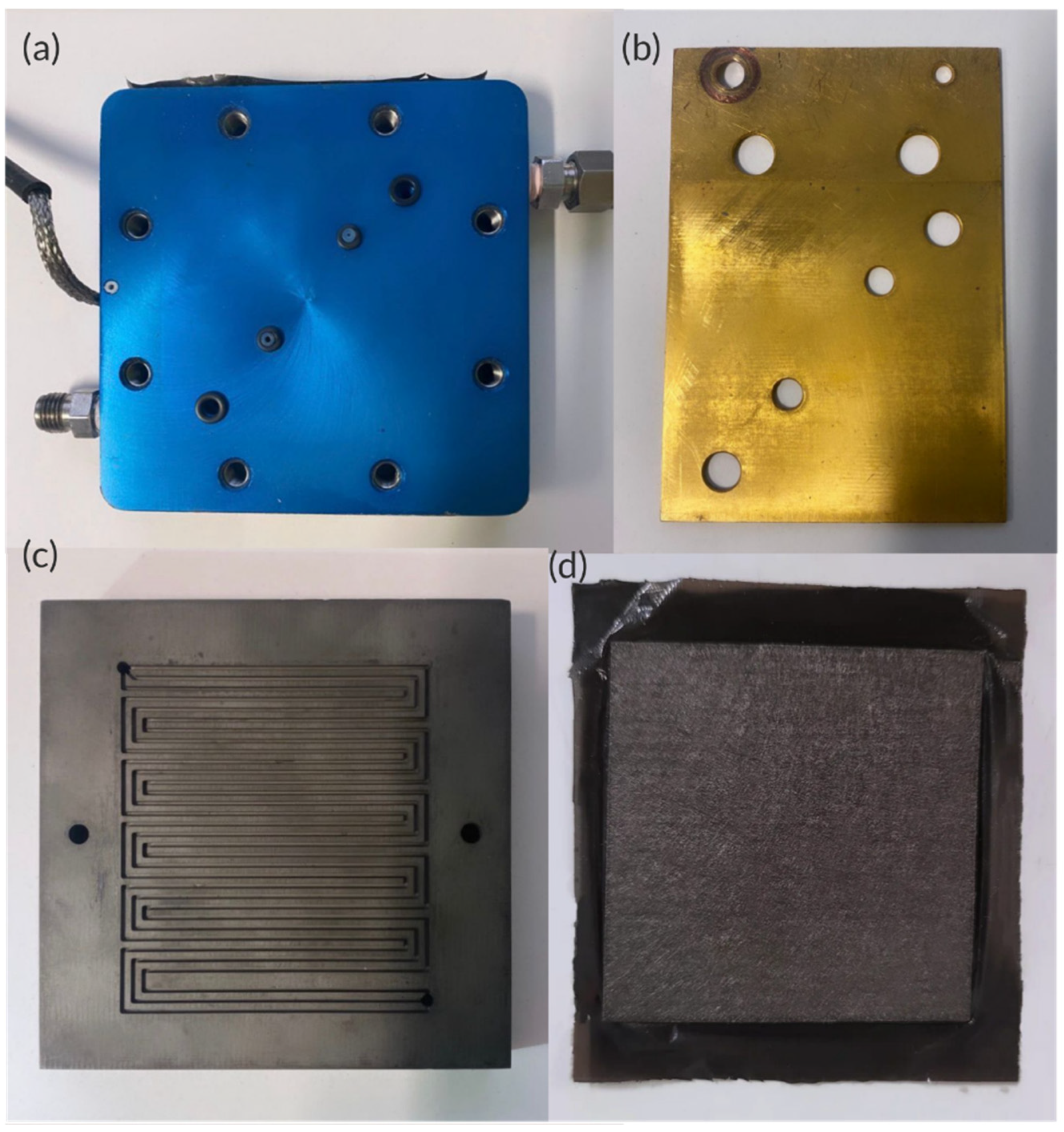
2.2. PEMFC Preparation, Specifications, and Operating Conditions

Scribner 850e was used to test a 25 cm² active area PEMFC, under various drive cycles. In addition, 100 continuous cycles of the WHVC drive cycle were tested; essentially, this analysis aimed to determine the severity of PEMFC degradation after 530 km of urban driving. As shown in Figure 2, the PEMFC used for testing consists of a polytetrafluoroethylene-based (PTFE) membrane, a carbon gas diffusion layer (GDL), a microporous layer (MPL) a platinum–carbon (Pt/C) catalyst, flow field plates and stainless-steel bipolar plates (BiPs). A PTFE-based membrane is usually referred to using its commercial names, such as Nafion or Gore-Select. The type used in the current study was Gore-Select, which was selected as it is widely used in the automotive sector, including in the Toyota Mirai FCHEV. Commercial carbon GDLs, MPLs and Pt/C catalysts were compressed using a hot press to form a gas diffusion electrode (GDE). The GDE used in this project was from the South African manufacturer HyPlat (0.4 mg_Pt cm⁻²) [13]. Flowfield plates and stainless BiPs, often referred to as end plates, were supplied by Scribner Associates.

Together, the GDL, Pt/C catalyst and PTFE membrane form the membrane electrode assembly (MEA) of the fuel cell. The membrane electrode assembly is assembled in-lab by ‘sandwiching’ the PTFE membrane between two HyPlat GDEs. A single HyPlat GDE has two sides, one consisting of the GDL and the other of the Pt/C catalyst. The two GDEs are oriented in such a way that the Pt/C sides face each other, with the PTFE membrane in between. A photograph of the layout is shown in Figure 2d. The MEA assembly was then hot-pressed for three minutes with a temperature of 150 °C on both the anode and cathode side, with a clamp force of 1700 lbs, or 7560 N. Then, the fuel cell was assembled in the order shown in Figure 2. The bolts used to hold together the fuel assembly were tightened with a final torque of 4 Nm.

The operating conditions of the PEMFC adhered to the EU Reference Automotive Conditions suggested by The Fuel Cells and Hydrogen Joint Undertaking (FCH JU). These conditions are listed in

Table 2. Scribner PEMFC operating parameters, following the FCH JU EU Reference Automotive Conditions [14].

Parameter	Unit	Value
Cell temperature	°C	80
Anode gas inlet dew point temperature (DPT)	°C	64
Anode gas inlet absolute pressure	kPa	250
Anode stoichiometry	-	1.3
Cathode gas inlet dew point temperature (DPT)	°C	53
Cathode gas inlet absolute pressure	kPa	230
Cathode stoichiometry	-	1.5

. The dew point temperatures (DPTs) for the anode and cathode were set at 64 °C and 53 °C, respectively, paired with a cell temperature of 80 °C, which allowed a relative humidity (RH) of 50% for the anode and 30% for the cathode [14]. Before any experiments, the fuel cell was conditioned by first heating the PEMFC to the desired operating temperature (80 °C) and holding it at that temperature for 30 min. The cell operated at a constant current of 5 A until the voltage stabilised. Later, polarisation curves from OCV to 0.3 V and 0.3 V back to OCV were collected until the curves were stable.

Figure 3 shows an example of a polarisation and power curve of a PEMFC fabricated in the lab. These cells typically reach a maximum power of 20 W or 0.8 W cm⁻², which would a key methodology design factor discussed in further sections. The power output was measured using a Scribner 850E multi-range fuel cell testing station. To ensure the quality of the MEAs manufactured in-lab, a BoL polarisation and power curve is usually collected before the start of any drive cycle endurance testing. The main three criteria were that OCV was more than 0.9 V, the current density at 0.3 V was more than 1600 mA cm⁻², and maximum power could reach 20 W. If these criteria were not met, the MEA was discarded. Because each MEA is hand-made, the performance may vary; it is important to focus on the delta polarisation performance decrease between the different configurations rather than the absolute.

Polarisation, CV, LSV, and EIS collection was conducted at BoL and EoT, with the operating conditions shown in

Table 3. Polarisation, CV, LSV, and EIS operation conditions.

Technique	Conditions
Polarisation curve	OCV to 0.3 V to OCV; 30 s pt−1; 0.025 V pt−1
CV	0.06 V to 1 V to 0.06 V; 20 mV/s; 0.1 s pt−1
LSV	0.06 V to 0.6 V; 5 mV s−1; 0.1 pt s−1
EIS	AC 10%; 10,000 to 0.1 Hz

.

2.3. Drive Cycle Endurance Testing for PEMFCs

Drive cycles are standardised driving data published in a speed vs. time format [8]. The dynamic load cycling endurance test was used to simulate 100 cycles of HGV urban driving, a distance of approximately 530 km, representing the break-in period of a vehicle. Typically, vehicle manufacturers do not recommend highway driving during this break-in period, so an urban-based drive cycle was the optimal choice for this analysis. The total distances of drive cycles were calculated by integrating the speed vs. time curves. The procedures for dynamic load testing took inspiration from FCH JU’s dynamic load cycling endurance test protocols. The FCH JU protocol was created for FCEVs (non-hybrids) and utilises the NEDC drive cycle [15]. However, the NEDC cycle is primarily a light-duty vehicle (LDV) modal drive cycle and is now considered outdated and less representative of realistic driving representation when compared to a WHVC and newer transient drive cycles [8]. Transient drive cycles are usually collected based on real-life driving data [8]. Figure 4 shows a comparison between WHVC Urban and the commonly used NEDC. As seen, WHVC Urban has a lower average speed that is more representative of HGV driving and is more transient and realistic than NEDC.

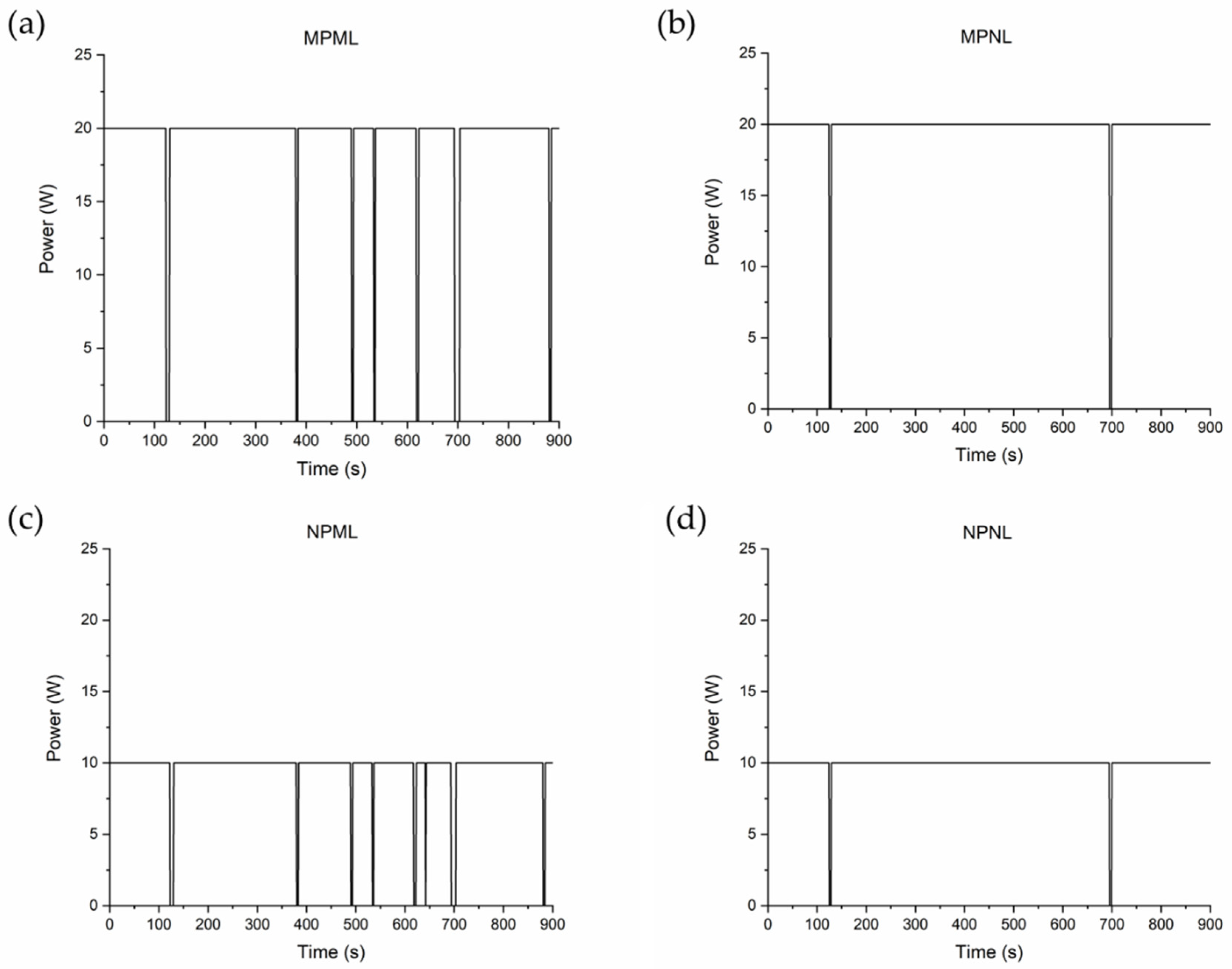
2.4. Power Cycle Division for a Range-Extender Vehicle

HGVs are typically designed for range as opposed to power due to the specific requirements of the vehicle as they lend themselves towards propulsion using PEMFCs, which is a well-known high gravimetric energy-density electrochemical system. An FCREx architecture is a valid solution to the utilisation of the energy-dense advantage of the PEMFC technology [9,15]. In this FCREx HGV, the PEMFC stack provides constant average power for $P_{req}$, while the LiB pack accounts for the remaining power. Keeping the PEMFC stack at a constant power is beneficial for prolonging the lifetime of the stack as PEMFCs do not cope well with transient demands [9]. Figure 5 shows an example of the required PEMFC stack, and LiB pack power profiles. It should be noted that while the PEMFC power is above the required power, the extra PEMFC stack can, and is, used to recharge the battery. It can also be seen that the PEMFC stack power does not stay perfectly constant; on occasion, the PEMFC stack power drops to 0 kW. This was a safety feature implemented to prevent the overcharging of LiBs from the PEMFC. During certain periods, the regenerative braking power alone is enough to provide maximum recharge power to the LiBs; any extra PEMFC power would not be utilised. It should be noted that the profiles may differ slightly depending on the PEMFC or the LiB’s cell operating power, which is a key design discussed in the next section.

2.5. Downscaling Stack-Level Power Cycles to Cell-Level Power Cycles

Using the HybeMass model [9], the required stack and pack-level power profiles could be extracted for both the PEMFC and battery components. These profiles were then scaled to a single cell level to be downscaled to a cell level to be tested on an electrochemical bench scale, in the units of W. The maximum stack or pack operational power of both the PEMFC stack and battery pack was computed. Then, a list of ratios relative to the maximum operational power ($r$) was compiled for the stack power of every timestamp (in seconds) of the drive cycle. The cell power of either the PEMFC or LiB cell at each time stamp ($P_i$) was calculated using the following equation:

$$P_i=P_{cell\_op}\times r_i$$

(1)

where $P_i$ is the required cell power at the $i$ timestamp of the drive cycle, $P_{cell\_op}$ is the cell operating power, and $r_i$ is the ratio of the required stack power at the $i$ timestamp to the maximum required stack power.

When downscaling stack-level power cycles to the cell level, cell operating power becomes a crucial design consideration. Both PEMFC and LiB cells can operate either at maximum power or nominal power to meet the vehicle’s power requirements. Bench testing of PEMFCs has shown a maximum power output of around 20 W or 0.8 W cm⁻², as illustrated in Figure 3, though this value can vary slightly depending on the quality of cells manufactured in-house. The nominal operating power is defined as half of the maximum power, which is 10 W or 0.4 W cm⁻² for the tested cell. While operating at nominal power increases the mass of the stack and pack, it is suggested that system durability improves as a result. Choosing the operating condition involves balancing factors such as cost, mass, and lifetime. To evaluate a range of considerations, four conditions were examined: maximum PEMFC power and maximum battery power (MPML), maximum PEMFC power and nominal battery power (MPNL), nominal PEMFC power and maximum battery power (NPML), and nominal PEMFC power and nominal battery power (NPNL), as detailed in

Table 4. Operational terminology and maximum power output of PEMFC and LiB cells.

Operation Terminology	PEMFC Maximum Power (W)	LiB Maximum Power (W)
MPML	20	20
MPNL	20	10
NPML	10	20
NPNL	10	10

. A typical PEMFC manufactured in-house by the experimenter would typically operate at a voltage of 0.65 to 0.70 V to obtain a power of 20 W, and a voltage of 0.75 to 0.80 V to obtain a power of 10 W.

Figure 6 outlines the cell power cycles for the PEMFC under the four different operating scenarios. As mentioned previously, the PEMFC has to shut off its power (0 W) during certain timestamps to prevent the LiB from overcharging. In scenarios with LiB cells operating at nominal power (suggesting a larger battery pack when compared to maximum cell operating power), there was less time in which the PEMFC had to be shut off.

2.6. ECSA Calculation

One of the main causes of PEMFC degradation caused by dynamic loads is the degradation of the Pt/C catalyst, particularly in the loss of ECSA [16]. The ECSA decay rate can be represented as a function of the remaining surface area of the Pt catalyst [16]. Figure 7 is an example of collected CV curves with labelled regions of interest. CV diagrams are shown for current (A), or current density (A cm⁻²) vs. voltage (V). ECSA estimation is calculated by integrating the curve of either the hydrogen atom desorption or adsorption region, as these two regions are proportional to the number of hydrogen molecules reactive with the Pt catalyst [17]. In this project, the adsorption region was always integrated instead of the desorption region to keep the data analysis consistent. The following equation was used to estimate ECSA [17]:

$$ECSA=\frac{Q_{Pt}}{\mathsf{\Gamma }L}$$

(2)

where $L$ is the mass of platinum per unit area (mg cm⁻²), which was 0.4 mg cm⁻² for HyPlat, $Q_{Pt}$ is the charge area of hydrogen adsorption or desorption, and $\mathsf{\Gamma }$ is the charge required to reduce a monolayer of protons on platinum (210 μC cm⁻²) in the unit of μC cm⁻².

ECSA estimations, however, can only capture degradation mechanisms within the activation and charge transfer regions, as it is mainly an estimation of catalyst availability. Nevertheless, it is still one of the most important characterisation techniques in this project as it provides valid numerical comparisons between all endurance testing scenarios.

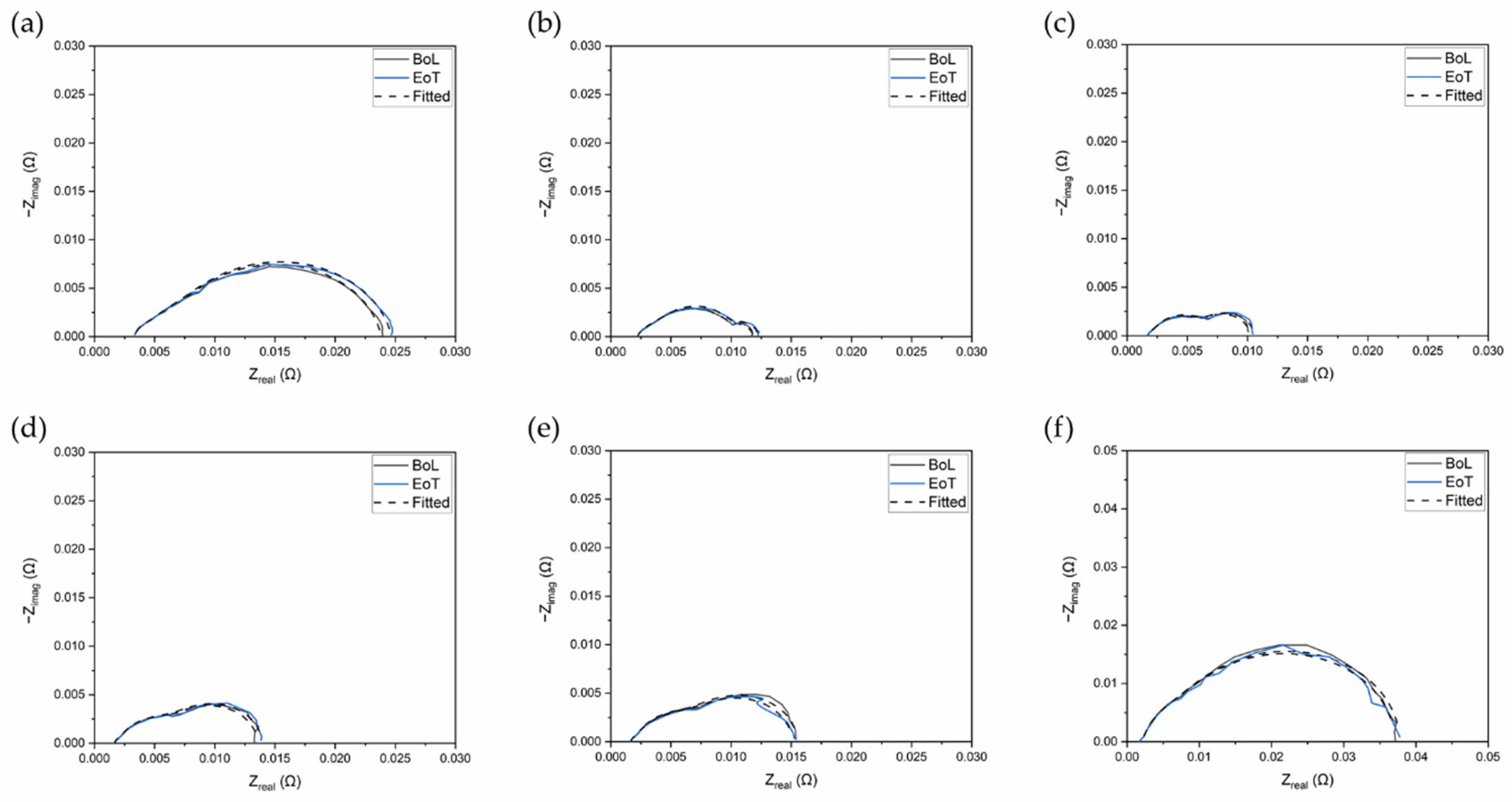
2.7. EIS Equivalent Circuit Model Fitting

EIS tests were conducted to compare the impedance between BoL and EoT. Nyquist plots were fitted into an equivalent circuit model using RelaxIS 3 3.0.22 Build 29 software. The equivalent circuit model used is shown in Figure 8. From this model, the Ohmic (R_Ω), anode charge transfer (R_an), cathode charge transfer (R_ca), and mass transfer (R_ca) resistance can be interpolated. A combination of constant phase elements (CPEs) and capacitors were used. A CPE is considered to be in between a resistor and a capacitor, which is arguably more representative and popularised for a PEMFC’s charge transfer region [18]. In addition, because CPEs have an extra degree of freedom than capacitors, the error of the fit is usually less [18,19]. One of the benefits of this model is that it differentiates between the anode and cathode charge transfer resistance separately, while keeping a low fitting error.

3. Results and Discussion

A general electrochemical degradation overview is presented in four subsections featuring the different cell operating power scenarios: MPML, MPNL, NPML, and NPNL. The last subsection provides a comparison between all scenarios, discussing the relative merits and demerits of the design choice for vehicles.

3.1. MPML

In theory, the MPML cell operating scenario has the capability of having the lightest power source configuration, allowing a reduced vehicle kerb, and gross vehicle mass (GVM); with the possible trade-off of more degradation of the power sources (each cell is stressed to the greatest extent). Figure 9 presents the electrochemical degradation analysis of the MPML cell operating power scenario. As shown in the polarisation and power curve in Figure 9a, at 600 mA cm⁻², the voltage decreased from 0.73 to 0.72 V between BoL and 100 WHVC cycles (EoT), suggesting a degradation rate of 1.37% or 0.055% h⁻¹. At 1200 mA cm⁻², the voltage decreased from 0.60 to 0.58 V between BoL and EoT, suggesting a degradation rate of 3.33% or 0.133% h⁻¹. Kurtz et al. at the US National Renewable Energy Laboratory (NREL) and Department of Energy (DOE) published similar data for an automotive-use PEMFC voltage degradation rate of 1200 mA cm⁻²; a value of 0.003% h⁻¹ was suggested [21]. By utilising the MPML configuration, the degradation rate at 1200 mA cm⁻² was higher than NREL and DOE lab tests. The maximum power dropped from 20 to 17 W, a 15% or 0.6% h⁻¹ decrease. This maximum power decrease suggests a major concern for this operating scenario, in that the PEMFC would no longer be capable of supporting the required allocated power demands (20 W or 0.8 W cm⁻² constant power) after the vehicle break-in period. In a real-life scenario looking to utilise a similar configuration to the MPML operating power, it is suggested that the PEMFCs are not stressed to the absolute maximum, but rather slightly below the maximum capable power, to account for this power decrease after the vehicle break-in period.

As shown in the cyclic voltammetry plot in Figure 9b, the ECSA decreased from 64.2 to 56.7 m² g⁻¹ between BoL and EoT, an 11.68% decrease. Figure 9c shows the LSV curve comparison between BoL and EoT. According to DOE standards, if the equilibrium part of the LSV exceeds a current density of 20 mA cm⁻², the cell is considered to be chemically unstable with severe hydrogen crossover [22], which is not the case for the EoT of this scenario. The hydrogen crossover rate changed from 1.17 × 10⁻⁶ to 1.36 × 10⁻⁶ mol s⁻¹ from BoL to EoT, a 16% increase.

Figure 10 shows Nyquist plots of both potentiostatic and galvonaostatic EIS collected at different current densities (100, 300, 800, and 1200 mA cm⁻²) and voltages (0.65 and 0.5 V) for the MPML scenario. Both the fitted and unfitted curves are plotted. For most current densities and voltages, the most significant change between BoL and EoT occurred at the low-frequency intercept with the real axis and the height of the semicircles. For the collection at 100 mA cm⁻², the largest changes occurred at the high-frequency intercept with the real axis and the height of the semicircles. The high-frequency intercept with the real axis infers the Ohmic resistance (R_Ω).

More information can be extracted by fitting the Nyquist plots with the equivalent circuit outlined in Figure 8. After fitting, different resistance values such as Ohmic resistance (R_Ω), anode (R_an) and cathode charge transfer resistance (R_ca), and mass transport resistance (R_m) can be interpolated, shown in

Table 5. Resistance values for the MPML scenario interpolated from EIS equivalent circuit fitting, including Ohmic resistance (R_Ω), anode (R_an) and cathode charge transfer resistance (R_ca), and mass transport resistance (R_m).

Current Density or Voltage (mA cm−2 or V)	RΩ BoL (mΩ cm2)	RΩ EoT (mΩ cm2)	Ran BoL (mΩ cm2)	Ran EoT (mΩ cm2)	Rca BoL (mΩ cm2)	Rca EoT (mΩ cm2)	Rm BoL (mΩ cm2)	Rm EoT (mΩ cm2)
100 mA cm−2	108	84.2	45.8	32.0	475	551	66.9	24.7
300 mA cm−2	72.6	64.5	77.4	79.2	74.4	94.8	123	148
800 mA cm−2	53.6	50.7	120	15.3	116	147	18.3	159
1200 mA cm−2	51.4	49.1	137	19.2	241	176	17.9	440
0.65 V	51.5	49.6	136	14.6	195	152	16.5	229
0.5 V	51.7	49.0	156	206	693	855	19.4	16.8

. Aside from the collection at 100 mA cm⁻², which is within the Ohmic region, all other instances of Ohmic resistance are negligible. In most current densities and voltages, the increase in cathode charge transfer resistance was the most dominant change between BoL to EoT, suggesting cathode degradation. For 1200 mA cm⁻², both anode and cathode charge transfer resistance decreased; however, there has been an increase in mass transport resistance. This corresponds with the polarisation curve results shown in Figure 9a, as the 1200 mA cm⁻² current density is within the charge transfer region at BoL but has shifted to the mass transport region at EoT, a non-favourable operating region for PEMFCs. An increase in mass transport may suggest a reduced water content of the membrane [21].

3.2. MPNL

With theory and assumption, the MPNL scenario would be the least advantageous configuration for an FCHEV. It is not recommended to operate a PEMFC at its maximum operating power unless a design goal is to minimise weight or allow for easier vehicle integration and packaging; while this is true for the PEMFC counterpart of the scenario, the nominal LiB (NL) design choice would almost double the amount of battery cells in a battery pack, increasing the overall mass of the powertrain. Figure 11 shows the electrochemical degradation analysis of the MPNL cell operating power scenario. As shown in the polarisation and power curve in Figure 11a, at 600 mA cm⁻², the voltage and power stayed at a consistent value of 0.75 V and 12 W between BoL and EoT. At 1200 mA cm⁻², the voltage stayed at a consistent value of 0.65 V between BoL and EoT. This degradation performance exceeds both NREL’s lab results and the 2020 DOE target of 0.002% h⁻¹ [21]. The maximum power dropped from 22 to 21 W, a 4.55% or 0.18% h⁻¹ decrease. Interestingly, judging solely from polarisation and power curves, the PEMFC had a 0% degradation rate at 600 mA cm² and 1200 mA cm². The PEMFC in this case had a more optimal degradation rate than the MPML scenario, where the PEMFC was also stressed to the maximum. A possible explanation is the more consistent power profile for the MPNL scenario, where the PEMFC experienced less shut-off time than the MPML scenario, allowing a less transient power profile.

As shown in the CV graph in Figure 11b, the ECSA decreased from 74.6 to 62.2 m² g⁻¹ between BoL and EoT, a 16.62% decrease. Figure 10c shows the LSV curve comparison between BoL and EoT. Based on the LSV measurements the cell is considered to be chemically stable at EoT according to DOE standards. Interestingly, the hydrogen crossover rate decreased from 8.42 × 10⁻⁷ to 8.16 × 10⁻⁷ mol s⁻¹, a 3% decrease.

Figure 12 shows Nyquist plots of both potentiostatic and galvonaostatic EIS collected at different current densities and voltages for the MPNL scenario. For all current densities and voltages, the most visual change between BoL and EoT occurred at the low-frequency intercept with the real axis and the height of the semicircles. In this scenario, the heights of the semicircles between BoL and EoT are similar except for the curve collected at 1200 mA cm², as a slight increase was seen along the imaginary axis.

The resistance values for the MPNL scenario were extracted and outlined in

Table 6. Resistance values for the MPNL scenario interpolated from EIS equivalent circuit fitting, including Ohmic resistance (R_Ω), anode (R_an) and cathode charge transfer resistance (R_ca), and mass transport resistance (R_m).

Current Density or Voltage (mA cm−2 or V)	RΩ BoL (mΩ cm2)	RΩ EoT (mΩ cm2)	Ran BoL (mΩ cm2)	Ran EoT (mΩ cm2)	Rca BoL (mΩ cm2)	Rca EoT (mΩ cm2)	Rm BoL (mΩ cm2)	Rm EoT (mΩ cm2)
100 mA cm−2	78.4	82.2	27.0	27.2	435	483	39.7	30.2
300 mA cm−2	60.0	63.9	170	186	46.2	50.7	23.0	24.0
800 mA cm−2	45.3	46.1	30.3	29.7	113	134	83.6	93.3
1200 mA cm−2	44.1	44.9	28.9	25.7	213	273	102	115
0.65 V	44.1	45.0	21.9	11.6	253	145	112	261
0.5 V	45.7	45.6	126	16.7	819	128	14.6	863

. The Ohmic resistance is small for all current densities and voltages. During all current densities and voltages, the increase in mass transport resistance was the greatest change between BoL to EoT, specifically for the potentiostaic EIS collections at 0.65 and 0.5 V. At 0.65 V during BoL, the PEMFC was still operating in a reasonable region within the polarisation curve, but at EoT, it was operating at the start of the mass transport region, a problematic region for PEMFCs. At 0.5 V, the PEMFC was operating at the end of the charge transfer region during BoL but has shifted to the problematic mass transport region at EoT; a severe increase in mass transfer resistance is shown in Table 6, which indicates a lowered water content of the cell to support the diffusion of oxygen [23].

3.3. NPML

The NPML scenario was assumed to be one of the most optimal setups for a range-extender FCHEV, where the PEMFC is not stressed to the maximum and the number of battery cells is kept to a minimum to reduce the weight of the heavier power system (battery pack). Figure 13 presents the electrochemical degradation analysis of the NPML cell operating power scenario. As shown in the polarisation and power curve in Figure 13a, at 600 mA cm⁻², the voltage decreased from 0.76 to 0.75 V between BoL and EoT, with a degradation rate of 1.32% or 0.053% h⁻¹. At 1200 mA cm⁻², the voltage decreased from 0.66 V to 0.65 V between BoL and EoT, with a degradation rate of 1.52% or 0.061% h⁻¹, which was higher than the NREL results and 2020 DOE standards [21]. The maximum power dropped from 24 to 23 W, a 4.17% or 0.17% h⁻¹ decrease.

As shown in the CV graph in Figure 13b, the ECSA decreased from 75.5 to 68.3 m² g⁻¹ between BoL and EoT, a 9.54% decrease. Figure 13c shows the LSV curve comparison between BoL and EoT. The cell is considered to be chemically stable at EoT according to DOE standards based on the LSV. The hydrogen crossover rate increased from 8.16 × 10⁻⁷ to 9.59 × 10⁻⁷ mol s⁻¹, an 18% increase.

Figure 14 shows Nyquist plots of both potentiostatic and galvonaostatic EIS collected at different current densities and voltages for the NPML scenario. For most current densities and voltages, the most visual change between BoL and EoT occurred at the low-frequency intercept with the real axis.

The resistance values for the NPML scenario were extracted and outlined in

Table 7. Resistance values for the NPML scenario interpolated from EIS equivalent circuit fitting, including Ohmic resistance (R_Ω), anode (R_an) and cathode charge transfer resistance (R_ca), and mass transport resistance (R_m).

Current Density or Voltage (mA cm−2 or V)	RΩ BoL (mΩ cm2)	RΩ EoT (mΩ cm2)	Ran BoL (mΩ cm2)	Ran EoT (mΩ cm2)	Rca BoL (mΩ cm2)	Rca EoT (mΩ cm2)	Rm BoL (mΩ cm2)	Rm EoT (mΩ cm2)
100 mA cm−2	84.0	83.8	52.7	32.6	89.8	455	350	45.1
300 mA cm−2	56.9	57.9	49.6	183	51.1	46.3	133	22.2
800 mA cm−2	44.2	44.4	108	20.9	91.8	107	10.1	90.2
1200 mA cm−2	43.5	43.8	120	113	168	176	8.80	10.7
0.65 V	42.3	43.8	26.2	116	224	193	96.8	10.9
0.5 V	45.1	45.4	18.1	15.2	769	121	129	705

. Mass transport resistance is negligible for all current densities and voltages. Anode and cathode charge transfer resistances were the main forms of impedance increase from BoL to EoT throughout most current densities and voltages. A severe mass transfer resistance was also spotted at 0.5 V, which can suggest a lowered water content of the cell [23].

3.4. NPNL

The NPNL scenario is a configuration that maximises the durability of both the PEMFC and LiB; it is also the heaviest option. Figure 15 presents the electrochemical degradation analysis of the NPNL cell operating power scenario. As shown in the polarisation and power curve in Figure 15a, at 600 mA cm⁻², the voltage stayed at a consistent value of 0.77 V between BoL and EoT. At 1200 mA cm⁻², the voltage decreased from 0.69 V to 0.68 V between BoL and EoT, suggesting a degradation rate of 1.45% or 0.058% h⁻¹, higher than NREL results and 2020 DOE standards [21]. The maximum power dropped from 25 to 24 W, a 4% or 0.16% h⁻¹ decrease.

As shown in the CV graph in Figure 15b, the ECSA decreased from 74.4 to 68.4 m² g⁻¹ between BoL and EoT, an 8.06% decrease. Figure 15c shows the LSV curve comparison between BoL and EoT. The cell is considered to be chemically stable at EoT according to DOE standards. The hydrogen crossover rate increased from 1.05 × 10⁻⁶ to 1.11 × 10⁻⁶ mol s⁻¹, a 5.7% increase.

Figure 16 shows Nyquist plots of both potentiostatic and galvonaostatic EIS collected at different current densities and voltages for the NPNL scenario. For the galvanostatic EIS collections, the most visual change between BoL and EoT occurred at the low-frequency intercept with the real axis. For the potentiostatic EIS collections, the height of the semicircles increased.

The resistance values for the NPNL scenario were extracted and outlined in

Table 8. Resistance values for the NPNL scenario interpolated from EIS equivalent circuit fitting, including Ohmic resistance (R_Ω), anode (R_an) and cathode charge transfer resistance (R_ca), and mass transport resistance (R_m).

Current Density or Voltage (mA cm−2 or V)	RΩ BoL (mΩ cm2)	RΩ EoT (mΩ cm2)	Ran BoL (mΩ cm2)	Ran EoT (mΩ cm2)	Rca BoL (mΩ cm2)	Rca EoT (mΩ cm2)	Rm BoL (mΩ cm2)	Rm EoT (mΩ cm2)
100 mA cm−2	85.0	84.3	31.5	32.9	425	450	54.6	49.7
300 mA cm−2	57.6	54.7	175	68.7	40.5	55.3	22.0	128
800 mA cm−2	43.4	43.0	110	112	91.8	97.9	9.80	10.6
1200 mA cm−2	42.5	42.1	125	123	163	173	8.90	9.40
0.65 V	42.5	41.7	124	141	209	187	12.0	8.20
0.5 V	43.9	43.8	153	166	732	703	14.2	12.4

. R_Ω is negligible for all current densities and voltages. Only minor resistances were spotted in this scenario, most of which involve the increase of R_m, especially at 300 mA cm⁻².

3.5. MPML vs. MPNL vs. NPML vs. NPNL

While the performance decreases are in line with general expectations in certain instances the magnitude of the degradation was comparatively large.

Table 9. Comparison of performance drops between all scenarios.

Operating Power	Voltage Decrease at 600 mA cm−2 (%)	Voltage Decrease at 600 mA cm−2 (% h−1)	Voltage Decrease at 1200 mA cm−2 (%)	Voltage Decrease at 1200 mA cm−2 (% h−1)	Maximum Power Decrease (%)	Maximum Power Decrease (% h−1)	ECSA Decrease (%)
MPML	1.37	0.055	3.33	0.133	15	0.60	11.68
MPNL	0	0	0	0	4.55	0.18	16.62
NPML	1.32	0.053	1.52	0.061	4.17	0.17	9.54
NPNL	0	0	1.45	0.058	4	0.16	8.06

outlines the degradation between all scenarios, showcasing voltage decrease, maximum power decrease, and ECSA decrease. Voltage decrease was minimal between most scenarios, with some scenarios not experiencing any voltage decrease, such as at 600 and 1200 mA cm⁻² for MPNL, and at 600 mA cm⁻² for NPNL. For the MPML scenario, however, a higher voltage drop (3.33%) was experienced at 1200 mA cm⁻². At this current density, the polarisation curve was at the end of the charge transfer region at EoT. When the curve migrates to the mass transport region, it is then considered a non-optimal region for PEMFCs to operate in. This also explains the high maximum power decrease for this scenario. PEMFCs typically reach their maximum power output near the end of the charge transfer region. In the EoT polarisation curve of the MPML scenario, the end of the charge transfer curve was reached at a lower current density and voltage than in other scenarios. The maximum power decreases of the other scenarios are similar, ranging from 4 to 4.55%.

Both the maximum PEMFC (MP) scenarios experienced more severe ECSA loss when compared to the nominal PEMFC (NP) scenarios, as high as double the percentage decrease. Interestingly, the scenario that had the highest voltage and maximum power decrease, MPML, did not have the most severe ECSA loss. ECSA estimations only capture catalyst accessibility and are only representative of the activation and charge transfer region. Two main types of degradation mechanisms measured by ECSA are particle coalescence and Ostwald ripening. Particle coalescence refers to smaller nanoparticles turning into larger ones, producing a smaller surface area, making them more difficult to access [19]. Ostwald ripening refers to the dissolution and re-deposition of small nanoparticles onto larger ones to reach a more thermodynamically stable state [19,24]. The reduction in ECSA was not directly correlated to the maximum power decrease.

4. Conclusions

This study has provided insights into the extent of degradation of PEMFCs in FCHEVs, during the critical break-in period under a range of potential operating power scenarios. The integration of bench testing simulations, drive cycle analysis, and electrochemistry techniques has allowed for a comprehensive characterisation of PEMFC degradation.

Based on the results, it can be seen that the NPNL scenario exhibited the lowest impedance increase over time, suggesting enhanced durability compared to other operating scenarios. However, it is important to note that there was no direct correlation observed between EIS measurements and degradation under different power scenarios.

Furthermore, the study revealed that MP operating scenarios tend to exhibit a higher Electrochemical Surface Area (ECSA) fade compared to NP. Interestingly, no direct correlation was found between polarisation curve characteristics and different operating power scenarios, indicating the need for further investigation. Additionally, the MPML scenario demonstrated the most significant decrease in maximum power output.

The vehicle PEMFC stack and LiB pack power division profiles were based on Matlab power division and powertrain modelling and did not account for real-time state-of-charge (SOC) estimation. Further improvements can be made to this work by factoring in the SOC; such methods can be based on the use of ultrasonic reflection waves. In addition, future work can be conducted to improve the model and experimental techniques to ensure that the PEMFC is always operating above a voltage of 0.7 V to ensure the most optimal efficiency when powering up HGVs.

Overall, this research underscores the complexity of PEMFC degradation in FCHEVs and the importance of a multi-faceted approach to understanding and mitigating degradation mechanisms. Future studies could explore ex situ degradation analysis regarding the PEMFC, such as cross-sectional SEM. By advancing our understanding of PEMFC degradation and developing effective mitigation strategies, this research contributes to the ongoing advancement of fuel cell technology and accelerates the transition towards a cleaner, more sustainable transportation.

References

1. Clifford, J. Running-In a New Car. Toyota UK Magazine, 1 March 2018. Available online: https://mag.toyota.co.uk/running-in-new-car/(accessed on 17 April 2024).
2. Desantes, J.M.; Novella, R.; Pla, B.; Lopez-Juarez, M. Effect of dynamic and operational restrictions in the energy management strategy on fuel cell range extender electric vehicle performance and durability in driving conditions. Energy Convers. Manag. 2022, 266, 115821. [Google Scholar] [CrossRef]
3. Molina, S.; Novella, R.; Pla, B.; Lopez-Juarez, M. Optimization and sizing of a fuel cell range extender vehicle for passenger car applications in driving cycle conditions. Appl. Energy 2021, 285, 116469. [Google Scholar] [CrossRef]
4. Advanced Propulsion Centre UK. Going the Distance: The Tevva Hydrogen Range Extender; Advanced Propulsion Centre UK: Warwick, UK, 2024; Available online: https://www.apcuk.co.uk/impact/case-studies/tevva-hydrogen-range-extender/ (accessed on 16 April 2024).
5. Chandran, M.; Palaniswamy, K.; Karthik Babu, N.B.; Das, O. A study of the influence of current ramp rate on the performance of polymer electrolyte membrane fuel cell. Sci. Rep. 2022, 12, 21888. [Google Scholar] [CrossRef]
6. Qin, C.; Wang, J.; Yang, D.; Li, B.; Zhang, C. Proton exchange membrane fuel cell reversal: A review. Catalysts 2016, 6, 197. [Google Scholar] [CrossRef]
7. Meng, K.; Zhou, H.; Chen, B.; Tu, Z. Dynamic current cycles effect on the degradation characteristic of a H2/O2 proton exchange membrane fuel cell. Energy 2021, 224, 120168. [Google Scholar] [CrossRef]
8. Di Yang, J.; Millichamp, J.; Suter, T.; Shearing, P.R.; Brett, D.J.L.; Robinson, J.B. A Review of Drive Cycles for Electrochemical Propulsion. Energies 2023, 16, 6552. [Google Scholar] [CrossRef]
9. Di Yang, J.; Shearing, P.R.; Millichamp, J.; Suter, T.; Brett, D.J.L.; Robinson, J.B. An adaptive fuel cell hybrid vehicle propulsion sizing model. iEnergy 2024, 3, 59–72. [Google Scholar] [CrossRef]
10. Lion Electric. LION8 Tractor Technical Specifications; Lion Electric: Quebec, QC, Canada, 2023; Available online: https://thelionelectric.com/documents/en/LionTruck-SpecSheet-202305-SCREEN-ENUS.pdf (accessed on 17 April 2024).
11. Interreg. TRANSPOWER: Electric Drayage Truck with Fuel Cell Range Extender. H2-Share. 2017. Available online: https://fuelcelltrucks.eu/project/transpower-electric-drayage-truck-with-fuel-cell-range-extender/ (accessed on 17 April 2024).
12. Fotouhi, A.; Shateri, N.; Shona Laila, D.; Auger, D.J. Electric vehicle energy consumption estimation for a fleet management system. Int. J. Sustain. Transp. 2020, 15, 40–54. [Google Scholar] [CrossRef]
13. Hack, J.; García-Salaberri, P.A.; Kok, M.D.R.; Jervis, R.; Shearing, P.R.; Brandon, N.; Brett, D.J. X-ray Micro-Computed Tomography of Polymer Electrolyte Fuel Cells: What is the Representative Elementary Area? J. Electrochem. Soc. 2020, 167, 013545. [Google Scholar] [CrossRef]
14. Tsotridis, G.; Pilenga, A.; De Marco, G.; Malkow, T.; European Commission; Joint Research Centre. EU Harmonised Test Protocols for PEMFC MEA Testing in Single Cell Configuration for Automotive Applications; Publications Office of the European Union: Luxembourg, 2015. [Google Scholar]
15. Pielecha, I. Modeling of Fuel Cells Characteristics in Relation to Real Driving Conditions of FCHEV Vehicles. Energies 2022, 15, 6753. [Google Scholar] [CrossRef]
16. Wang, Y.; Moura, S.J.; Advani, S.G.; Prasad, A.K. Power management system for a fuel cell/battery hybrid vehicle incorporating fuel cell and battery degradation. Int. J. Hydrogen Energy 2019, 44, 8479–8492. [Google Scholar] [CrossRef]
17. Suter, T.A.M.; Smith, K.; Hack, J.; Rasha, L.; Rana, Z.; Angel, G.M.A.; Shearing, P.R.; Miller, T.S.; Brett, D.J. Engineering Catalyst Layers for Next-Generation Polymer Electrolyte Fuel Cells: A Review of Design, Materials, and Methods. Adv. Energy Mater. 2021, 11, 2101025. [Google Scholar] [CrossRef]
18. Rezaei Niya, S.M.; Hoorfar, M. Study of proton exchange membrane fuel cells using electrochemical impedance spectroscopy technique—A review. J. Power Sources 2013, 240, 281–293. [Google Scholar] [CrossRef]
19. Santana, J.; Espinoza-Andaluz, M.; Li, T.; Andersson, M. A Detailed Analysis of Internal Resistance of a PEFC Comparing High and Low Humidification of the Reactant Gases. Front. Energy Res. 2020, 8, 572333. [Google Scholar] [CrossRef]
20. Kang, R.J.; Chen, Y.S. Experimental study on the effect of hydrogen sulfide on high-temperature proton exchange membrane fuel cells by using electrochemical impedance spectroscopy. Catalysts 2018, 8, 441. [Google Scholar] [CrossRef]
21. Kurtz, J.; Dinh, H.; Saur, G.; Ainscough, C. Fuel Cell Technology Status: Degradation; NREL: Washington, DC, USA, 2017. Available online: https://www.hydrogen.energy.gov/docs/hydrogenprogramlibraries/pdfs/review17/fc081_kurtz_2017_o.pdf (accessed on 17 April 2024).
22. Rui, Z.; Wang, J.; Li, J.; Yao, Y.; Huo, Y.; Liu, J.; Zou, Z. A Highly Durable Quercetin-Based Proton Exchange Membrane for Fuel Cells. J. Electrochem. Soc. 2019, 166, F3052–F3057. [Google Scholar] [CrossRef]
23. Tang, X.; Yang, M.; Shi, L.; Hou, Z.; Xu, S.; Sun, C. Adaptive state-of-health temperature sensitivity characteristics for durability improvement of PEM fuel cells. Chem. Eng. J. 2024, 491, 151951. [Google Scholar] [CrossRef]
24. Liu, B.; Hu, X. Hollow Micro- and Nanomaterials: Synthesis and Applications. In Advanced Nanomaterials for Pollutant Sensing and Environmental Catalysis; Elsevier: Amsterdam, The Netherlands, 2020; pp. 1–38. [Google Scholar] [CrossRef]
Figure 1. Overview of project methodology. First, a drive cycle was converted to a required power cycle. The power cycle was then split between the PEMFC stack and LiB pack; a general overview of the size of the stack and pack could then be identified. Lastly, the power cycle requirements of the stack and pack were downscaled to a cell level, which can then be used to facilitate device bench testing or cycling.
Energies 17 02980 g001
Figure 2. Overview of PEMFC assembly. (a) BiP from Scribner Associates. (b) Current collector from Scribner Associates. (c) Flow field plate from Scribner Associates. (d) MEA manufactured in-house using HyPlat GDE and Gore PTFE membrane.
Energies 17 02980 g002
Figure 3. Sample polarisation (black) and power curve (red) of fabricated PEMFC. All properly fabricated PEMFCs for this project needed to exceed a maximum power of 20 W, with an OCV no less than 0.9 V. The current density at 0.3 V should be more than 1600 mA cm−2.
Energies 17 02980 g003
Figure 4. Comparison between WHVC and NEDC drive cycle. (a) WHVC; (b) NEDC.
Energies 17 02980 g004
Figure 5. Required (black), PEMFC stack (red), and LiB pack (blue) power comparisons. The PEMFC stack stays at a constant power while the LiB pack accounts for peak load and dynamic demands. The PEMFC stack may need to ‘shut-off’ during certain timestamps to prevent overcharging the battery. The PEMFC and LiB power combined should equate to the required power.
Energies 17 02980 g005
Figure 6. Individual PEMFC power cycles of different operating powers. (a) MPML; (b) MPNL; (c) NPML; (d) NPNL.
Energies 17 02980 g006
Figure 7. Regions of interest for calculating ECSA from CV curves.
Energies 17 02980 g007
Figure 8. Equivalent circuit model used to fit PEMFC EIS data. With this model, the ohmic (RΩ), anode charge transfer (Ran), cathode charge transfer (Rca), and mass transfer (Rca) resistance can be interpolated. This model is adapted from Kang et al. [20].
Energies 17 02980 g008
Figure 9. Electrochemical degradation analysis of the MPML scenario, comparing BoL and EoT. (a) Polarisation and power curve. (b) Cyclic voltammetry (CV) for comparison and electrochemical surface area (ECSA) estimation; an 11.68% ECSA drop occurred. (c) Linear sweep voltammetry (LSV).
Energies 17 02980 g009
Figure 10. Galvanostatic and potentiostatic EIS Nyquist plots at different current densities and voltages for the MPML scenario. (a) 100 mA cm−2; (b) 300 mA cm−2; (c) 800 mA cm−2; (d) 1200 mA cm−2; (e) 0.65 V; (f) 0.5 V.
Energies 17 02980 g010
Figure 11. Electrochemical degradation analysis of MPNL scenario. (a) Polarisation and power curve. (b) Cyclic voltammetry (CV) for comparison and electrochemical surface area (ECSA) estimation. (c) Linear sweep voltammetry (LSV).
Energies 17 02980 g011
Figure 12. Galvanostatic and potentiostatic EIS Nyquist plots at different current densities and voltages for the MPNL scenario. (a) 100 mA cm−2; (b) 300 mA cm−2; (c) 800 mA cm−2; (d) 1200 mA cm−2; (e) 0.65 V; (f) 0.5 V.
Energies 17 02980 g012
Figure 13. Electrochemical degradation analysis of NPML scenario. (a) Polarisation and power curve. (b) Cyclic voltammetry (CV) for comparison and electrochemical surface area (ECSA) estimation. (c) Linear sweep voltammetry (LSV).
Energies 17 02980 g013
Figure 14. Galvanostatic and potentiostatic EIS Nyquist plots at different current densities and voltages for the NPML scenario. (a) 100 mA cm−2; (b) 300 mA cm−2; (c) 800 mA cm−2; (d) 1200 mA cm−2; (e) 0.65 V; (f) 0.5 V.
Energies 17 02980 g014
Figure 15. Electrochemical degradation analysis of NPNL scenario. (a) Polarisation and power curve. (b) Cyclic voltammetry (CV) for comparison and electrochemical surface area (ECSA) estimation. (c) Linear sweep voltammetry (LSV).
Energies 17 02980 g015
Figure 16. Galvanostatic and potentiostatic EIS Nyquist plots at different current densities and voltages for the NPNL scenario. (a) 100 mA cm−2; (b) 300 mA cm−2; (c) 800 mA cm−2; (d) 1200 mA cm−2; (e) 0.65 V; (f) 0.5 V.
Energies 17 02980 g016