Article

An Air Over-Stoichiometry Dependent Voltage Model for HT-PEMFC MEAs

1
Institute of Technology Saint Exupéry (IcmRT Saint Exupéry), 3 Rue Tarfaya, 31400 Toulouse, France
2
LAPLACE—Laboratoire Plasma et Conversion d’énergie Université de Toulouse, CNRS—Centre National de la Recherche Scientifique, INPT—Institut National Polytechnique de Toulouse, UPS—Université Paul Sabatier, 31077 Toulouse, France
3
Airbus, 31703 Blagnac, France
4
Alstom, 50 Rue du Dr Guinier, 65600 Tarbes, France
*
Author to whom correspondence should be addressed.
Energies 2024, 17(12), 3002; https://doi.org/10.3390/en17123002
Submission received: 27 March 2024 / Revised: 19 May 2024 / Accepted: 29 May 2024 / Published: 18 June 2024
(This article belongs to the Special Issue Advanced Research on Fuel Cells and Hydrogen Energy Conversion)

Abstract

:
In this work, three commercially available Membrane Electrode Assemblies (MEAs) from Advent Technology Inc. and Danish Power Systems, developed for a use in High Temperature Proton Exchange Membrane Fuel Cell (HT-PEMFC), were tested under various Operating Conditions (OCs): over-stoichiometry of hydrogen gas (1.05, 1.2, 1.35), over-stoichiometry of air gas (1.5, 2, 2.5), gas oxidant (O2 or air) and temperature (140 °C, 160 °C, 180 °C). For each set of operating conditions, a polarization curve (V–I curve) was performed. A semi-empirical and macroscopic (0D) model of the fuel cell voltage was established in steady state conditions in order to model some of these experimental data. The proposed parameterization approach for this model (called here the “multi-VI” approach) is based on the sensitivity to the operating conditions specific to each involved physicochemical phenomenon. According to this method, only one set of parameters is used in order to model all the experimental curves (optimization is performed simultaneously on all curves). A model depending on air over-stoichiometry was developed. The main objective is to validate a simple (0D) and fast-running model that considers the impact of air over-stoichiometry on cell voltage regarding all commercially available MEAs. The obtained results are satisfying with AdventPBI MEA and Danish Power Systems MEA: an average error less than 1.5% and a maximum error around 15% between modelled and measured voltages with only nine parameters to identify. However, the model was not as adapted to Advent TPS® MEA: average error and maximum error around 4% and 21%, respectively. Most of the obtained parameters appear consistent regardless of the OCs. The predictability of the model was also validated in the explored domain during the sensibility study with an interesting accuracy for 27 OCs after being trained on only nine curves. This is attractive for industrial application, since it reduces the number of experiments, hence the cost of model development, and is potentially applicable to all commercial HT-PEMFC MEAs.

1. Introduction

Fuel cells based on Nafion® (or equivalent perfluoro-sulfonic acid polymer), i.e., Low Temperature (60–90 °C) Proton Exchange Membrane Fuel Cells (LT-PEMFCs), are currently the subject of an intensive research effort, which makes LT-PEMFC one of the most attractive technologies for on-board applications (with air as oxidant). Nevertheless, operating at a higher temperature could, among other things, increase the tolerance to impurities in active gases (especially carbon monoxide tolerance with platinum-based catalyst), increase gas diffusion if there is no liquid water and reduce the size of the cooling system (the heat produced would be more exploitable). An alternative to LT-PEMFC is the High Temperature PEMFC (HT-PEMFC) using an electrolyte composed of phosphoric acid doped PolyBenzImidazole (PBI) operating typically around 160 °C (see [1] for a list of advantages and disadvantages regarding LT and HT-PEMFC technologies).
There are few manufacturers in the world which commercialize complete HT-PEMFC systems and Membrane Electrode Assemblies (MEAs). For example, we can cite BASF Fuel Cell, which acquired PEMAES in 2007 [2] and become a worldwide leader for PBI-based MEA commercialization until 2013, when they sold to Advent Technologies Inc. (Boston, MA, USA) the right to produce their famous Celtec®-P MEAs [3]. Advent Technologies Inc. is a growing company which bought Ultracell and Serenergy in 2021. They provide a wide range of system power from 50 W to 250 kW. Blue World Technologies acquired Danish Power Systems (DPS) in 2021, a well-known HT-MEA manufacturer. Now the company sells complete HT-PEMFC systems and MEAs. These three manufacturers (i.e., Advent Technologies Inc., BASF Fuel Cell and DPS) use phosphoric acid doped PBI membrane as electrolyte and reach more than 20,000 h in long-term single cell testing at constant current [4]. Nevertheless, Advent Technologies Inc. also commercializes a technology which uses a phosphoric acid doped TPS® membrane. The TPS® polymer (based on pyridine) was developed by Advent Technologies Inc. itself and so is significantly less documented than the PBI-based example. There are also other companies, like Hysa Systems and Siquens, which commercialize complete HT systems.
One can notice that all the complete HT-PEMFC systems available on the market are designed to use methanol or even natural gas as fuel by the integration of a reformer into the system. This observation implies that HT-PEMFC technology, much less efficient than LT, seems to become interesting when we exploit these two main advantages: (i) better quality heat (recovered by the reforming process) and (ii) increased tolerance to impurities, which makes it possible to use less pure fuel directly after reforming with a minimum of filtration.
As HT-PEMFC technology is much more recent than LT (first demonstration in 1995 at the Case Western University by Wainright et al. [5]), it has not yet been the subject of such an intensive research effort especially regarding voltage modelling in steady-state operation. However, HT technology benefits from the previously research conducted on LT-PEMFC. Usually, HT-PEM voltage models are very similar to the ones used with LT-PEMFC. Nevertheless, the remarkable voltage stability observed with HT-PEMFC even at low gas over-stoichiometry (see Section 3) allows an easier modelling of the impact of the gas over-stoichiometry.
It is well known that LT and HT-PEMFC voltage is impacted by the operating conditions. Rahim et al. studied the impact of temperature and gas stoichiometry on HT cell voltage using a design of experiment (DoE) methodology [6]. Many models have been developed for LT-PEMFC with the use of DoE [7,8,9,10,11,12,13]. However, this kind of model is generally empirical and assumes a linear dependence between voltage and one OC. More complex modeling has been developed, trying to be closer to the physical phenomena. This kind of modeling can include an analytical model (0D) [14], or be multidimensional using computational fluid dynamics (CFD) methodologies [10]. The LT-PEMFC literature is much richer than HT-PEMFC regarding this kind of study. Most HT-PEMFC studies focus on the impact of temperature, gas pressure, over-stoichiometry, relative humidity, and flow field design [15,16,17,18,19,20,21,22,23,24,25,26,27,28]. The impact of gas over-stoichiometry is always modelled with 2D to 3D models or with the use of “data-driven” modeling method (neural network, support vector machine, partial least square method) [29,30,31,32]. However, the remarkable voltage stability under low gas over-stoichiometry and the absence of liquid water encourages us to think that the impact of gas over-stoichiometry could be modeled with simple zero-dimensional (0D, i.e., no computation of fluid flow) equations.
This work aims to develop this type of simpler model even if it is semi-empirical. To the best of the authors’ knowledge, such a model does not exist in the literature. Unfortunately, in the literature there is still no understanding of the underlying mechanism that would explain the significant impact of the oxygen over-stoichiometry, which is observed with HT-PEMFC even with the absence of liquid water. This makes it difficult to develop a phenomenological model (i.e., non-empirical model) of the over-stoichiometry impact on cell voltage. This encourages us to develop a semi-empirical 0D model in order to study if this kind of model is able to correctly fit our experimental observation (it will potentially provide elements of guidance to explain the underlying physical phenomena). This was performed in a previous work [1], where the 0D model shows promising accuracy on several operating conditions tested, even by reducing the learning area (in order to limit the number of experimental tests to be performed). The advantages of this kind of model are (i) a fast voltage calculation, with (ii) interpretation of the model still possible by semi-empirical equations which aim to separate the contributions of different phenomena: mass-transfer processes, charge transfer processes and ohmic losses.
The previous work presented in [1] aims to validate the model on one HT-PEMFC MEA manufactured by Advent Technologies Inc. (Celtec®-based MEA). The present work tries to validate the model on the three available MEAs commercially available: a Celtec®-based MEA (produced by Advent Technologies Inc. and/or BASF Fuel Cell), a DPS MEA and a TPS® MEA. This validation, if successful, would make the model and the parametric identification method more generalizable to any type of HT-MEA currently available on the market. This would greatly expand the scope of the model and the identification method. As this model has already been introduced in a previous publication, the originality of the present work lies not in the model itself, but in its validation for all HT-PEMFC AMEs available on the market at the time of testing.
In this work, three different models of commercial HT-MEAs (from Advent Technologies Inc., Boston, MA, USA and Danish Power Systems, Egeskovvej 6C, Kvistgård, Denmark) were tested in the context of a sensitivity study under different operating conditions with three parameters varying at three levels: temperature (T), hydrogen (H2) gas over-stoichiometry (λH2) and air gas over-stoichiometry (λair). The experimental setup is first presented. Then experimental results will focus on the comparison of the three different MEAs. Afterwards, the proposed model and the parameterization approach will be described, and the results examined. Finally, the model improvement will be discussed.

2. Experimental Setup

Three types of HT-MEAs were tested in this work:
-
MEA produced by Advent Technologies Inc., model PBI MEA (previously BASF P1100W), called AdventPBI in the following parts (cell area 45.2 cm2);
-
MEA manufactured by Advent Technologies Inc., model TPS® MEA, called AdventTPS in the following parts (45 cm2);
-
MEA manufactured by Danish Power Systems, model Dapozol®, called DPSPBI in the following parts (44.8 cm2).
All the three MEAs tested were operated in the same BASF single cell module, which is a test box for testing one HT MEA. It is mainly composed of endplates (with electrical heaters), flow field plates (two parallel serpentine flow fields for the anode and three parallel for the cathode side [1]), current collectors, fluidic connections, seals, etc. (a picture of this single-cell module is shown in Figure 1 at [1]). The cell temperature was managed by a succession of cooling and heating cycles, performed by two external fans and two electric resistors (the power of each one is 160 W) positioned on each of the external sides of the endplates. Figure 1 in [1] illustrates the single-cell module.
Following each single-cell module assembly and after each test bench start, a start-up procedure was carried out. This procedure is detailed in [33].
The break-in procedure for the new MEA was executed for about 50 h under nominal operating conditions: λH2 = 1.2, λair = 2, dry gases, atmospheric pressure (gas exhausts at atmosphere), 160 °C (433.15 K) and 0.2 A·cm−2.
Once the break-in phase is completed, a sensitivity study is carried out by varying three parameters at three different levels (see Table 1). The pressure was not controlled, and the exhaust gases were connected directly to the atmosphere for all performed tests. The three considered factors of the sensibility study are: the temperature (T), hydrogen gas over-stoichiometry (λH2) and air gas over-stoichiometry (λair). Their value ranges are listed in Table 1. The total number of combinations for the OCs is equal to 27 (33 = 27). It required 14 days to execute all the tests for each AME. However, it must be noted that the AdventTPS MEA did not perform with all the 27 OCs, but only with 23, because the test was prematurely interrupted after a hydrogen crossover rate increase at the end of the test (estimated by cyclic voltammetry). In addition, it is important to note that sensitivity studies on AdventTPS and DPS Dapozol were not presented in the previous work [1] (only tests on AdventPBI were presented).
For each set of OCs, a polarization curve was made by varying the fuel cell current density between 0 A·cm−2 and 1.1 A·cm−2 over 22 levels (including open circuit voltage, OCV, and measurement). At each level, the current was held constant for one minute, in order to approach steady state. However, the first stage (at the maximum current density corresponding to a cell voltage higher than 0.3 V) was prolonged by 15 min to reach steady state. The fuel cell current density varies from 0.2 A·cm−2 to 1.1 A·cm−2 (at maximum, depending on the cell voltage, i.e., always maintained higher than 0.3 V) before this first stage, corresponding to a greater variation than between two consecutive stages in the polarization curve. The current slope between two consecutive current stages is approximately equal to 2.2 mA·cm−2·s−1. Note that the adjustable minimum flow rates on our test bench were 0.33 cm3·s−1 for H2 (at Standard Conditions for Temperature and Pressure, SCTP, 273.15 K and 101.325 kPa) and 1.33 cm3·s−1 for air (at SCTP), corresponding to a current density of 0.05 A·cm−2 with λH2 = 1.2 and λair = 2. As a result, the gas over-stoichiometry increase as the current density falls below 0.05 A·cm−2 (with λH2 = 1.2 and λair = 2), while remaining unchanged over this current density (i.e., over most of the polarization curve).
All along the polarization curve, Electrochemical Impedance Spectroscopy (EIS) is performed at the end of each current level when the current density exceeds 0.022 A·cm−2. The EIS consists in superposing, on each level current, a sinusoidal current with an amplitude of 0.044 A·cm−2 peak-to-peak and a variable frequency ranging from 1 Hz to 20 KHz. Each EIS is performed using the Diagnosostack tool (EIS analyzer manufactured by Alstom Hydrogène SAS, Aix En Provence, France) and requires around 2 min. EIS results are not included in this paper, with the exception of high-frequency impedance, used to model and to estimate the ohmic resistance of the cell.
When no characterization has been performed (including overnight), the test bench has not been shut down, and the cell continues to operate under nominal conditions: 160 °C, 0.2 A·cm−2, λH2 = 1.2, λair = 2, atmospheric pressure and dry gases.

3. Experimental Results

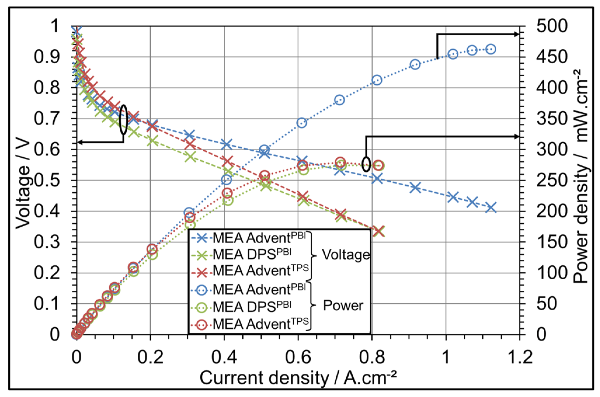
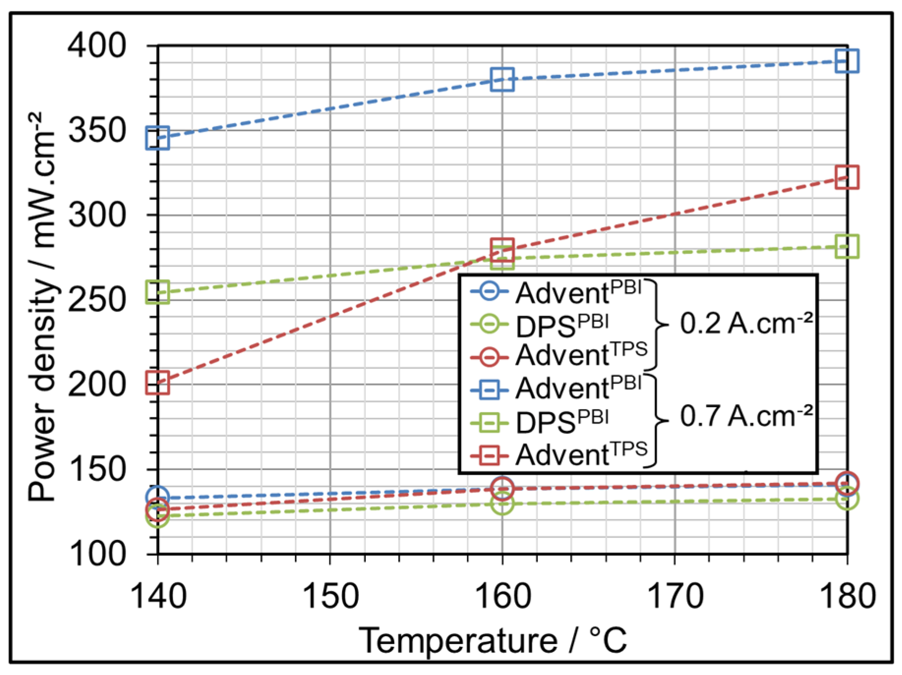
3.1. AME Comparison at Different Operating Temperatures

Figure 1 shows polarization curves of the three MEAs at 160 °C. One can see that the performances of the DPSPBI at 0.2 A·cm−2 are less than the AdventTPS, but become equivalent at 0.7 A·cm−2. However, at 0.2 A·cm−2, the AdventPBI and AdventTPS show similar performances which become significantly different at 0.7 A·cm−2 (AdventPBI ha a better performance).
Figure 2 presents the power density at different temperatures and current densities for the three MEAs. The performances and the temperature dependency of all the MEAs are closed at 0.2 A·cm−2 but significantly different at 0.7 A·cm−2. The AdventTPS shows the strongest dependence on temperature and the DPSPBI the lowest. Note that the nominal temperature of the AdventTPS is 180 °C and not 160 °C as for the two others MEAs. This can partially explain the worst performances observed at 140 °C.

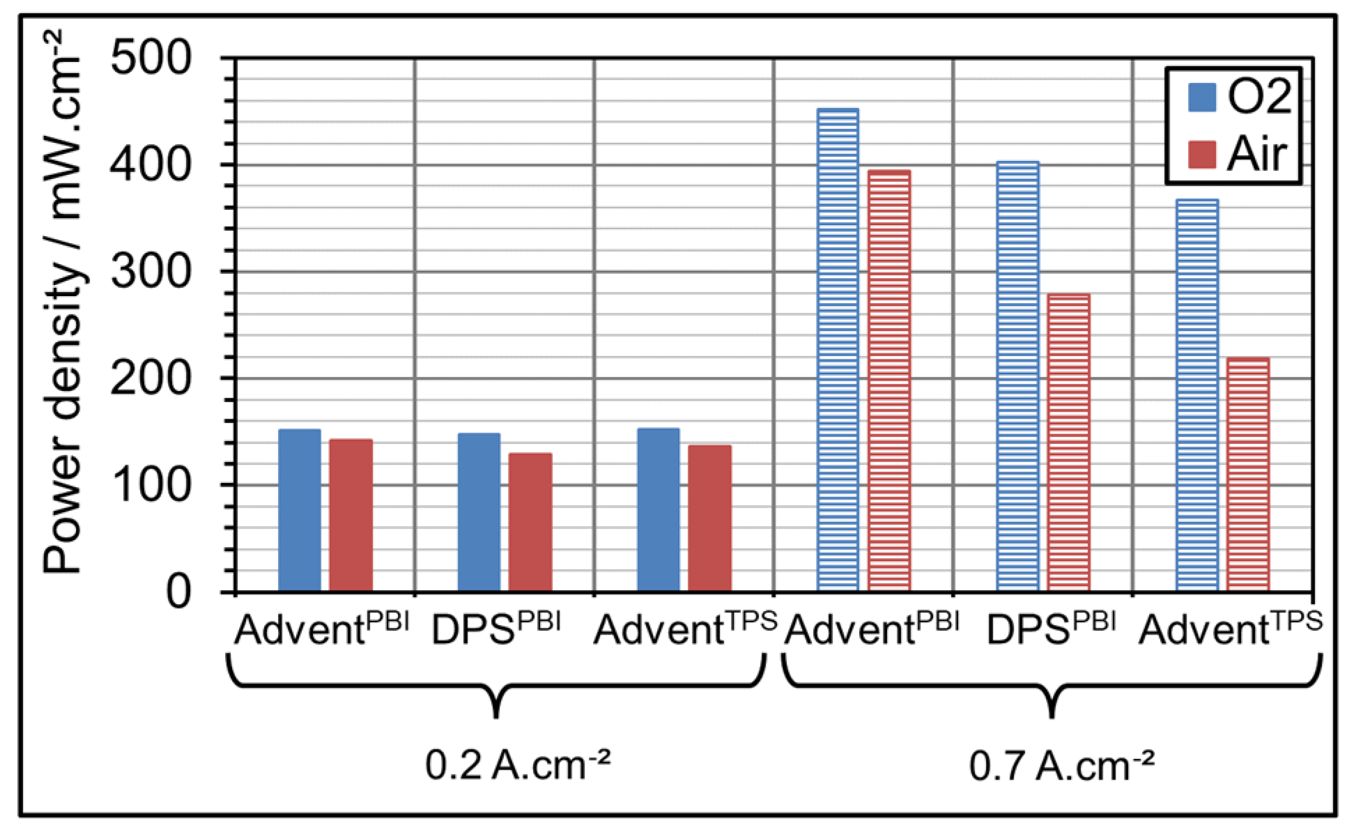
3.2. AME Comparison at Different Gas Oxidant

On Figure 3, one can see the power density of the three MEAs with different gas oxidants: air and oxygen (O2). As expected, the oxidant type impacts much more strongly the performances at 0.7 A·cm−2 than at 0.2 A·cm−2 This is consistent with a better gas diffusion with O2 than with air. Furthermore, the performances of the MEAs are more homogeneous with O2 as oxidant. This could be explained by the fact that the use of O2, reduce the gas diffusion limitation of the electrodes. Then, the structure differences between the MEAs, impacting the gas diffusion, are concealed with O2.

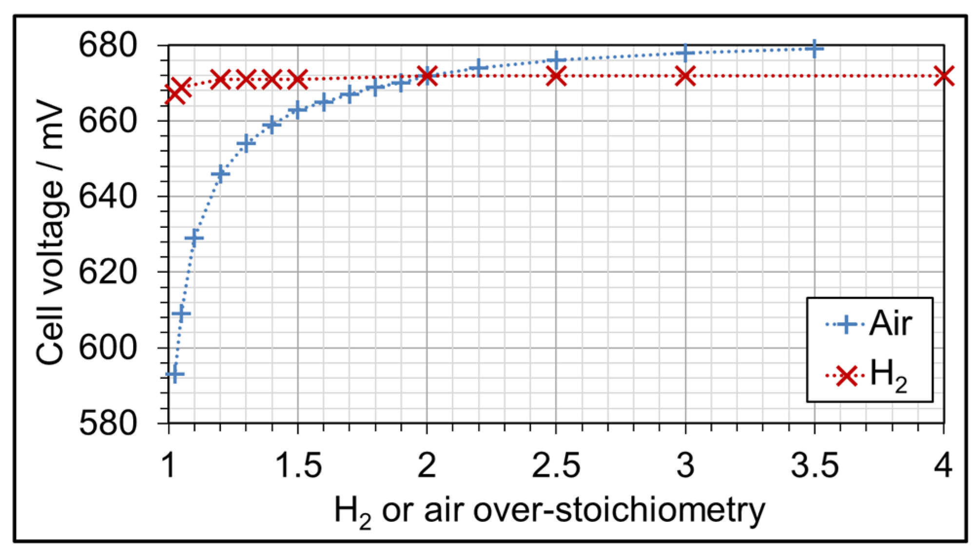
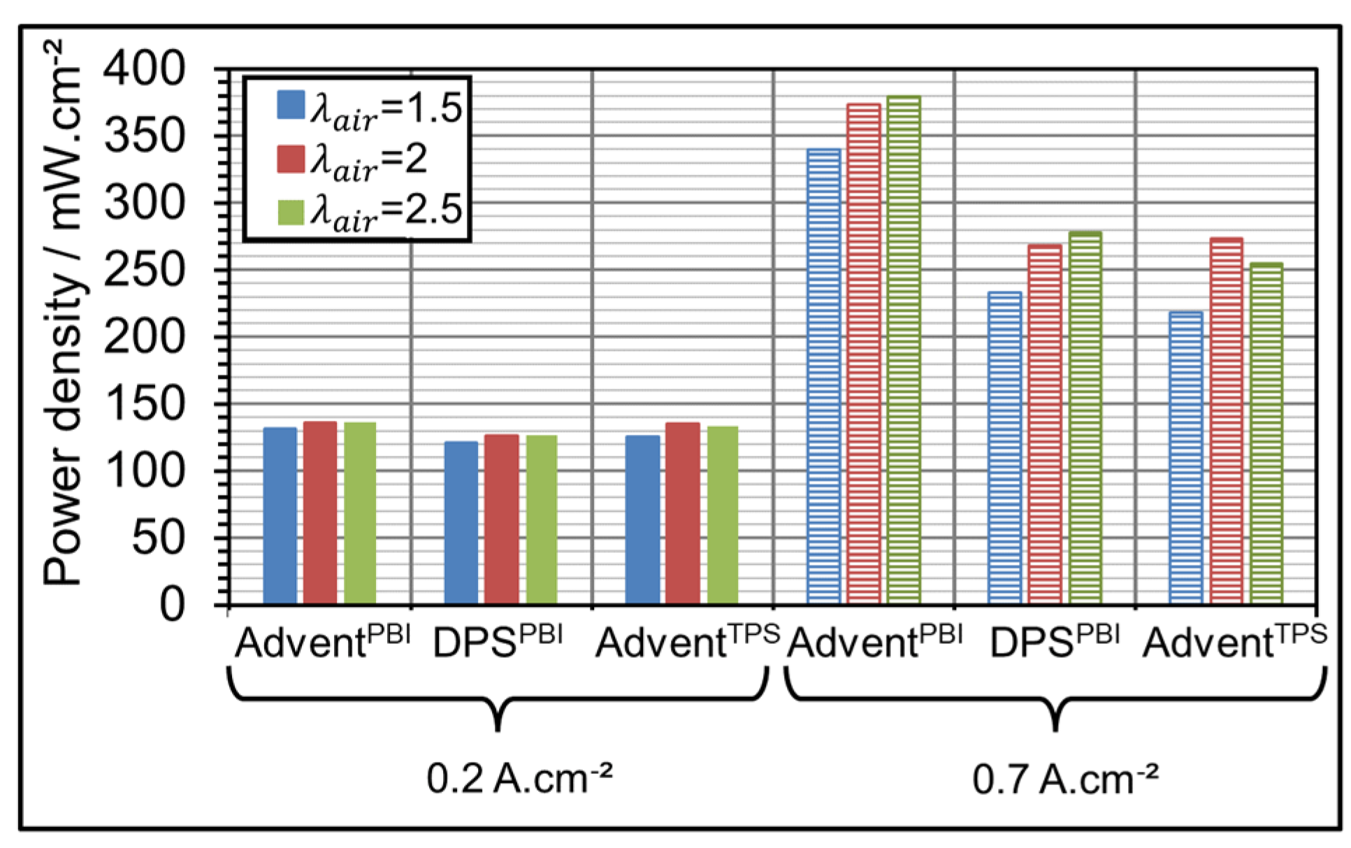
3.3. AME Comparison at Different Gas Over-Stoichiometry

Figure 4 shows the cell voltage at different air and H2 over-stoichiometry at 0.2 A·cm−2 and 160 °C with AdventPBI MEA. In one case, the H2 over-stoichiometry remains constant (at 1.20 ± 0.03) when the air over-stoichiometry varied (+symbols). In the other case, the air over-stoichiometry remains constant (at 2.00 ± 0.06) when the H2 stoichiometry varied (x symbols). One can see that the H2 over-stoichiometry ( λ H 2 ) impact appears negligible compared to the air over-stoichiometry ( λ a i r ) one within the studied variation range. In fact, between λ H 2 = 1.05 ± 0.03 and 1.4 ± 0.03 (being 29% of increase) the cell voltage increases by 0.3% (from 669 mV ± 1 mV to 671 mV ± 1 mV). On the contrary, between λ a i r = 1.05 ± 0.06 and 1.40 ± 0.06 (being 33% of increase) the cell voltage increases by 11% (from 593 mV ± 1 mV to 659 mV ± 1 mV). It must be noted as well that a saturation phenomenon seems to appear above λ H 2 = 2. This phenomenon is not observed with λ a i r in this test, even at λ a i r = 3.5.
These results concern only one current density tested (0.2 A·cm−2) and the AdventPBI MEA. Figure 5 presents the results for the three different MEA at 160 °C from the sensibility study presented in Section 2.
One can see a significant increase of the performance with the air over-stoichiometry rise at 0.7 A·cm−2. However, this increase is more important between λair = 1.5 and λair = 2 than between λair = 2 and λair = 2.5. This could signify that where is a saturation effect which is not yet reached at λair = 2.5. This is much more visible at 0.2 A·cm−2. The same conclusion can be made at 140 °C and 180 °C (results not presented).
Concerning the H2 over-stoichiometry at the three temperatures tested, the conclusions are the same as presented in Figure 4: with AdventPBI and DPSPBI, the impact is negligible compared to air over-stoichiometry because it is less than ±2 mV, which corresponds to the measurement uncertainty (results not presented). Nevertheless, this is not the case with AdventTPS, which shows variations of around ±15 mV at high current density (i.e., 0.7 A·cm−2) in the range of H2 over-stoichiometry tested. However, this behavior is attributed more to an instability of this technology at high current density and low stoichiometry than to a real sensibility on H2 over-stoichiometry. Indeed, the results (not presented here) show that the impact of H2 over-stoichiometry does not have a consistent impact on voltage (i.e., voltage does not necessarily increase with increasing over-stoichiometry), nor did we find a logical link with possible degradation during the sensitivity study. This suggests that, at high current densities, the AdventTPS may show lower voltage reproducibility than the other two technologies, which could be explained by greater voltage instability. We are not able to explain this instability, if it is really present, but it is possible that it is due to electrolyte redistribution or to the presence of acid in the electrodes or gas channels, for example.

4. Model Development

The semi-empirical and macroscopic model used in this study was initially developed by Fontès et al. [34] and further refined by Labach et al. [35] for LT-PEMFCs. Referred to as the “Basic Model” in subsequent sections, the detailed description and validation of this model can be found in a previous publication [36]. Here, all the governing equations are provided for this theoretical prediction, Equations (1)–(5), which is a steady-state model of the cell voltage, 0D, i.e., with no computation of fluid flow and isothermal.

4.1. Basic Model

4.1.1. Governing Equations

Equation (1) [33,36] provides the cell voltage model (Ucell):
U c e l l = E r e v η a c t η o h m η d i f f
with
E r e v = Δ G 0 n . F + R . T n . F l n p H 2 . p O 2 1 2
η a c t = R T α n F l n j c e l l j 0
η o h m = R c e l l . j c e l l
η d i f f = R T β n F l n 1 j c e l l j l i m
were E r e v is the cell reversible voltage, η a c t is the voltage drop linked to activation losses (charge-transfer processes), η o h m is the cell voltage drop caused by the ohmic losses (the total cell resistance taking into account ionic, electronic and contact resistances), and η d i f f is the voltage drop due to the diffusion losses (mass-transfer processes). In Equation (2), Δ G 0 represents the standard free enthalpy of water formation, R is the ideal gas constant, n is the exchanged electron’s number, F is the faraday constant, T is the fuel cell operating temperature, and p is the hydrogen or oxygen partial pressures in the gas channels at steady-state conditions. In Equation (3), α represents the charge transfer coefficient, j c e l l is the cell current density, and j 0 is the exchange current density. In Equation (4), R c e l l designates the cell total resistance measured by EIS. For currents where no EIS has been carried out, i.e., current densities below 0.022 A·cm−2, R c e l l is considered constant and its value is set to the measured one at 0.022 A·cm−2). Finally, in Equation (5), j l i m denotes the diffusion limit current density, and β is the diffusion factor [11]. Table 2 gives more details on the values of these parameters.
Note that Equation (3) is only relevant if the exchange current density is considered negligible compared to the cell current. In the present study, the magnitude order of the exchange current density is 10−5–10−6 A·cm−2 (cf. [36]), whereas the modelled fuel cell currents are higher than 5 × 10⁻³ A·cm−2. As a result, OCV and very low current densities have not been modeled. This choice is in line with PEMHT recommendations for OCV operation. Indeed, this operating mode is not recommended in order to limit carbon corrosion, which accelerates with temperature [37].

4.1.2. Model Validation

Model parameters were determined using parametric identification by fitting the model to the experimental data with a parameter identification algorithm (fully presented in [36] with a block diagram at Figure 1). The optimization algorithm used is CMA–ES (Covariance Matrix Adaptation Evolution Strategy), whose objective is to minimize the squared error between measured and modeled voltage for each current density.
This identification process is applied with a multi-polarization curve approach. In other words, the model parameters are identified using all the experimental polarization curves simultaneously. Some parameters, such as α and β , are assumed to be common to all polarization curves, while other parameters, such as j 0 and j l i m , are specific to each curve. Concerning the identification of the 27 curves in the sensitivity study (see Table 1), this results in a total of 56 parameters (a single parameter α , a single parameter β , 27 parameters j 0 and 27 parameters j l i m ). This means that only parameters j 0 and j l i m are dependent on OC variations.
The charge transfer coefficient α is presumed to depend only on the catalyst type and therefore to be independent of the OCs in the explored range. For platinum, α is typically set at 0.5 for LT-PEMFCs [35]. In our model, we have chosen to keep this parameter free, as very few typical values are given in the HT-PEMFC literature. The β parameter is linked to the reaction mechanism via the reaction order [35] and is supposed to be independent of the studied OCs. We finally assume that α and β were not affected by cell degradation during testing.
The previously described identification method using 56 parameters was applied in [36]. The obtained overall error is equal to 0.72%. This latter is calculated in two phases: (i) for all 22 current levels considered in each polarization curve, the average error is calculated, which gives 27 errors; (ii) the global error of the fitting is the average of these 27 errors. The maximum error at a given current density level is approximately 2.55%, corresponding to the polarization curve at 180 °C λH2/air = 1.35/1.5. The identified parameters show a satisfying agreement with the literature [36].
Nevertheless, the model involves the identification of four parameters for each curve. It is consequently useful for modeling existing data, and not for predicting the fuel cell voltage in untested COs. A dependence on air over-stoichiometry and a better dependence on temperature have been included in previous work [1] with the aim of addressing this limitation. In this manner, a single set of parameters common to all polarization curves can be used to model the cell voltage in the entire OC domain explored.

4.2. Final Model

With the aim of developing a model dependent on air over-stoichiometry, referred to in the following as the “Final Model”, we focus on two parameters, j 0 and j l i m , presumed to be affected by operating conditions variations.
The fine description and validation of this Final Model are described in previous work [1], and only the governing equations are given here.

4.2.1. Governing Equations

The final model is equivalent to the Basic Model, Equations (1)–(5) but the exchange current density j 0 and the diffusion limiting current density ( j l i m ) are modeled by Equations (6) and (7), respectively.
The j 0 model is taken from [1]:
j 0 = i O , r e f S c e l l p O 2 P r e f λ a i r c o e f λ a i r γ e x p E a R T 1 T T r e f
where i 0 , r e f is the reference exchange current (identified parameter without temperature dependence), S c e l l is the MEA geometric area (≈45 cm2), p O 2 represents the oxygen partial pressure along the gas channels ( p O 2   = 21,400 Pa), P r e f is the reference pressure (1 atm), γ represents the reaction order (identified parameter), E a denotes the reaction activation energy (identified parameter), T is fuel cell operating temperature, T r e f denotes the reference temperature (set here to 160 °C i.e., 433.15 K) and c o e f λ a i r is an empiric coefficient to identify (this parameter acts as a corrective coefficient of the pressure in gas channel, p O 2 , to estimate the partial pressure inside the catalyst layer, knowing the air over-stoichiometry).
The j l i m model is given by Equation (7) [1]
j l i m = n F δ D e f f T T r e f φ O 2 l n σ λ a i r λ a i r , r e f
where δ is the thickness of the cathodic GDL (400 µm for AdventPBI), D e f f is the oxygen effective diffusion coefficient (identified parameter), φ is an empirical coefficient (identified parameter), O 2 represents the concentration of oxygen in the gas channels (4.47 × 10⁻⁵ mol.cm−3 in normal conditions: 1 atm and 0 °C), λ a i r , r e f a constant ( λ a i r , r e f = 2, middle point of the sensibility study) and σ is an empiric coefficient (identified parameter).
The logarithmic dependence on λ a i r was chosen after comparing the fitting of the 27 j l i m as a function of λ a i r by a different trend curve.

4.2.2. Model Validation

With this Final Model, all the parameters are commons to all curves (see Section 4.1.2). Thus, there are only one set of parameters α , β , i O , r e f , γ , c o e f λ a i r , E a , D e f f , φ and σ , which gives a total of 9 parameters to identify.
In previous work this model was validated only with a AdventPBI MEA [1]. The identification operation applied simultaneously to the 27 polarization curves with the Final Model generates an overall error of 1.42%, and the maximum error at a given current level is approximately 18%, which corresponds to the polarization curve at 140 °C—λH2/air = 1.35/1.5 [1]. It should be noted that this polarization curve presents some unusual performances compared with those obtained at the same temperature but with different λH2. This “anomaly” is therefore attributed to reversible losses, which we are unable to explain (the next day of the test, the cell returns to “normal” performances). The second largest error obtained is equal to 15% and it is associated with the polarization curve at 140 °C—λH2/air = 1.2/1.5, which presents a notably coherent performance compared to the “anomaly” at 140 °C—λH2/air = 1.35/1.5. The overall error was twice the value reached with the base model (0.72%), and the maximum error was only 2.55% using the base model [1]. However, the Final Model requires six times fewer parameters to be identified, and all of them are common to the entire OCs area explored.
In the following section, this Final Model will be used to model the three HT-PEMFC MEAs used in this work.

5. Modelling Results

5.1. Model Accuracy on Full Sensibility Study Data

This identification process was performed simultaneously to all polarization curves (multi-VI approach) for the three MEAs independently. Thus, all OCs for each MEA were modelled alone, i.e., regardless of the other MEA data. Two model accuracy indicators are presented in Table 3.
Considering only the global accuracy indicators given in Table 3, one can see that the model is significantly more accurate on DPSPBI MEA than with the others MEAs. Table 4 shows the corresponding OCs for these two fits with each MAE. One can see that no trivial trends appear related to the OCs and the best or worst error between the MEAs.
The model parameters are also significantly different between the three MEAs but five of them ( α , γ , E a , φ , σ ) are in the same order of magnitude, whatever the MEA, as shown in Table 5. Parameters i O , r e f , c o e f λ a i r and β are less than two orders of magnitude different.
Parameter consistency is not easily judged since the Equations (6) and (7) are not often used in LT-PEMFC modelling and, to our knowledge, have never been used in HT-PEMFC.
The obtained parameter α varied from 0.34 to 0.46, which is different to the theoretical value of 0.5 generally considered for LT-PEMFCs [38]. We assume here that this parameter is independent of the operating conditions. Nevertheless, based on the literature, this coefficient is impacted by the temperature (potentially, a variation from 0.5 to 1 between 20 °C and 300 °C [53]). Furthermore, α can also be dependent on the voltage (doubling of the Tafel slope near 0.8 V [38]). This could explain why the average value of α over the entire polarization curve is not equal to 0.5 for the HT-PEMFC studied at the various operating temperatures examined in our sensitivity study. However, a supposed-constant value over the temperature range in question would seem to be a relevant approach to obtaining an acceptable level of accuracy.
The reaction order γ = 0.34–0.7, which is comparable to the values found in the LT-PEMFC literature: 0.37 to 0.52 ([39] p. 202), 0.54 [40] and 0.56 [41]. The parameter E a = 6.17 × 10⁴–8.42 × 10⁴ J·mol−1 is of the similar order of magnitude compared to some LT-PEMBT results (5.8 × 10⁴ J·mol−1 to 6.6.104 J·mol−1 ([39] p. 202), 6.7 × 10⁴ J·mol−1 [40]). Almost the same observations are made concerning i 0 , r e f = 1.27 × 10⁻³–6.31 × 10⁻⁴ A (5.25 × 10⁻⁵ A, 4.50 × 10⁻⁴ A and 4.85 × 10⁻⁴ A ([39] p. 203)), but the DPSPBI shows a significantly higher value, which is consistent with the higher platinum loading used for this MEA (1.5 mgPt·cm−2 against 0.75 mgPt·cm−2 with AdventPBI). The parameter c o e f λ a i r = 0.1–3.6 is not present in the literature and is difficult to interpret. It can be noticed that it is lower than 1 with DPSPBI and AdventTPS. This could signify a higher air over-stoichiometry dependence of j 0 .
The parameter φ = 1.24–5.98 is not the same as the literature values for LT and HT-PEMFCs; however, it is of the same order of magnitude: 1.75 [46,47], 1.5 ([48] p. 122) [49,50,51], and 1.73 to 2.07 ([52] p. 67). The parameter σ = 4.15–8.24 is not used in the state of the art. The oxygen effective diffusion coefficient ( D e f f , O 2 ) is equal to 5.37 × 10⁻⁷–5.61 × 10⁻³ cm2·s−1 different from the given value in the literature: between 1.2 × 10⁻² cm2·s−1 and 2.4 × 10⁻¹ cm2·s−1 in HT-PEMFs and around 1 × 10⁻¹ cm2·s−1 in LT-PEMFCs [27,43,44,45] with the few data found. This is the biggest disappointment with the use of this model because we are not able to explain such a deviation from the expected diffusion coefficient. This may be a sign that it is not in a global diffusion coefficient that the impact of the over-stoichiometry must be taken into account. Nevertheless, the precision of the model remains interesting. It would seem that we are paying here for our choice of having introduced an empirical correction of j l i m with a logarithmic dependence on the over-stoichiometry. This choice was led only by considerations of accuracy in the absence of a phenomenological model that could explain the dependence of j l i m on the over-stoichiometry in HT-PEMFC in the literature. In order to improve this model, it could be interesting to estimate j l i m with the Basic Model (see Section 4.1) but for a large number of over- stoichiometries and temperatures (better discretization of the domain studied) in order to hope to deduce a law of variation of j l i m as a function of the air over-stoichiometries. The choice of this law must be led both by the aim of obtaining good accuracy and by obtaining a consistent diffusion coefficient D e f f , O 2 .
In this section, two models are presented: the “Basic Model” and the “Final Model”. They both use the same equations, from Equations (1)–(5), but in the Final Model, the exchange current density j 0 and the diffusion limiting current density ( j l i m ) are modeled by Equations (6) and (7), respectively. This means that only the Final Model is able to model an air over-stoichiometry impact on cell voltage. Then, only the final model can be used to estimate or fit the data when the air super-stoichiometry varies. In the following section we will seek to test the prediction capacity of the Final Model.

5.2. Capacity of the Model to Predict Fuel Cell Performance

In the aim of studying the model’s ability to predict cell performance (cell voltage), we will shortly use the Design of Experiments (DoE) theory. In fact, the sensitivity study illustrated in Table 1 may be considered as a full factorial design including three factors and three levels. A Latin square, linked to the 9 operating conditions considered, was used as a “learning zone” in order to identify the model parameters on the associated polarization curves. Next, the remaining 18 polarization curves were estimated using the obtained parameters on the 9 curves fitting. Next, the model precision was evaluated on the 27 polarization curves obtained experimentally (more details on this evaluation are given in [1]). As in the preceding section, we calculate an overall error on 27 curves, but we are reminded that in this case, the model parameters were only identified on 9 curves.
However, modeling the 18 polarization curves not used as a “learning zone” requires precise knowledge of the value of R c e l l (see Equation (4)) for each polarization curve. In order to reduce the complexity of the problem, we have assumed that R c e l l depends only on temperature and current, and not on over-stoichiometry. In addition, it has been confirmed that the use of a single R c e l l value per temperature does not considerably decrease the model accuracy (the same global error (1.42%) is obtained as in the previous identification). Then, to model the 18 “other” polarization curves, we will use the R c e l l value from the 9 polarization curves used for fitting and consider it constant for each temperature but varying with current.
The identification process was applied simultaneously to 9 polarization curves (multi-VI approach) for the three MEAs independently. Table 6 shows two accuracy indicators obtained with the three MEAs. The global accuracy increased by 3%, 21% and 90%, respectively, for AdventPBI, DPSPBI and AdventTPS. Nevertheless, the Latin Square uses three times less curves to model 27 OCs. As with the full OCs domain, the model is more suitable for DPSPBI even for predictably. However, it must be noted that the AdventPBI shows the lowest increase of error between full domain and partial domain (Latin Square) identification.
Parameter consistency is equivalent to the one obtained with the full OCs domain as shown in Table 7. In fact, most of the parameters are in the same order of magnitude ( α , γ , i O , r e f , E a , β , φ , σ ), but this is not the case with c o e f λ a i r and D e f f with DPSPBI. This is very encouraging concerning the model predictability capacity, with sufficient parameter consistency for most of the parameters.

5.3. Advantages and Drawbacks of the Proposed Method

Compared to the Basic Model, the Final Model is able to predict the performance of the cell when the air-over stoichiometry is modified. However, the price to pay is a loss of accuracy (twice less accurate on average).
A brief comparison between 2D or 3D model using CFD methodologies and the Final Model is given in Table 8. In the table, the ‘+’ sign denotes a better capacity and ‘-’ a worse one. The Final Model is then expected to be less accurate and the parameters less consistent compared to a CFD model. However, the rapidity of the calculation is much better, which can allow the use of this model as an online diagnostics tool, for example. Furthermore, the accuracy of the Final Model is much better for medium current densities (avoiding low and high current densities), where industrial systems usually work, in order to minimize possible degradations due to low and high current densities [33,37].
This work also shows that the training domain of the Final Model used to determine the model parameter can be significantly reduced without losing accuracy at medium current densities. This also makes the model interesting for industrial application by making it possible to reduce the cost of development by reducing the number of tests to be carried out.

6. Conclusions

The sensibility study of 27 tested operating conditions allowed evaluation of the most predominant ones impacting the fuel cell voltage in steady-state (temperature and air over-stoichiometry) and to compare the behavior of three different commercially available HT-MEAs. The impact of H2 over-stoichiometry on steady-state voltage was considered negligible compared to the air-stoichiometry with AdventPBI and DPSPBI. However, this is not entirely similar to AdventTPS, which shows a significantly higher dependency on H2 over-stoichiometry.
The Final Model obtained uses only nine parameters to model the steady-state voltage, whatever the number of curves to estimate. The accuracy seems to be satisfying, with the AdventPBI and DPSPBI MEAs for industrial applications with current densities varying between 0.2 and 0.8 A·cm−2. Indeed, in order to optimize the fuel cell lifetime, it is recommended not to operate around low and high voltages (corresponding respectively to high and low current densities in HT-PEMFCs). The majority of parameter values are consistent with the state of the art, although there are few in the HT-PEMFC literature at present.
The predictability of the model was also confirmed in the explored domain throughout the sensitivity study. The model leads to a significant accuracy on 27 polarization curves by using just 9 of them to identify the model parameters. The error was 3% to 90% higher (depending on the MEA) than with the “training” on 27 polarization curves but three times fewer curves were required to identify the model parameters. This is highly motivating for industrial application, since it reduces the number of experiments and hence the cost of model development.
One should note that the model is much less accurate with AdventTPS compared to the two other MEAs tested. This could be partially explained by the fact that the MEA was significantly impacted by H2 over-stoichiometry variation (which is not the case with the PBI-based). Furthermore, the TPS®-based technology is different by the electrolyte material, which could impact the acid content within the electrodes, and then impact the charge and mass transfer processes.
This validation expands the scope of the model and the identification method (i.e., multi-VI method) to any type of HT-MEAs currently available on the market.
In further work, it will be interesting to study the impact of the hydrogen over-stoichiometry in the model in order to better model the behavior of the AdventTPS in particular.
It would also be interesting in future work to study the underlying mechanism able to explain the high impact of oxygen over-stoichiometry noted with an HT-PEMFC even if there is not liquid water. The fact that the over-stoichiometry of oxygen impacts both at low and high current density could suggest that the over-stoichiometry has an impact on oxygen concentration in the catalyst layer (as modeled in this work). Indeed, this concentration impacts both the charge and mass transfer process. which are linked in the Butler–Volmer equation (also known as Erdey–Grúz–Volmer equation) of an electrochemical reaction. However, the fact that the identified global diffusion coefficient is far from the value found in the literature could indicate that it is not relevant to attempt to model the impact of over-stoichiometry in the diffusion of oxygen. Future modeling work should take this result into account in order to determine which parameter should integrate the dependence on over-stoichiometry. In order to improve the current model, it could be interesting to estimate j l i m with the Basic Model (see Section 4.1) but for a large number of over- stoichiometries and temperatures in order have more data to determine a law of j l i m   variation against air over-stoichiometries.
In addition, it is well known that the catalyst impacts the performance of the cell [54,55]. Then, we can legitimately wonder how the catalyst (load and type of catalyst) would impact this model. To answer this question, it could be interesting to apply the method presented in this work to AMEs with different catalyst loads and/or different types of catalyst. The impact on the different parameters of the model could thus be quantified.
Finally, we believe that this kind of model could be useful for an industrial purpose, for example, where the need for fast calculation could be an important criterion and often leads to the use of a purely empirical models such as those derived from the theory of design of experiments (DoE). These purely empirical models are useful for pure voltage prediction in different operating conditions but fail to provide elements helping us to know what are the underlying physical phenomena which would explain the differences in tension between different operating conditions. The semi-empirical model developed here allows us to go a step further in terms of the interpretation of the physical phenomena involved while maintaining the simplicity and speed of a pure empirical model.

Author Contributions

Conceptualization, S.R., A.J. and C.T.; methodology, S.R., A.J. and C.T.; software, S.R.; validation, A.J., C.T., T.H., J.-B.J. and P.K.; writing—original draft preparation, S.R. and A.J.; writing—review and editing, A.J. and C.T.; supervision, A.J. and C.T. All authors have read and agreed to the published version of the manuscript.

Funding

The work was supported by IRT Saint Exupéry, SAFRAN, AIRBUS, the LAPLACE laboratory, and all the public funders (FEDER, Occitanie Region, French Government, and Toulouse Metropole) of the LAPLACE Hydrogen Platform, Toulouse, used for all tests during the FUCHYA project.

Data Availability Statement

Data are contained within the article.

Acknowledgments

The authors would like to express their sincere thanks to all the members of the FUCHYA project, namely the IRT Saint Exupéry, SAFRAN, AIRBUS, the LAPLACE laboratory, and the ANR (Agence Nationale de la Recherche). The authors would also like to thank all the public funders (FEDER, Occitanie Region, French Government, and Toulouse Metropole) of the LAPLACE, Hydrogen Platform, Toulouse, used for all tests during the FUCHYA project.

Conflicts of Interest

Author Théophile Horde was employed by the company Airbus. Author Jean-Baptiste Jollys was employed by the company Alstom. The remaining authors declare that the research was conducted in the absence of any commercial or financial relationships that could be construed as a potential conflicts of interest.

References

  1. Rigal, S.; Jaafar, A.; Turpin, C.; Hordé, T.; Jollys, J.-B.; Kreczanik, P. Steady-state voltage modelling of a HT-PEMFC under various operating conditions. Energies 2024, 17, 573. [Google Scholar] [CrossRef]
  2. FCB. BASF acquires PEMEAS. Fuel Cells Bulletin 2, 24 February 2007; p. 3. [Google Scholar]
  3. Carter, D. A Turning Point for High-Temperature PEM Fuel Cells. Fuel Cell Today Analysis 2013. Carter D. A turning point for high-temperature PEM fuel cells. Fuel Cell Today 28 August 2013. Available online: http://www.fuelcelltoday.com/analysis/analyst-views/2013/13-08-28-a-turning-point-for-high-temperature-pem-fuel-cells (accessed on 16 January 2024).
  4. Hensche, C. Celtec-P Series Membrane Electrode Assembly Technical Information Brochure; BASF Fuel Cells GmbH: Frankfurt am Main, Germany, 2010. [Google Scholar]
  5. Wainright, J.S.; Wang, J.T.; Weng, D.; Savinell, R.F.; Litt, M. Acid-doped polybenzimidazoles: A new polymer electrolyte. J. Electrochem. Soc. 1995, 142, 121–123. [Google Scholar] [CrossRef]
  6. Rahim, Y.; Janßen, H.; Lehnert, W. Characterizing Membrane Electrode Assemblies for High Temperature Polymer Electrolyte Membrane Fuel Cells Using Design of Experiments. Int. J. Hydrogen Energy 2017, 42, 1189–1202. [Google Scholar] [CrossRef]
  7. Pessot, A.; Turpin, C.; Jaafar, A.; Soyez, E.; Rallières, O.; Gager, G.; d’Arbigny, J. Contribution to the Modelling of a Low Temperature PEM Fuel Cell in Aeronautical Conditions by Design of Experiments. Math. Comput. Simul. 2019, 158, 179–198. [Google Scholar] [CrossRef]
  8. Kanani, H.; Shams, M.; Hasheminasab, M.; Bozorgnezhad, A. Model Development and Optimization of Operating Conditions to Maximize PEMFC Performance by Response Surface Methodology. Energy Convers. Manag. 2015, 93, 9–22. [Google Scholar] [CrossRef]
  9. Giner-Sanz, J.J.; Ortega, E.M.; Pérez-Herranz, V. Statistical Analysis of the Effect of the Temperature and Inlet Humidities on the Parameters of a PEMFC Model. Fuel Cells 2015, 15, 479–493. [Google Scholar] [CrossRef]
  10. Cheng, S.-J.; Miao, J.-M.; Wu, S.-J. Investigating the Effects of Operational Factors on PEMFC Performance Based on CFD Simulations Using a Three-Level Full-Factorial Design. Renew. Energy 2012, 39, 250–260. [Google Scholar] [CrossRef]
  11. Wahdame, B.; Candusso, D.; François, X.; Harel, F.; Kauffmann, J.-M.; Coquery, G. Design of Experiment Techniques for Fuel Cell Characterisation and Development. Int. J. Hydrogen Energy 2009, 34, 967–980. [Google Scholar] [CrossRef]
  12. Yu, W.-L.; Wu, S.-J.; Shiah, S.-W. Parametric Analysis of the Proton Exchange Membrane Fuel Cell Performance Using Design of Experiments. Int. J. Hydrogen Energy 2008, 33, 2311–2322. [Google Scholar] [CrossRef]
  13. Santarelli, M.G.; Torchio, M.F. Experimental Analysis of the Effects of the Operating Variables on the Performance of a Single PEMFC. Energy Convers. Manag. 2007, 48, 40–51. [Google Scholar] [CrossRef]
  14. Kregar, A.; Zelič, K.; Kravos, A.; Katrašnik, T. Educational Scale-Bridging Approach towards Modelling of Electric Potential, Electrochemical Reactions, and Species Transport in PEM Fuel Cell. Catalysts 2023, 13, 1131. [Google Scholar] [CrossRef]
  15. Li, S.; Wei, R.; Lv, X.; Ye, W.; Shen, Q.; Yang, G. Numerical Analysis on the Effect of Stoichiometric Ratio on Fuel Utilization and Performance of High Temperature Proton Exchange Membrane Fuel Cells. Int. J. Electrochem. Sci. 2020, 15, 7407–7416. [Google Scholar] [CrossRef]
  16. Oono, Y.; Fukuda, T.; Sounai, A.; Hori, M. Influence of Operating Temperature on Cell Performance and Endurance of High Temperature Proton Exchange Membrane Fuel Cells. J. Power Sources 2010, 195, 1007–1014. [Google Scholar] [CrossRef]
  17. Zhang, J.; Tang, Y.; Song, C.; Zhang, J. Polybenzimidazole-Membrane-Based PEM Fuel Cell in the Temperature Range of 120–200 °C. J. Power Sources 2007, 172, 163–171. [Google Scholar] [CrossRef]
  18. Taccani, R.; Zuliani, N. Effect of Flow Field Design on Performances of High Temperature PEM Fuel Cells: Experimental Analysis. Int. J. Hydrogen Energy 2011, 36, 10282–10287. [Google Scholar] [CrossRef]
  19. Singdeo, D.; Dey, T.; Gaikwad, S.; Andreasen, S.J.; Ghosh, P.C. A New Modified-Serpentine Flow Field for Application in High Temperature Polymer Electrolyte Fuel Cell. Appl. Energy 2017, 195, 13–22. [Google Scholar] [CrossRef]
  20. Chowdhury, P.R.; Gladen, A.C. Comparative and Sensitivity Analysis of Operating Conditions on the Performance of a High Temperature PEM Fuel Cell. Int. J. Hydrogen Energy 2024, 50, 1239–1256. [Google Scholar] [CrossRef]
  21. Waller, M.G.; Walluk, M.R.; Trabold, T.A. Performance of High Temperature PEM Fuel Cell Materials. Part 1: Effects of Temperature, Pressure and Anode Dilution. Int. J. Hydrogen Energy 2016, 41, 2944–2954. [Google Scholar] [CrossRef]
  22. Xu, B.; Li, D.; Ma, Z.; Zheng, M.; Li, Y. Thermodynamic Optimization of a High Temperature Proton Exchange Membrane Fuel Cell for Fuel Cell Vehicle Applications. Mathematics 2021, 9, 1792. [Google Scholar] [CrossRef]
  23. Søndergaard, S.; Cleemann, L.N.; Jensen, J.O.; Bjerrum, N.J. Influence of Oxygen on the Cathode in HT-PEM Fuel Cells. Int. J. Hydrogen Energy 2019, 44, 20379–20388. [Google Scholar] [CrossRef]
  24. Bayat, M.; Özalp, M.; Gürbüz, H. Comprehensive Performance Analysis of a High-Temperature PEM Fuel Cell under Different Operating and Design Conditions. Sustain. Energy Technol. Assess. 2022, 52, 102232. [Google Scholar] [CrossRef]
  25. Haghighi, M.; Sharifhassan, F. Exergy Analysis and Optimization of a High Temperature Proton Exchange Membrane Fuel Cell Using Genetic Algorithm. Case Stud. Therm. Eng. 2016, 8, 207–217. [Google Scholar] [CrossRef]
  26. Ye, L.; Jiao, K.; Du, Q.; Yin, Y. Exergy Analysis of High-Temperature Proton Exchange Membrane Fuel Cell Systems. Int. J. Green Energy 2015, 12, 917–929. [Google Scholar] [CrossRef]
  27. KP, V.B.; Varghese, G.; Joseph, T.V.; Chippar, P. Sensitivity Analysis of Operational Parameters of a High Temperature-Proton Exchange Membrane Fuel Cell. J. Electrochem. Soc. 2023, 170, 124513. [Google Scholar]
  28. Baudy, M.; Rondeau, O.; Jaafar, A.; Turpin, C.; Abbou, S.; Grignon, M. Voltage Readjustment Methodology According to Pressure and Temperature Applied to a High Temperature PEM Fuel Cell. Energies 2022, 15, 3031. [Google Scholar] [CrossRef]
  29. Wang, X.C.; Chen, J.Z.; Quan, S.W.; Wang, Y.X.; He, H.W. Hierarchical model predictive control via deep learning vehicle speed predictions for oxygen stoichiometry regulation of fuel cells. Appl. Energy 2020, 276, 115460. [Google Scholar] [CrossRef]
  30. Ziogou, C.; Voutetakis, S.; Georgiadis, M.C.; Papadopoulou, S. Model predictive control (MPC) strategies for PEM fuel cell systems—A comparative experimental demonstration. Chem. Eng. Res. Des. 2018, 131, 656–670. [Google Scholar] [CrossRef]
  31. Sisworahardjo, N.S.; Yalcinoz, T.; El-Sharkh, M.Y.; Alam, M.S. Neural network model of 100 W portable PEM fuel cell and experimental verification. Int. J. Hydrogen Energy 2010, 35, 9104–9109. [Google Scholar] [CrossRef]
  32. In-Su, H.; Chang-Bock, C. Performance prediction and analysis of a PEM fuel cell operating on pure oxygen using data-driven models: A comparison of artificial neural network and support vector machine. Int. J. Hydrogen Energy 2016, 41, 10202–10211. [Google Scholar]
  33. Rigal, S.; Turpin, C.; Jaafar, A.; Hordé, T.; Jollys, J.B.; Chadourne, N. Ageing Tests at Constant Currents and Associated Modeling of High Temperature PEMFC MEAs. Fuel Cells 2020, 20, 272–284. [Google Scholar] [CrossRef]
  34. Fontès, G.; Turpin, C.; Saisset, R.; Meynard, T.; Astier, S. Interactions Between Fuel Cells and Power Converters: Influence of Current Harmonics on a Fuel Cell Stack. IEEE Trans. Power Electron. 2007, 22, 670–678. [Google Scholar] [CrossRef]
  35. Labach, I.; Rallières, O.; Turpin, C. Steady state Semi-empirical Model of a Single Proton Exchange Membrane Fuel Cell (PEMFC). at Varying Operating Conditions. Fuel Cells 2017, 17, 166–177. [Google Scholar] [CrossRef]
  36. Rigal, S.; Turpin, C.; Jaafar, A.; Chadourne, N.; Hordé, T.; Jollys, J.-B. Steady-state modelling of a HT-PEMFC under various operating conditions. In Proceedings of the 2019 IEEE 12th International Symposium on Diagnostics for Electrical Machines, Power Electronics and Drives (SDEMPED), Toulouse, France, 27–30 August 2019; pp. 439–445. [Google Scholar]
  37. Qi, Z.; Buelte, S. Effect of open circuit voltage on performance and degradation of high temperature PBI–H3PO4 fuel cells. J. Power Sources 2006, 161, 1126–1132. [Google Scholar] [CrossRef]
  38. Mainka, J.; Maranzana, G.; Dillet, J.; Didierjean, S.; Lottin, O. On the Estimation of High Frequency Parameters of Proton Exchange Membrane Fuel Cells via Electrochemical Impedance Spectroscopy. J. Power Sources 2014, 253, 381–391. [Google Scholar] [CrossRef]
  39. Labach, I. Caractérisation et Modélisation de Piles à Combustible et D’électrolyseurs PEM a Conditions Opératoires Variables en Vue de Leur Association. Ph.D. Thesis, Université de Toulouse, Toulouse, France, 2016. [Google Scholar]
  40. Neyerlin, K.C.; Gu, W.; Jorne, J.; Gasteiger, H.A. Determination of Catalyst Unique Parameters for the Oxygen Reduction Reaction in a PEMFC. J. Electrochem. Soc. 2006, 153, 1955–1963. [Google Scholar] [CrossRef]
  41. Subramanian, N.P.; Greszler, T.A.; Zhang, J.; Gu, W.; Makharia, R. Pt-Oxide Coverage-Dependent Oxygen Reduction Reaction (ORR) Kinetics. J. Electrochem. Soc. 2012, 159, 531–540. [Google Scholar] [CrossRef]
  42. Kim, M.; Kang, T.; Kim, J.; Sohn, Y.J. One-dimensional modeling and analysis for performance degradation of high temperature proton exchange high fuel cell using PA doped PBI membrane. Solid State Ion. 2014, 262, 319–323. [Google Scholar] [CrossRef]
  43. Shamardina, O.; Chertovich, A.; Kulikovsky, A.A.; Khokhlov, A.R. A Simple Model of a High Temperature PEM Fuel Cell. Int. J. Hydrogen Energy 2010, 35, 9954–9962. [Google Scholar] [CrossRef]
  44. Hu, J.; Zhang, H.; Zhai, Y.; Liu, G.; Yi, B. 500 h Continuous aging life test on PBI/H3PO4 high-temperature PEMFC. Int. J. Hydrogen Energy 2006, 31, 1855–1862. [Google Scholar] [CrossRef]
  45. Hu, J.; Zhai, Y.; Liu, G.; Hu, J.; Yi, B. Performance degradation studies on PBI/H3PO4 high temperature PEMFC and one-dimensional numerical analysis. Electrochim. Acta 2006, 52, 394–401. [Google Scholar] [CrossRef]
  46. Scott, K.; Pilditch, S.; Mamlouk, M. Modelling and experimental validation of a high temperature polymer electrolyte fuel cell. J. Appl. Electrochem. 2007, 37, 1245–1259. [Google Scholar] [CrossRef]
  47. Chippar, P.; Ju, H. Numerical modeling and investigation of gas crossover effects in high temperature proton exchange membrane (PEM) fuel cells. Int. J. Hydrogen Energy 2013, 38, 7704–7714. [Google Scholar] [CrossRef]
  48. Zeidan, M. Etude Expérimentale et Modélisation d’une Micropile à Combustible à Respiration. Ph.D. Thesis, Université de Toulouse, Toulouse, France, 2011. [Google Scholar]
  49. Park, J.; Min, K. A quasi-three-dimensional non-isothermal dynamic model of a high-temperature proton exchange membrane fuel cell. J. Power Sources 2012, 216, 152–161. [Google Scholar] [CrossRef]
  50. Wang, Y. Modeling of Two-Phase Transport in the Diffusion Media of Polymer Electrolyte Fuel Cells. J. Power Sources 2008, 185, 261–271. [Google Scholar] [CrossRef]
  51. Wang, Y.; Feng, X. Analysis of the Reaction Rates in the Cathode Electrode of Polymer Electrolyte Fuel Cells II. Dual-Layer Electrodes. J. Electrochem. Soc. 2009, 156, B403–B409. [Google Scholar] [CrossRef]
  52. Vang, J.R. HTPEM Fuel Cell Impedance: Mechanistic Modelling and Experimental Characterisation. Ph.D. Thesis, Aalborg University, Allborg, Danemark, 2014. [Google Scholar]
  53. Kriksunov, L.; Bunakova, L.; Zabusova, S.; Krishtalik, L. Anodic oxygen evolution reaction at high temperatures in acid solutions at platinum. Electrochim. Acta 1994, 39, 137–142. [Google Scholar] [CrossRef]
  54. Fan, X.; Zhao, M.; Li, T.; Zhang, L.Y.; Jing, M.; Yuan, W.; Li, C.M. In situ self-assembled N-rich carbon on pristine graphene as a highly effective support and cocatalyst of short Pt nanoparticle chains for superior electrocatalytic activity toward methanol oxidation. Nanoscale 2021, 13, 18332–18339. [Google Scholar] [CrossRef]
  55. Yuan, W.; Cheng, Y.; Shen, P.K.; Li, C.M.; Jiang, S.P. Significance of wall number on the carbon nanotube support-promoted electrocatalytic activity of Pt NPs towards methanol/formic acid oxidation reactions in direct alcohol fuel cells. J. Mater. Chem. A 2015, 3, 1961–1971. [Google Scholar] [CrossRef]
Figure 1. Polarization curves (x symbols) and corresponding power density (o symbols) for the three MEAs (blue: AdventPB, green: DPSPBI, red: AdventTPS) at 160 °C, H2/air, λ = 1.2/2, exhausts at atmosphere.
Energies 17 03002 g001
Figure 2. Power density as a function of operating temperature for the three MEAs (bleu: AdventPB, green: DPSPBI, red: AdventTPS) at two current densities (o: 0.2 A·cm−2, □: 0.7 A·cm−2), 160 °C, H2/air, λ = 1.2/2, exhausts at atmosphere.
Energies 17 03002 g002
Figure 3. Power density for the three MEAs (AdventPB, DPSPBI, AdventTPS) at two gas oxidant (blue: Oxygen, red: air) and two current densities (filled bar: 0.2 A·cm−2, striped bar: 0.7 A·cm−2), 160 °C, H2/air, λ = 1.2/2, exhausts at atmosphere.
Energies 17 03002 g003
Figure 4. Cell voltage at different air (+, at λ H 2 = 1.20 ± 0.03) and H2 (x, at λ a i r = 2.00 ± 0.06) over-stoichiometry at 0.2 A·cm−2 and 160 °C with AdventPBI MEA (exhausts at atmosphere).
Energies 17 03002 g004
Figure 5. Power density for the three MEAs (AdventPB, DPSPBI, AdventTPS) at three air over-stoichiometries (blue: λ a i r = 1.5, red: λ a i r = 2, green: λ a i r = 2.5) and two current densities (filled bar: 0.2 A·cm−2, striped bar: 0.7 A·cm−2), 160 °C, H2/air, λ = 1.2/2, exhausts at atmosphere.
Energies 17 03002 g005
Table 1. Range of variation of the three parameters considered in the sensitivity study.
Parameter SymbolMinimum ValueMedium ValueMaximum Value
λH21.051.21.35
λair1.522.5
T140 °C
(413.15 K)
160 °C
(433.15 K)
180 °C
(453.15 K)
Table 2. List of model parameters. A parameter whose value can vary as a function of current or OCs is called a Variable (measured or calculated), a parameter whose value is invariable is named a Constant (experimentally measured or from the literature), and a parameter required to adjust the model from experimental results is named a Fitting Parameter, which can depend (one parameter per polarization curve) or not (one parameter common to all polarization curves) on the OCs.
ParameterTypeValue
Δ G 0 VariableCalculated
n Constant2
F Constant96,485 C·mol−1
R Constant8.314 J·mol−1·K
T VariableMeasured
p H 2 ConstantMeasured: 102,100 Pa absolute
p O 2 ConstantMeasured: 21,400 Pa absolute
  j c e l l VariableMeasured
j 0 Fitting ParameterOCs dependent
α Fitting Parameternon-OCs dependent
R c e l l VariableMeasured
j l i m Fitting ParameterOCs dependent
β Fitting Parameternon-OCs dependent
Table 3. Global accuracy indicators for the three MEAs.
ErrorAdventPBIDPSPBIAdventTPS
Overall error a (%)1.421.072.11
Maximum error b (%)18/15 c618
a: The global average error presented in Section 4.1.2. b: The maximum error at a given current level. c: The maximum error at a given current level without considering the “anomaly” OC, i.e., at 140 °C—λH2/air = 1.35/1.5 (Section 4.2.2). Only consistent with the AdventPBI MEA tested.
Table 4. OCs related to the best and worst fits for the three MEAs.
FitAdventPBIDPSPBIAdventTPS
Best fit160 °C—λ = 1.05/2.5140 °C—λ = 1.35/2180 °C—λ = 1.2/2.5
Worst fit a140 °C—λ = 1.2/1.5140 °C—λ = 1.2/1.5140 °C—λ = 1.05/2.5
a: Second worst fit with AdventPBI, because the worst fit correspond to “anomaly” OC, i.e., at 140 °C—λH2/air = 1.35/1.5 (Section 4.2.2).
Table 5. Model parameters after identification in full sensibility study.
ParameterAdventPBIDPSPBIAdventTPSLiterature
α 0.460.340.400.5 [38]
γ 0.470.340.700.37–0.56 [39,40,41]
E a (J·mol−1)8.42 × 1046.17 × 1047.43 × 1045.8 × 104–6.7 × 10⁴ [39,40]
i O , r e f (A)5.62 × 10−41.27 × 10−36.31 × 10−45.25 × 10−5–4.85 × 10⁻⁴ [39]
c o e f λ a i r 3.601.21 × 10−11.00 × 10⁻¹/
β 1.08 × 10−18.31 × 10−22.55 × 10⁻²/
D e f f (cm2·s−1)5.61 × 10−32.37 × 10−71.06 × 10−61.2 × 10−2–2.4 × 10⁻¹ [42,43,44,45]
φ 1.971.245.981.5–2.07 [46,47,48,49,50,51,52]
σ 4.328.244.15/
Table 6. Global accuracy indicators for the three MEAs with Latin Square.
ErrorAdventPBIDPSPBIAdventTPS
Overall error a (%)1.461.294.02
Maximum error b (%)30/8 c721
a: The global average error presented in 4.1.2. b: The maximum error at a given current level. c: The maximum error at a given current level without considering the “anomaly” OC, i.e., at 140 °C—λH2/air = 1.35/1.5 (Section 4.2.2) Only consistent with the AdventPBI MEA tested.
Table 7. Model parameters after identification on Latin Square.
ParameterAdventPBIDPSPBIAdventTPSLiterature
α 0.470.350.650.5 [38]
γ 0.440.271.200.37–0.56 [39,40,41]
E a 8.60 × 1045.86 × 1041.94 × 1045.8 × 104–6.7 × 10⁴ [39,40]
i O , r e f 7.30 × 10−43.24 × 10−32.39 × 10−45.25 × 10−5–4.85 × 10⁻⁴ [39]
c o e f λ a i r 8.833.702.08 × 10−1/
β 1.04 × 10−17.96 × 10−23.98 × 10⁻³/
D e f f 5.66 × 10−34.96 × 10−11.98 × 10−61.2 × 10−2–2.4 × 10⁻¹ [27,28,29,30,31,32,33,34,35,36,37,38,39,40,41,42,43,44,45,46,47,48,49,50,51,52,53]
φ 4.401.756.101.5–2.07 [46,47,48,49,50,51,52]
σ 1.8010.5726.02/
Table 8. Model comparison with multi-dimensional model.
Topic2D-3D ModelFinal Model
Parameter consistency+
Accuracy+
Fast calculation+
Disclaimer/Publisher’s Note: The statements, opinions and data contained in all publications are solely those of the individual author(s) and contributor(s) and not of MDPI and/or the editor(s). MDPI and/or the editor(s) disclaim responsibility for any injury to people or property resulting from any ideas, methods, instructions or products referred to in the content.

