Abstract
The successful implementation of predictive maintenance for offshore wind farms suffers from a poor understanding of the consequential short-term impacts and a lack of research on how to evaluate the cost-efficiency of such efforts. This paper aims to develop a methodology to explore the short-term marginal impacts of predictive maintenance applied to an already existing preventive maintenance strategy. This method will be based on an analysis of the performance of the underlying predictive model and the costs considered under specific maintenance services. To support this analysis, we develop a maintenance efficiency measure able to estimate the efficiency of both the underlying prediction model used for predictive maintenance and the resulting maintenance efficiency. This distinction between the efficiency of the model and the service results will help point out insufficiencies in the predictive maintenance strategy, as well as facilitate calculations on the cost–benefits of the predictive maintenance implementation. This methodology is validated on a realistic case study of an annual service mission for an offshore wind farm and finds that the efficiency metrics described in this paper successfully support cost–benefit estimates.
1. Introduction
The Levelized Cost of Energy (LCOE) for wind energy is becoming increasingly competitive within the energy sector [1,2]. LCOE measures energy production relative to overall costs, with improvements coming from increased production or decreased Operational Expenses (OpEx) and Capital Expenses (CapEx). Onshore wind energy maintains a lower LCOE than offshore wind, partly due to higher Operations and Maintenance (O&M) costs [3], as logistics and operations are more complex for offshore projects. Since O&M accounts for about 20% of total wind energy costs, improving this area is crucial to lowering offshore wind LCOE.
O&M operations for Wind Farms (WFs) involve optimizing logistics, supply chain management, failure diagnostics, and maintenance. All Wind Turbines (WTs) are equipped with Supervisory Control And Data Acquisition (SCADA) systems that collect high-frequency operational data. Increasing interest in using these data for predictive maintenance aims to further optimize WF maintenance [4], though there is limited research on its cost-effectiveness.
Predictive maintenance is a well-described topic in the literature, and it has many cases of successful implementation in several different industries [5,6,7]. Predictive maintenance typically consists of two main elements: a prediction model itself and a service planning model. The prediction model, often based on machine learning algorithms, is designed to learn patterns from historical data on WT downtime events and predict future downtime occurrences. These downtime events are any internal issues the WT experiences that require a shutdown of the WT operations, remote restart, and in some cases, manual corrective maintenance to restart the WT. These unplanned downtime events and the associated availability loss present a large production value loss [8,9].
The service planning model is responsible for considering the available maintenance resources (vessels, service teams, etc.), related costs, and the risk information from the prediction model, and creating the service schedule with respect to routing. By understanding the relationship between the prediction model and the service planning model, the benefits of predictive maintenance can be better understood and evaluated on a case-by-case basis. This, in turn, will provide a more comprehensive understanding of the impacts predictive maintenance can have on existing O&M strategies.
While studies such as [10] suggest that the potential for predictive maintenance to reduce WF life-cycle costs is high, its actual implementation is not a comprehensive overhaul of the maintenance strategy but rather consists of several incremental changes to often pre-existing maintenance operations. In this research, this approach for O&M improvements to a specific maintenance operation will be investigated. The marginal impact of predictive maintenance will be compared with existing preventive maintenance solutions to evaluate the cost–benefits. The primary contribution of this work is a methodology for evaluating specific maintenance operations for Offshore Wind Farms (OWFs) concerning the implementation of predictive maintenance. This continues previous research by the authors, which focused on developing specific reference models for predictive maintenance [11,12], where service mission planning was the focus of the work and not the monetary impact.
This paper is organized in the following way. Section 2 explores related works within LCOE improvements for wind energy and identifies relevant research gaps, while also introducing the concepts of maintenance relevant to this paper. Section 3 introduces the problem formulation and states the cost functions that the results of this paper are based on. The predictive maintenance methodology is stated in Section 4, exploring both the predictive model and the service planning model. Section 5 formulates the efficiency factor, and this is validated by a numerical case study in Section 6. Section 7 and Section 8 consist of a discussion of the results of the paper and a conclusion.
2. Background
2.1. State of the Art
The most common measure for comparing sources of energy is the LCOE, which is the ratio of lifetime OpEx and CapEx to total lifetime energy output. During the first several decades of wind energy development, the LCOE decreased impressively [13]. Most of these improvements stem from increases in individual WTG size, rotor diameter, and nominal power output, as well as overall WF sizes [14], which all directly enhance the productivity of wind energy while only increasing overall expenditures at a relatively lower rate. This is particularly true for offshore wind energy compared with onshore [15], leading to comparatively increased interest in offshore wind despite its overall lower LCOE. While this trend is expected to continue [14,16], other solutions for decreasing LCOE are also being explored through cost-lowering strategies.
The overall cost of wind energy consists of approximately two-thirds CapEx, including costs related to project development, decommissioning, and financial expenses [3]. While the WT itself has become more expensive recently due to rising commodity prices and higher interest rates [17,18], efforts are ongoing to improve other aspects of CapEx. The increased popularity of green financing [19], the derisking of wind development projects [20], and the creation of wind energy project auctions [21] are all contributing to a better financial situation for the wind industry.
The number of WFs nearing their end of life is increasing [22], leading to greater scrutiny of the decommissioning phase and interest in improving the overall life-cycle costs of the WT. Since WT blades are the largest components, sustainable and recyclable blades are being developed [23]. Other blade materials are being analyzed for their recyclability and increased circularity [24]. Some WFs have not experienced the level of stress that the WTs were designed for, enabling lifetime extensions and increasing the useful life of these sites [22]. Similarly, designs are being made to improve the natural lifetime of the towers [25].
However, most CapEx optimizations will only be performed once for each new WT. Improvements in WT installation, project development, and design enhancements can only be applied to future wind energy projects and will not benefit existing WFs. This is not the case for end-of-life improvements, but these are also one-time improvements for the decommissioning phase.
On the other hand, OpEx covers one-third of the total costs considered in the LCOE of offshore wind energy [3], and improvements to OpEx operations can be applied more widely and readily. Any enhancement in an OpEx process can be implemented in existing WFs and may also compound throughout the WF’s lifetime, given that the process is performed continuously. This applies to general maintenance and servicing of the WFs. Additionally, by optimizing the maintenance of the WFs, the reliability, availability, and productivity improve, further enhancing the LCOE.
Given the significant share of OpEx in the LCOE of wind energy, it is a prime target for cost reduction and optimizations, which has been steadily occurring for onshore wind energy [26]. While the overall OpEx developments for offshore wind energy are less clear [17], there certainly seems to be potential [27,28]. This is due to the significant differences in OpEx between sites caused by varying complexities of operations among OWFs, and the generally low availability of information on OpEx for offshore wind projects. This further emphasizes the need for a generalized approach to predictive maintenance evaluation that can be applied across the diverse operational conditions of OWFs.
OpEx most often consists of cost elements related to O&M, insurance, land rent, taxes, and management [29]. Of these, O&M is by far the single largest expenditure, taking up to 60% of total OpEx [3,30], being comparatively higher for offshore wind energy because of offshore logistical complexity [31]. O&M is also the most readily improvable aspect, as it consists of many separate processes, like the supply chain of spare parts, general maintenance, WT operations, etc. Each of these can provide optimization opportunities.
Tendencies within improvements of O&M for wind energy follow the traditional methodology for O&M regimes. Many improvements are gained from improved reliability through condition monitoring and maintenance optimization [32]. Through increasingly sophisticated sensor technology, inspection techniques, and data acquisition systems, operators have better control over the assets and can improve maintenance operations. An example is the inspection of blades’ surfaces by drone and utilizing computer vision models for the detection of blade faults [33,34,35]. Similarly, simulation models of erosion of the blade leading edge are developed to improve protection of blades [36], and prognostic failure models are developed for internal components [37,38]. Less specific and more top-down risk-based maintenance frameworks are designed in [39,40].
While the data collection and analysis have improved markedly, improvements to the actual logistics and supply chain management are in focus as well [41]. For OWFs, this is especially the case because of the complex logistics [42]. In [43], a spare parts inventory is optimized in tandem with an O&M strategy, and a strategic level preventive maintenance and planning system is described considering several objectives in [44,45], where elements such as costs and reliability are optimized by considering asset degradation over time and failure rates. When planning the schedule for a specific maintenance campaign, several methods and approaches are available [46], and examples can be found in [11,47]. While the methods are well described, the impact and benefits they can provide are evaluated from a strategic life-cycle perspective or are not considered at all.
Taking all the above into account, it is clear that efforts are put into improving the LCOE of wind energy in many different ways; however, we identified the following research gaps on the topic of predictive maintenance for OWFs. While there are separate and numerous sources for both predictive/preventive/reactive maintenance applications for OWFs, there is a poor understanding of how to apply these approaches in tandem. In particular, we found that the available strategic life-cycle cost analysis on the implementation of predictive maintenance suffers from a lack of knowledge of the short-term cost–benefits of predictive maintenance. Because of these gaps, we seek to investigate a specific methodology aimed at formulating a short-term cost–benefit analysis approach associated with predictive maintenance strategy implementation. Furthermore, while the risk-based maintenance strategies are explored from a macro perspective in the literature, this methodology will be validated in a case study of service mission planning with pre-existing preventive maintenance to better present the marginal impacts of predictive maintenance.
2.2. Maintenance Strategies
Three archetypes of maintenance strategies exist for maintaining OWFs [48,49,50], which can also be mixed in their actual implementation. These are reactive, preventive, and predictive maintenance.
Reactive maintenance in OWFs involves responding to equipment failures or malfunctions that occur unexpectedly. This may include repairing damaged components, replacing faulty parts, or addressing issues arising from unforeseen events such as severe weather or equipment breakdowns. Since it involves emergency situations, it is never planned. The advantage is that there is a low likelihood of unnecessary maintenance, and the amount of maintenance is kept to a minimum. Moreover, the implementation of reactive maintenance is easy. However, the disadvantages include longer downtimes, the potential for more severe failures, the requirement for having spare parts always available, the need for teams and vessels to always be on standby, and potential damage to secondary components. These disadvantages make this maintenance strategy very expensive.
Preventive maintenance in OWFs involves regular prescheduled inspections, servicing, and upkeep of the WTs and associated infrastructure. This includes tasks such as checking for corrosion, inspecting blades for damage, testing electrical components, and performing scheduled maintenance activities to ensure that the WTs are operating efficiently and reliably. Maintenance operations are preplanned on a set time basis, such as every year, allowing for better scheduling based on available weather windows, vessel fleet, and service teams’ availability. Furthermore, preventive maintenance is best utilized once failure rates are known, and average failure intervals can be predicted accurately. If the interval is too short, it results in increased operational costs, wasted production time, and unnecessary replacements of components in good condition. Conversely, if the interval is too long, unexpected failures could occur between maintenance operations, requiring reactive maintenance.
Predictive maintenance in OWFs utilizes data from sensors, monitoring systems, and historical operational data to predict potential equipment failures before they occur. This maintenance strategy involves analyzing trends in WT operations and failures for specific WTs, monitoring key parameters such as vibration, temperature, and oil conditions, and using predictive analytics algorithms to forecast when maintenance is needed. Consequently, since the nature of the problem is known beforehand, the proper spare parts and appropriate tools can be brought to the WT, resulting in minimal downtimes as the repair is scheduled before a complete malfunction. The disadvantages of predictive maintenance include the need for sensor technology and the potential for poor predictive modeling leading to false alarms and over-maintenance. Furthermore, it should be noted, that smart sensing demands online communication based on wireless technologies between the monitoring station and the WT, so the current conditions and operations of the WT can be received.
3. Problem Formulation
3.1. Costs and Profit
When studying the short-term cost-effectiveness of maintenance strategies, many elements of LCOE are not necessary and can be disregarded. This study will simplify the formulation of profitability from a short-term maintenance-centric perspective. As such, the profit numbers themselves are not precise, but the changes in costs and profit numbers are relevant to the cost–benefit analysis. This makes the approach less accurate and realistic but much more relevant to study the dynamics related to the cost–benefits of predictive maintenance strategies.
Figure 1 shows the overall dynamics of predictive maintenance. While introducing additional costs in the form of increased complexity to the existing maintenance operations and development of the prediction models, it is expected that the increasing reliability/availability of the WTs will lead to less maintenance costs in the future and an immediate and sustainable increase in production [10].
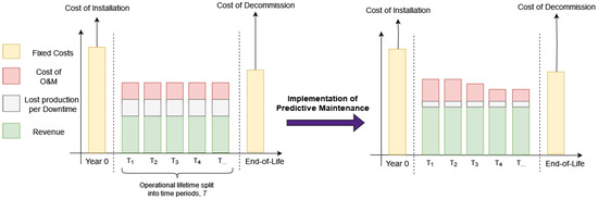
Figure 1.
Assumed cost–benefits of predictive maintenance in the long term. The short-term perspective is for each separate time period T.
For any time period T, the operational profits can be represented by the following equation:
where is the potential revenue from the produced power, and is the cost of downtime. is thus the actual revenue gained from the produced power. is the cost of service, and is the cost of predictive services. collects all costs related to the maintenance operations, such as planning of maintenance, logistics, spare parts, technician salary, etc. Fewer vessels and service teams will decrease , at the expense of the service capabilities. consists of all additional costs related to predictive maintenance that are not included in . These costs are related to the development of the prediction model, computation and databases, and model maintenance. will increase as better performing model performance is sought, which will in turn provide the most benefits. While and are highly specific to individual use cases and cannot be formulated clearly, and can be stated as
where is the steps of consideration. is the nominal power output of the , is the price of energy at time t, and is the wind factor, which is what percent of the nominal power output can be generated given the wind speeds at time t. The multiplication of is a discount rate based on industry availability standards regularly used when calculating the value of WT power output [51]. D is a downtime event, h is the average length of a downtime event in hours, and is the set of all downtime events. Parameters such as wind speeds and energy prices are also not under the control of maintenance strategies, and while they can be included in the cost formulations, they are initially assumed static on a case basis for simplification and clarity. With these definitions in place, we can now see how they relate to predictive maintenance.
3.2. Cost Efficiency of Predictive Maintenance
A simple visual representation of our predictive maintenance methodology can be seen in Figure 2. This showcases the full predictive maintenance process that we are interested in implementing, from the beginning with data collection to the actual service planning model. Note that the service planning model without the prior elements is simply the preventive maintenance that is already being performed in the form of an annual service mission for a selection of WTs. As such, this predictive maintenance process can be seen as a better-informed version of preventive maintenance.
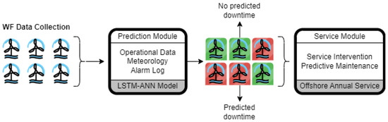
Figure 2.
A graphical representation of the overall predictive maintenance process.
The first element of Figure 2 shows a WF with ongoing data collection. How these historical data are used in training machine learning models is explained in Section 5.1. The resulting prediction model will generate predictions of general WT downtime events; there will either be a downtime event during the service mission or the WT will be operationally safe. The service planning will then be supported by this information to optimize the maintenance. How this optimization is achieved is explained in Section 5.2. To explore the cost–benefits of this additional information and the extension from preventive to predictive maintenance, we need to understand how this relates to the costs and profit.
When assessing the benefits of predictive maintenance, the prediction model performance is highly influential. A badly performing prediction model will have no ability to improve maintenance beyond preventive maintenance, and in the worst case will be an overall disadvantage. The more precise the model becomes, the potential impact it can have will increase as well. This prediction efficiency will be represented by
where . As is tradition in mathematics, we then seek to minimize , which means the performance of the model increases. An of 0 means that the model will correctly predict all imminent downtime events for the total OWF, and as increases the model becomes worse at predicting the downtime events.
Depending on the service capabilities and maintenance strategies, the potential impact of predictive maintenance will vary. Even with a perfect prediction model, if the service mission suffers from limited capabilities, the actual impact of predictive maintenance will be limited as well. To capture the maintenance efficiency, is reformulated as
where . A more exact presentation of these formulations for and is stated in Section 6. If we include these efficiency measures in Equation (1), we obtain
From Equation (6), we can now see which costs are influenced by the efficiency metrics. impacts , as a better-performing model will require more effort and resources to train. The other costs are influenced by instead, as these are dependent on the performed service maintenance. A higher will in turn lead to higher , as the predictions are improving the service mission. It must also be noted that is not associated with either efficiency metric, as this is the potential revenue of the WTs and will not change no matter the efficiency of maintenance. Only the realized revenue will increase through a decrease in following a maintenance efficiency increase. and are functions of , as these costs are only impacted by changes to maintenance. The counterintuitive increase in with increasing compared with life-cycle perspective studies of predictive maintenance, which indicate that the cost of service should decrease, is due to the increasing complexity of service operations being performed in the short-term. The short-term benefits of predictive maintenance come entirely from decreasing the operational downtime of the WTs. Predictive maintenance can only be cost-effective in the short term when decreases more than and increases, and the evaluation of this balance is not a trivial task.
From this, the problem statement can be formulated as follows:
“Does there exist such an evaluation methodology of the short-term cost–benefits by the implementation of prediction maintenance applied to existing preventive maintenance strategies?”.
The main contribution of this work will be to explore this evaluation method by the use of and , how they may be defined, and how they can be used to evaluate the efficiency of predictive maintenance on a case basis. By creating this method, we support the domain knowledge of applied maintenance strategies and how they can improve WF reliability, improve offshore wind LCOE, and provide a slight increase in overall green energy production.
4. Predictive Maintenance Methodology
To describe the predictive maintenance methodology in detail, it is necessary to first understand the service mission that it is designed for and will be applied to. This is the annual service mission, which is often a contractual necessity for the service providers of an OWF. The service provider will visit and perform an examination of the overall health of the WTs once per year, possibly only for a subset of the total WTs. This will identify major issues and failures in the WT and ensure overall operational health. However, as WFs consist of several WTs that must be serviced within the same service mission, the planning of the mission reveals some points readily available for optimization.
Firstly, as the annual service is designed in part to ensure WT operational health, there is a benefit to prioritizing WTs with higher than average risk of downtime events. To identify these WTs, the prediction model will learn the signal for imminent WT downtime events and estimate the risk thereof. The assumption is that a service visit will prevent the downtime event and avoid the loss of energy production during this downtime event. There will be an underlying risk of experiencing even after the visit; however, this can be assumed to be equal for all WTs and therefore can be ignored as an unchanging constant that does not impact the service planning. Secondly, the specific schedule for the service mission must be planned. This action consists of several considerations on logistics, and the optimal planning of this along with the prioritization of the high-risk WTs is handled in the service planning model.
The predictive maintenance methodology of this project consists of two processes, the prediction of high-risk WTs and the planning of the service mission, which is reflected in Figure 2. Both of these processes must be highly specialized for this service mission, and while this paper works with this specific case study of the annual service mission, this general setup can be transferred to any other maintenance operation as well. Below is a detailed description of the processes and how they are designed for the annual maintenance mission.
4.1. Prediction Model
The prediction model is built on deep learning methods applied to data collected from several thousands of WTs of different types and under different conditions. A sketch of the training process can be seen in Figure 3, which mirrors methods used in other literature [52,53,54]. The training data consist of SCADA data that are specific to the WTs. This contains information on recent operation behavior like power output, loads, yaw and pitch, etc. Meteorological data for the WF are utilized as well, which contain both recent and forecasted features such as wind speeds, wind gusts, humidity, precipitation, temperatures, etc. A single training sample consists of all these data in an hourly sequential format for the last week and a week of meteorological forecasts, which are merged, transformed, and normalized in preprocessing before they can be used for training.
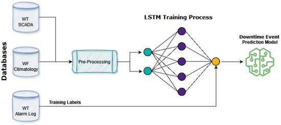
Figure 3.
A flowchart of the training process of the prediction model. The visualized neural network is not the actual architecture but a general representation of a neural network.
For supervised learning, training labels are required, and this is provided by the WT alarm logs. This is a binary categorical value, as either the WT will experience a downtime event or it will not. Taking the sequential nature of the data into account, the prediction model itself is a Long Short-Term Memory (LSTM). This is a recurrent neural network, which is well designed to deal with the sequential data formats while still being able to output binary/categorical predictions with the sigmoid activation function as the output neuron. This is understood to currently be among the best-performing methods for similar tasks [55,56,57].
For each data sample, i, there is an associated label, , where the true labels are categorical. In this paper, the labels are if the WT will not experience an imminent downtime event or if there is an imminent downtime event. We are using the term imminent here as the exact time frame of the predictions is adjustable to the specific use case of the model and must be decided in the training phase of the model. The output of the model is the prediction score of a sample, i, , which in a binary classifier will be collapsed into prediction labels by a certain threshold, most often . In Section 6, it is explained that this threshold collapse is not ideal when using such prediction models for decision support.
For each prediction, there is also the prediction of the opposite event. For example, given a prediction score of , the opposite event prediction score is . This becomes relevant later on as the opposite event prediction must be considered, instead of collapsing into binary labels. For ease of reading, from this point onwards, the notation of will be simplified to , and the opposite event prediction score will always be expressed as .
Given a series of predictions with known labels, the quality of the model can be assessed. The model quality assessment in this paper is similar to ordinary model performance assessments but with the addition and the process of derivation. Ordinary machine learning methods are focused on training the best-performing model and thus are centered around performance metrics designed to compare models. This means that the precise prediction scores are collapsed into classification labels, and these are used to calculate performance metrics and compare models. However, when the output of such models is used in decision support systems, such as predictive maintenance, more nuance is necessary. Such nuance is based on the assessment of the quality of individual predictions, i.e., how confident was the prediction score compared with the true label. The quality of all predictions will determine the model’s , which is not only a metric that serves to explain the quality of the model, but with the right formulation, will also help understand how it can support predictive maintenance.
4.2. Service Planning Model
The probability of downtime occurrence for each WT (and the associated cost ) in the considered period of time T, forecasted in the prediction process (i.e., predictive maintenance), constitute input data for the service mission planning process (hereinafter referred to as ). The mission of interest is in this case the annual service visit, where it is expected that all WTs under consideration are visited and serviced. Knowing which WTs are characterized by a high probability of , you can plan a service mission in such a way as to prioritize them and prevent the upcoming risk of downtime. The service mission includes the allocation of available service teams to selected WTs and their transport using the available fleet of vessels. In the adopted planning process for this type of mission, the following assumptions were made [12]:
- Each WT is serviced by one service team (service team number is limited to );
- Service teams are transported to WTs using a fleet of vessels (V);
- Each WT is visited by vessels twice: the first time to deliver the team, the second time to pick up the team;
- The service time of each WT is known, and the transport times between WTs are also known;
- Depending on the adopted strategy, the service team delivered to the WT by a given vessel must be collected by that vessel or may be collected by another one.
Depending on the number of WTs requiring servicing, service missions last from one to several days. This means that the missions are subdivided into a sequence of one-day sub-missions , carried out on subsequent days of the considered period T: ), where denotes the number of sub-missions (number of mission days).
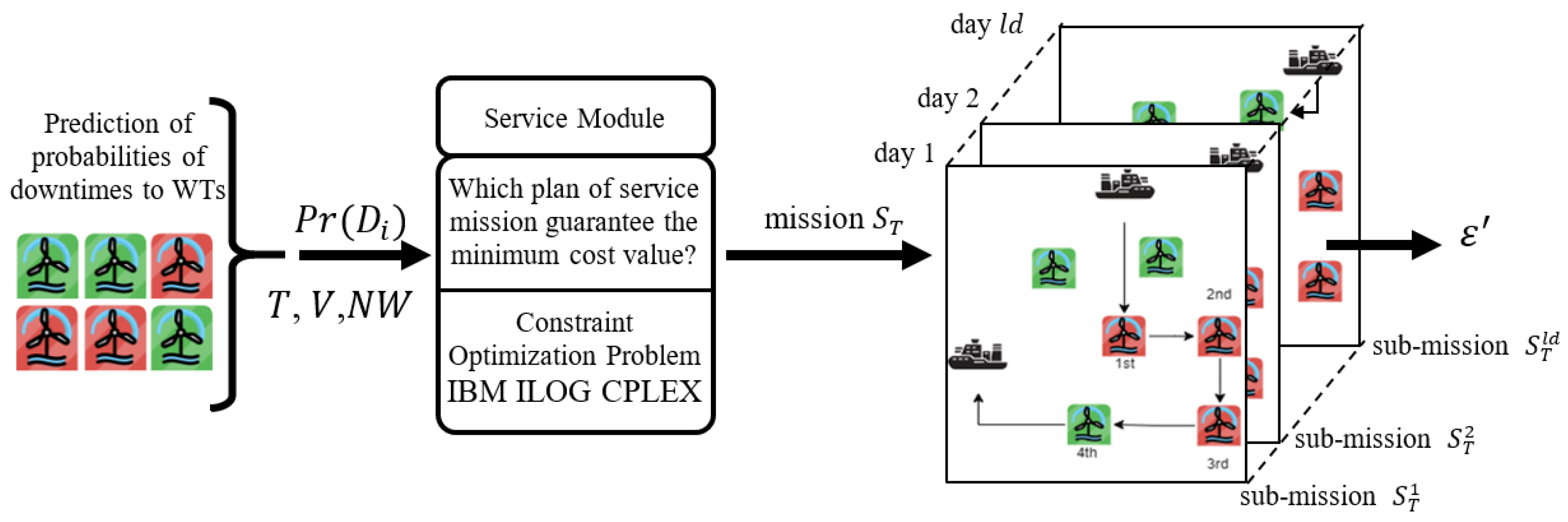
In general, there may be many different service mission plans depending on the number (and type) of vessels used, service teams, and service strategies adopted. The adopted plans may result in different number of mission days which determine the value maintenance efficiency . Under predictive maintenance, planning service missions comes down to determining an plan whose value of guarantees the lowest maintenance costs (6). Declarative programming techniques [12] were used to designate this type of mission. The proposed approach assumes that the considered problem is formulated into a Constraint Optimization Problem (COP). Its solution comes down to determining such values of decision variables describing the mission (i.e., allocation of service teams and routes of vessels) that meet all set constraints (conditioning the mission execution). The idea of the proposed approach is illustrated in Figure 4.
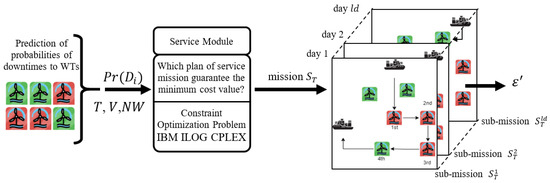
Figure 4.
Process of service planning under predictive maintenance.
The input data include parameters characterizing the type of mission adopted (period T), risk of downtime (), OWF network parameters (number and location of WTs), fleet parameters (V, and others), and service team parameters (). At the first stage, a subset of WTs to be serviced for a given day q is determined. At the next stage, a service mission, , is determined. For this purpose, the Constraint Optimization Problem is formulated and implemented in a declarative programming environment (e.g., IBM ILOG CPLEX). Its admissible solutions, , including the routes of vessel fleet and service team schedules, form the service mission: ). The mission designated in this way is assessed in terms of the number of prevented downtime events, i.e., maintenance efficiency .
The most significant advantage of using this model is the ability to freely change the configuration of the parameters of the searched mission, resulting from the declarative nature of the model. Depending on the assumptions made, the dispatcher can determine both the form of decision variables and the constraints binding them without changing the algorithm responsible for searching for a solution. The ability to take additional constraints into account in a friendly manner is particularly important in the considered application area where dispatchers operate in a constantly changing environment (weather, state of sea, vessel and crew changes, etc.).
5. Formulation of Efficiency
5.1. Prediction Efficiency—Discrete Prediction Outcomes
In this section, we explore the different methods for the formulation of the efficiency metrics. At first, this is based on the discrete prediction outcomes, as the simplest and most straightforward approach. After this is formulated, the ways in which this method is not satisfactory are then discussed. A better approach is presented afterward, built on continuous evaluation metrics.
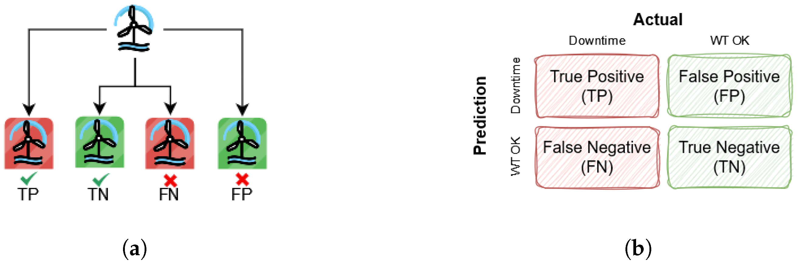
Traditionally, when analyzing the performance of classification models, a fixed threshold is assumed for deciding the class labels. For specific cases, the threshold can be manually adjusted; however, for most analysis tasks, a threshold of is used. Concerning the predictions of this paper, this means that a prediction score of and below results in a prediction of WT OK, and a prediction score of and above results in a prediction of downtime event. This simplifies the analysis to the prediction outcomes of True Positives (TP), True Negatives (TN), False Positives (FP), and False Negatives (FN). This is also commonly known as a confusion matrix–see Figure 5.
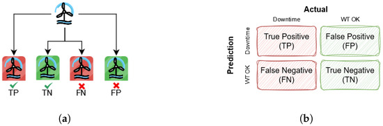
Figure 5.
These figures show the prediction outcomes. Note that the red color represents a WT with imminent downtime event which is the positive event: (a) Discrete mapping of prediction outcomes; (b) a confusion matrix of prediction outcomes.
In the case of many predictions, e.g., for a WF considered for maintenance, the total number of prediction outcomes are summed up across all predictions, such that , , , and denote the total number of prediction outcomes. Given this, can be formulated as one subtracted by the ratio of correctly predicted downtime events to total amount of downtime events (also called the recall/sensitivity ); see Equation (7).
This approach would be acceptable in the model training phase to compare different model performances, as only the binary outcomes are sought to be as accurate as possible. However, when used in predictive maintenance, this is not ideal, as information is lost when collapsing to the discrete outcomes. Given two WTs predicted with imminent downtime, these would be indistinguishable without the exact prediction scores, which could help prioritize which WT to service first. Additionally, this formulation of does not consider model uncertainty but only discrete classifications. In the real case of prediction, when , classifying the WT prediction score into one of the prediction outcomes of TP, TN, FP, FN is not possible as the true labels are unknown. The prediction score could instead be partially classified (with a specific level of membership) for each of them. For this purpose, more complex models that take into account non-discrete prediction outcomes are required.
To mitigate these above-described issues, the following efficiency requirements are stated, which when adhered to will help develop a more meaningful efficiency metric.
5.2. Efficiency Requirements
The above-described limitations have led us to identify the following three requirements for the efficiency metrics:
- Requirement 1—Must preserve the continuous nature of the prediction scores.
- Requirement 2—Must reflect the model uncertainty for each prediction outcome.
- Requirement 3—Must be useful for estimating potential outcomes in cases where the true labels are unknown.
Requirement 1 is necessary, as dealing with limited resources requires some decisions to be made. To choose between two WTs with a high risk of downtime events, we require that the continuous prediction scores are preserved such that this information can be used to decide on the optimal maintenance plan, i.e., a WT with a prediction score of is more reasonable to maintain than a WT with a prediction score of . Additionally, a prediction score of is valuable to prioritize over a prediction score of , even though both would be classified as having no imminent downtime events. The importance of this was explored in [12], where the prediction scores are used to evaluate the possible impacts of the downtime events.
Requirement 2 ensures that each prediction score is evaluated across all prediction outcomes to obtain a more accurate picture of the model uncertainty. Given a prediction score of , there is also the opposite event prediction of , which must be evaluated based on the prediction outcomes as well. This means that all prediction scores are partly correct and incorrect, and must be evaluated rather on how close the prediction score was to the true label. In the situation where the prediction score is exactly 0 but a downtime event happens, this must be considered more uncertain than if the prediction score was .
Where the two first requirements are focused on the evaluation of the model, Requirement 3 is based on the maintenance use cases. When planning a service mission, the true labels will be unknown, and the prediction outcomes cannot be evaluated. In this case, based on the evaluation of the model compared with historical data, expected prediction outcomes can be calculated instead of using the known model uncertainty. This will facilitate a cost–benefit analysis of the implementation of the predictive maintenance on specific cases.
5.3. Prediction Efficiency—Continuous Prediction Scores
To create an efficiency metric that follows the above-described requirements, a prediction membership score is necessary for each prediction outcome. These membership scores will intuitively demonstrate a measure of how well any prediction score fits each outcome, thereby describing the model uncertainty. After normalization of the membership scores, they can be used to evaluate for specific cases with no knowledge of the true labels.
The below distance function Equation (8), allows the approach to satisfy Requirement 1 by measuring the absolute gap between a prediction score and the correct label, instead of using categorical outcomes. This does not regard whether the true labels are 1 or 0 but simply finds how close a prediction score is to the true label. This allows us to not only assess but also allows for to be included in further analysis.
It follows that is bounded by 0 and 1. A larger means that the prediction is further from the correct label while a smaller indicates predictions close to the correct label. Note that all predictions with would be classified as a correct prediction in the case of binary classification.
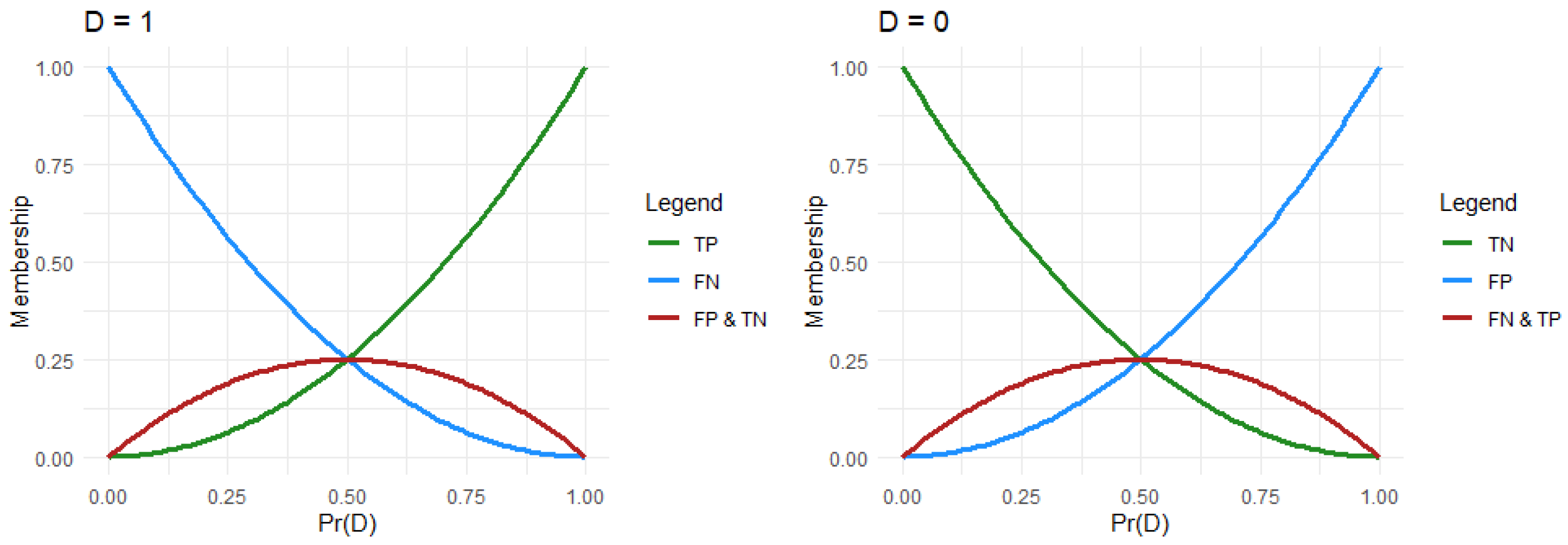
A membership function for each prediction outcome is then calculated; see Equations (9)–(12). These functions will satisfy Requirement 2, as they evaluate each of the four prediction outcomes and then a weighted distance for both the prediction scores, as well as the prediction scores of the opposite event. The shape of these membership functions is presented in Figure 6, and it can be seen how the membership functions distribute the partial membership based on the prediction score.
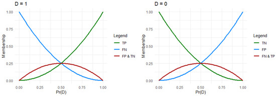
Figure 6.
The shape of the membership functions. On the left is the case with and on the right is the case with .
As an example, if and , then , which is evaluated with membership scores (according to Equations (9)–(12)) belonging to the TP class with level , to classes FP with level , FN with level , and TN with level . From this, it can be observed that even though the prediction score would evaluated to the true label in the discrete case, this approach will penalize the uncertain prediction scores in the membership evaluation.
For a given model, the above membership functions may be evaluated for a series of predictions with known labels in the validation process. Averaging the membership distribution across this validation process, the membership scores are found for that specific model; see Equations (13)–(16). These membership scores are model-specific scores of how to non-categorically assign the prediction scores to each of the prediction outcomes.
A high and score represents that the model is reliable in the prediction scores, and by looking at the membership scores individually, we are also able to understand in which prediction labels the model struggles the most. High and are understood, as we can expect the model to make mistakes in the associated prediction outcomes. These membership scores are a representation of the overall expected model performance and can be used to estimate the distribution of outcomes given a series of predictions without known labels.
In the last step, and to fulfill Requirement 3, a normalization of the above membership scores is necessary, which is notated as , etc. They are normalized in pairs such that and . If not normalized, the prediction score membership among the prediction outcomes will not sum up one. In a scenario with unknown labels, by instead multiplying the prediction scores with the normalized membership scores, an expected outcome of the prediction can be evaluated, which we note with the expected () notation; see Equations (17) and (18). Because of the normalization, Equation (19) holds for any , and this is specifically what satisfies Requirement 3.
Based on the normalized membership scores, a new formulation of the efficiency metric can be made; see Equation (20), which has been derived with a method that satisfies all the listed requirements.
A simple numerical example that presents this process can be found in the below tables. Table 1 shows the validation process, which derives the membership scores of the model, and Table 2 uses these membership scores to estimate for a simple case where the event labels are unknown. In this case, the prediction efficiency is , which can be understood as the expected performance of the model, e.g., it will correctly predict 85% of the downtime events.

Table 1.
The process of calculating the normalized membership scores.
Table 2.
The expected outcome of a series of downtime predictions where the true label is unknown.
5.4. Maintenance Efficiency
As the maintenance efficiency depends on the specific service mission, this metric can never rely on the true event labels. Instead, to find the maintenance efficiency, , the expected outcome based on the prediction model membership scores is used again. To differentiate between the WTs that are serviced and those that are not, we now introduce the notation. The difference between and is simply that only considers the WTs that are serviced (see Table 3) and does not evaluate the WTs that are not serviced. Based on this notation, can now be formulated as in Equation (21). Contrary to where only the true positives were relevant, this time the false negatives are also included in the numerator, as this represents downtime events not predicted but still experienced. Also note that the denominator uses the former expected outcomes and is not limited to the maintained WTs. This is necessary as we wish to evaluate the prevention rate for the whole OWF.
Table 3.
Following from Table 2 in the case of maintained WTs such that only WTs selected for maintenance are included.
To follow the example from the previous section, Table 3 shows the service outcome with a strategy of simply maintaining the WTs with the highest prediction scores and assuming the service capability of three maintained WTs per day. This table now presents the resulting prevention of downtime events on the first day of maintenance. The second day of maintenance is disregarded in this example, as all WTs will be maintained on the second day and all downtime events are prevented. This results in . A more involved example is explored in Section 7.
In the above example, there is a decrease in the maintenance efficiency compared with prediction efficiency because of the limited capabilities of the service mission. One WT obtained a prediction score of but without maintenance being planned on this day, as other WTs took priority. This will decrease the overall service efficiency, as it is more than likely that this would result in a downtime event.
Comparing these efficiencies can yield interesting knowledge on the predictive maintenance strategy as a whole. More generally, we would like to note the following possible conclusions that can be made.
- 1.
- —This would indicate that the service resources are the operational bottleneck. There is potential in increasing service resources given that the interventions are sufficiently cost-efficient.
- 2.
- —This would indicate that the prediction model is low-performing and does not add value. If this is not the case, then service capabilities are so high that the maintenance is performing well disregarding and negating the impacts of predictive maintenance.
- 3.
- —In the case that the efficiency metrics are low, this indicates a well-performing predictive maintenance strategy. In the case that both are high, this indicates the independent bad performance of the predictive model and of the service mission.
A more involved case study with a maintenance mission spanning several days and based on an actual case is considered in the next section. This deeper case study will also include the cost models such that not only the efficiencies are described but also the marginal changes in overall costs.
6. Case Study
In the following sections, the case study is presented, which is based on a practical scenario. The parameters of the case are reflective of actual service work undertaken by service providers in the field. The service mission will be evaluated by , , and total costs, which are then compared between preventive and predictive maintenance. The only difference between these two strategies is the information on downtime event risks given by the prediction model and the inclusion of this information in the prioritization of WT selection.
6.1. Case Parameters
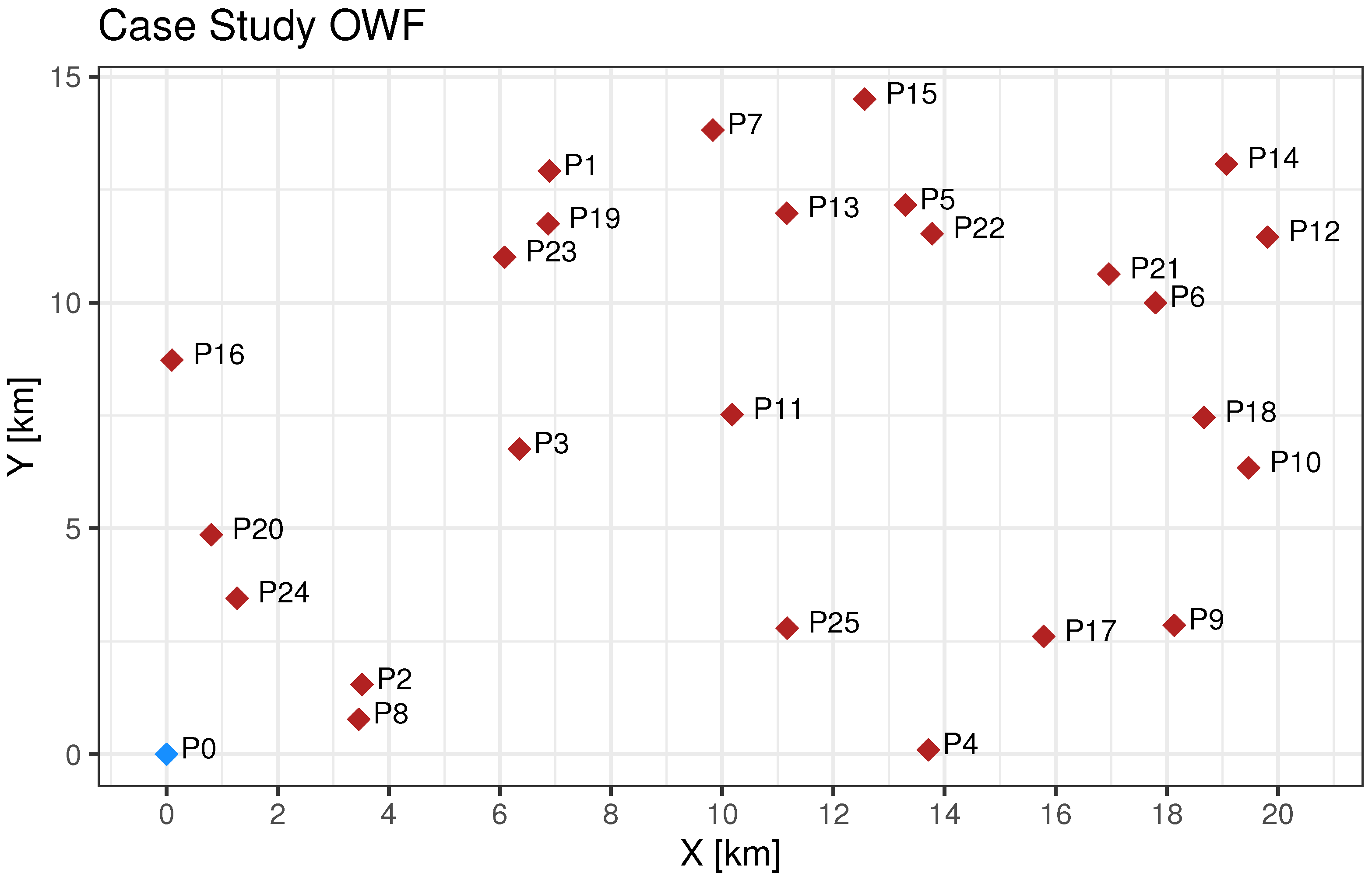
The case parameters are highly specific for this scenario and must be reconsidered for any other case. The service mission involves an annual service of 25 WTs, each of which must be serviced by a team delivered and picked up by a service vessel under all assumptions made in Section 5.2. The number of vessels, service teams, and operational costs are presented in Table 4, and the coordinates of the OWF can be seen in Figure 7. Point is the dock, which is close to the OWF, which indicates that this is a nearshore OWF. For OWFs situated further from land, the initial travel times should be considered as well and reduce the total number of WTs serviced per day. The purpose of this service mission is to visit every WT, which is expected to last for three days with the available resources. The OWF consists of 3.6 MW WTs and is receiving subsidized energy prices at EUR 168 per MWh. The wind is assumed to be ideal for wind energy production during the days of service with a wind factor of 0.9. Lastly, by examination of historical data on the OWF, the mean duration of downtime events was found to be 3.5 h.
Table 4.
Costs concerning the maintenance resources.
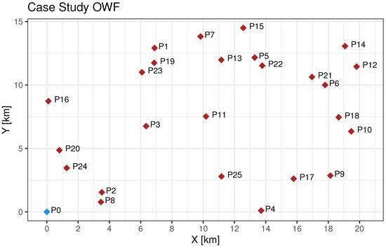
Figure 7.
Considered WTs for the case study. Red points are WTs, and the blue point is the dock. The irregular positions are because this is a subset of a full OWF selected for annual service.
6.2. Predictive Maintenance
The predictive model has provided prediction scores for imminent downtime events for the considered WTs for each of the three days. These prediction scores can be seen in Table 5. Along with this, during the validation process, the membership scores are found and can be seen in Table 6, which are calculated following Equations (13)–(16). These distribution scores are fairly well performing, as the model has proven in the validation process to be quite effective.
Table 5.
Prediction scores for the three days considered for the service mission.
Table 6.
Membership scores of the prediction model used in the case study.
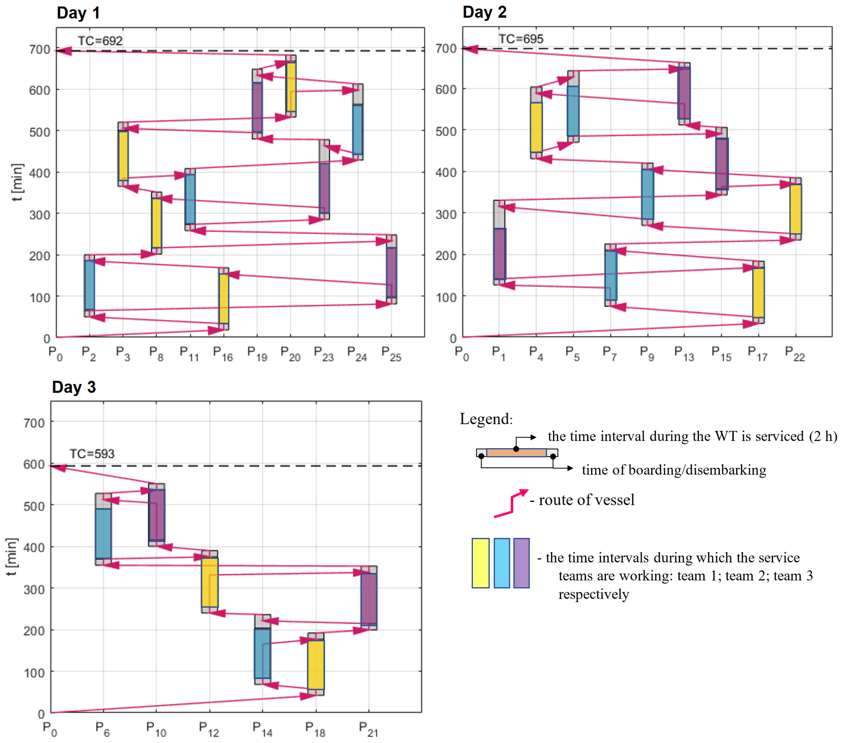
The WT selection strategy, given this information, is to select the WTs with the highest prediction scores per day of service. This will hopefully maximize the number of downtime events prevented. This results in the service plan presented in Table 7. For this selection, the daily travel plan is based on minimizing the travel time, which results in the daily vessel schedule seen in Figure 8. This service plan results in fewer WTs serviced in the first days as the WTs are further apart; however, all WTs are still able to be serviced within the three days.
Table 7.
Service plan of WTs for service under predictive maintenance.
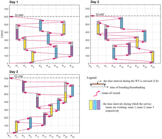
Figure 8.
The service schedule for each day of the service mission under predictive maintenance.
Based on the membership scores, the expected number of downtime events is found for each day. Additionally, the correctly predicted downtime events are also evaluated, and then by Equation (20), we obtain . Given the service plan, lastly the cumulative prevented downtime events are found, which by Equation (21) results in . This is all presented in Table 8.
Table 8.
Overview of the predicted and prevented number of downtime events in addition to and under predictive maintenance.
6.3. Preventive Maintenance
Under preventive maintenance, the strategy of WT selection for each day of service maximizes the number of WTs serviced per day. This results in the service plan presented in Table 9. Once again, the daily travel plan is based on minimizing the travel time between the selected WTs, which results in the daily vessel schedule seen in Figure 9. It is clear that the strategy of servicing as many WTs as possible as early as possible will result in more WTs serviced on day one, and the WTs located further from the dock will be serviced last.
Table 9.
Service plan of WTs for service under preventive maintenance.
Figure 9.
The service schedule for each day of the service mission under preventive maintenance.
As there is no prediction model to provide risk scores of downtime events, cannot be evaluated under preventive maintenance. The expected number of downtime events will still be based on the model prediction scores, as it is necessary to compare the impacts of maintenance given the same assumed number of downtimes. From the service plan, the cumulative prevented downtime events are found, which results in . This is presented in Table 10. This is a fairly good result, achieved as preventive maintenance optimizes the number of WTs serviced and hence prevents a high number of downtime events by pure chance.
Table 10.
The expected downtime prevention rate and under preventive maintenance.
With the above results, we can now safely assume that predictive maintenance will in this scenario be more efficient concerning downtime events and is expected to prevent more downtime events compared with preventive maintenance. What is left to fully understand is if this decrease in downtime events will lead to overall fewer costs, as it requires a slightly more complex service schedule.
6.4. Cost Analysis
The service costs are provided by the declarative model solution and consist of fixed daily costs for the vessel and team in addition to the spent fuel. As there are no changes in the number of days used for the service mission regardless of maintenance strategy, the fixed costs do not change in this case study. If this had been the case, the increased service costs would incrementally increase markedly per extra day of service. Revenue and costs of downtime follow Equations (2) and (3) by using the parameters presented at the beginning of this section, and the total profits over the three-day period is summarized by Equation (6). The cost of predictive services is difficult to assess under a real scenario like this, as this will consist of many immeasurable components. As the total predictive modeling development costs can be distributed among all other use cases and over the many annual services that must be performed over an OWF lifetime, it is safe to assume that the fraction to include in this annual case study is fairly small, and EUR 500 is used.
All costs for predictive maintenance can be found in Table 11, while costs for preventive maintenance are found in Table 12. By comparing all numbers in the two above tables and considering as well, we arrive at a total overall cost saving of EUR by implementing predictive maintenance. The negative profit numbers simply reflect that the performed service mission and downtime events overall cost more than the potential revenue during this three-day mission.
Table 11.
Potential revenue and costs for the service mission under predictive maintenance with .
Table 12.
Potential revenue and costs for the service mission under preventive maintenance with .
If the OWF was not subsidized, the overall solutions provided by predictive maintenance would indeed be more expensive overall as the cost of downtime events becomes cheaper. This shows well that predictive maintenance is not inherently cost-efficient in all scenarios when comparing the already existing maintenance strategies, as the marginal impact is limited by the efficiency of existing maintenance. The cost of a downtime event must be much more expensive to warrant the increased complexity of service.
In the above case, there are limited short-term advantages to implementation of the predictive maintenance, and a decision taker might well decide to not change a functional system for such low gain. However, this decision maker might still be interested in the potential of predictive maintenance, as this potential could provide an incentive to further improve the predictive model such that it becomes more viable to use and will show the upper limit of savings that are possible to achieve with predictive maintenance.
For this evaluation, the maintenance costs are evaluated for the perfect model, meaning an unrealistic model with . This means that the model prediction scores will exactly mirror the true labels, which results in the membership scores from Table 13. The prediction scores of such a perfect model will only output the exact discrete labels, as it makes no mistakes. The service mission schedule from predictive maintenance in Table 7 is used.
Table 13.
Membership scores of the prediction model if the model is a perfect predictor.
Thus, discretizing the prediction scores and counting the total, predicted, and prevented downtime events as previously, we obtain the results of Table 14, where we can see that only a single downtime event was not prevented. This results in the overall costs seen in Table 15. The only change compared with the original cost calculations for predictive maintenance is the decrease in costs of downtime, which is significantly lower. The difference is EUR , which is the further potential benefit of improving the predictive modeling for this specific service mission. By weighing this potential against the costs of further predictive improvements, a decision about making predictive maintenance viable or completely abandoning predictive maintenance for this use case can be supported.
Table 14.
Overview of the predicted and prevented number of downtime events in addition to and with a perfect prediction model.
Table 15.
Potential revenue and costs for the service mission with a perfect prediction model.
7. Discussion
The key takeaway from the case above is that the minimum cost maintenance solution is not decisively in favor of predictive maintenance. If the energy price was not subsidized, the cost–benefit analysis would have clearly been in favor of preventive maintenance. This outcome indicates how important the price of service and the price of downtime events is. Even in other scenarios where the technical failure could be much more expensive than simply lost production, there will be an equal increase in the service costs. Predictive maintenance then requires that the underlying predictive model is performing well, as few false positive predictions are enough to negate the benefits.
Although the point made above points to the fact that predictive maintenance does not always carry significant benefits in the short term, this should be weighed against the long-term benefits. Missing from the analysis methodology of this paper is the impacts of predictive maintenance in the long term, where the compounding effects of optimized asset conditions might provide more significant benefits. Different analysis tools are necessary to capture this long-term perspective, but this is generally more available in the literature.
The methodology is not limited to the exact scenario of the case study where the difference between preventive and predictive maintenance is evaluated. In the case study, the resources available and the WT selection strategy were fixed, but if this was not the case, the methodology could similarly be utilized to compare the impacts of additional maintenance resources or slightly different selection strategies. For example, the predictive maintenance case presented in this paper used a selection strategy of simply prioritizing the highest risk WTs. By exploring other options of maintenance prioritization that involves a more holistic service perspective, further cost improvements might be available and might be identified with the presented evaluation methodology.
We also have to note that the minimization of the overall cost of service is not similar to the minimization of . To find the optimal maintenance strategy, strictly focusing on the minimization of will result in overall higher costs, as the costs of service will increase disproportionately for the last few percentage points of efficiency. Exploring the optimal level of with regards to overall cost and which parameters influence it significantly is itself a separate research topic and is explored in [58].
8. Conclusions
Addressing the knowledge gap within short-term implications of predictive maintenance, the main contribution of this work is thus a methodology to perform an evaluation of the specific predictive maintenance operation for OWFs. This methodology was facilitated by uncertainty analysis of the predictive model itself and the expected efficiency of service planning performed with risk information of the predictive model.
The validation of this methodology was made by applying it to an industry-relevant case study. This found estimates of the overall short-term impacts of predictive maintenance, which resulted in fairly low improvements of of the overall costs compared with preventive maintenance. This shows that the implementation of such specific predictive maintenance services might provide limited short-term benefits mainly due to the effectiveness of the existing preventive maintenance.
We believe that the methodology shown in this paper will definitely support better assessments of predictive maintenance strategies. However, for any specific case where this methodology is used, all costs concerning maintenance, downtime/failure, and predictive modeling must be carefully formulated to fit the case as the conclusions that are obtained are much influenced by these costs. Some components of the method, like the distance measure and the membership function, have alternatives and could as well be fine-tuned to the specific case. If successfully implemented widely for OWFs, this will result in a better overall understanding of short-term predictive maintenance impacts, assist decision-makers in finding optimal maintenance solutions, and complement the existing literature on the long-term benefits of predictive maintenance.
Further Work
Further work should facilitate commercial use and explore limiting factors of predictive maintenance. The largest identified limitation is the performance of the predictive maintenance. As there are costs connected to the switch to predictive maintenance, as the model providing the predictions decreases in performance, the benefits of predictive maintenance will decrease as well. The numerical study of this paper proved limited upside to the implementation of predictive maintenance, and an only slightly worse-performing model would see the two maintenance strategies performing at equal levels. Finding the exact model performance where predictive maintenance shifts to being cost-effective is itself a very useful research objective.
To gain commercial relevance, a large number of use cases can be revealed by reactive maintenance as well. One of the main points of this paper is that predictive maintenance will be built upon existing maintenance; however, only application upon preventive maintenance was explored. In the case of reactive maintenance, new cost formulations must be made for the different scenarios concerning these maintenance operations, and the case of false positive predictions especially will incur significant costs, as maintenance will be performed unnecessarily. The membership distribution scores used to estimate the prediction outcomes from this paper could be utilized for the expected outcomes, just as is presented for preventive maintenance in this paper. By formulation of the additional costs and savings related to reactive maintenance, this methodology is readily available for this improvement, which would make the approach more broadly applicable to different maintenance scenarios.
A major advantage of this methodology is that it is readily applicable to many different maintenance scenarios, given that the costs are readily available. When dealing with any system of preventive/predictive maintenance, the presented approach can evaluate the efficiency regardless of the scenario considered. In this paper, the maintenance of OWFs was explored through annual service missions; however, many other maintenance operations can be improved with predictive modeling and can in similar ways be evaluated. This applicability is not limited by wind energy as well, as any industrial assets undergoing similar preventive maintenance or being considered for predictive maintenance can be evaluated with the same system. What must be adjusted specifically for the scenario considered are the cost metrics. The exact cost–benefit analysis is highly dependent on the situation and scenario and must be formulated independently, in addition to how the efficiency metrics will impact the cost–benefit analysis.
Author Contributions
Conceptualization, G.B. and Z.B.; Methodology, R.D.F., G.B. and G.R.; Software, R.D.F. and G.R.; Validation, R.D.F.; Formal analysis, G.B.; Investigation, G.R.; Data curation, R.D.F.; Writing—original draft, R.D.F.; Writing—review & editing, R.D.F., G.B., Z.B. and P.N.; Visualization, R.D.F. and G.B.; Supervision, G.B., Z.B. and P.N.; Project administration, Z.B. and P.N. All authors have read and agreed to the published version of the manuscript.
Funding
This research received no external funding.
Data Availability Statement
The data presented in this study are available on request from the corresponding author in anonymized format due to strict legal rules against sharing of data.
Conflicts of Interest
The authors declare no conflicts of interest.
References
- Lazard. 2023 Levelized Cost Of Energy+ | Lazard; Technical report; Lazard: San Francisco, CA, USA, 2023. [Google Scholar]
- Taylor, M.; Ralon, P.; Al-Zoghoul, S.; Epp, B.; Jochum, M. Renewable Power Generation Costs 2020; IREA: Sedalia, CO, USA, 2021; pp. 1–180. [Google Scholar]
- Stehly, T.; Duffy, P.; Mulas Hernando, D. 2022 Cost of Wind Energy Review; Technical report; NREL: Golden, CO, USA, 2023. [Google Scholar]
- Fox, H.; Pillai, A.C.; Friedrich, D.; Collu, M.; Dawood, T.; Johanning, L. A Review of Predictive and Prescriptive Offshore Wind Farm Operation and Maintenance. Energies 2022, 15, 504. [Google Scholar] [CrossRef]
- Khan, M.; Ahmad, A.; Sobieczky, F.; Pichler, M.; Moser, B.A.; Bukovsky, I. A Systematic Mapping Study of Predictive Maintenance in SMEs. IEEE Access 2022, 10, 88738–88749. [Google Scholar] [CrossRef]
- Qasim, M.; Khan, M.; Mehmood, W.; Sobieczky, F.; Pichler, M.; Moser, B. A Comparative Analysis of Anomaly Detection Methods for Predictive Maintenance in SME. In Communications in Computer and Information Science; Springer: Cham, Switzerland, 2022; Volume 1633. [Google Scholar]
- Butte, S.; Prashanth, A.R.; Patil, S. Machine Learning Based Predictive Maintenance Strategy: A Super Learning Approach with Deep Neural Networks. In Proceedings of the 2018 IEEE Workshop on Microelectronics and Electron Devices, WMED 2018, Boise, ID, USA, 20 April 2018. [Google Scholar]
- Cevasco, D.; Koukoura, S.; Kolios, A.J. Reliability, availability, maintainability data review for the identification of trends in offshore wind energy applications. Renew. Sustain. Energy Rev. 2021, 136, 110414. [Google Scholar] [CrossRef]
- Kaldellis, J.K.; Zafirakis, D. The influence of technical availability on the energy performance of wind farms: Overview of critical factors and development of a proxy prediction model. J. Wind Eng. Ind. Aerodyn. 2013, 115, 65–81. [Google Scholar] [CrossRef]
- Turnbull, A.; Carroll, J. Cost benefit of implementing advanced monitoring and predictive maintenance strategies for offshore wind farms. Energies 2021, 14, 4922. [Google Scholar] [CrossRef]
- Banaszak, Z.; Radzki, G.; Nielsen, I.; Frederiksen, R.; Bocewicz, G. Proactive Mission Planning of Unmanned Aerial Vehicle Fleets Used in Offshore Wind Farm Maintenance. Appl. Sci. 2023, 13, 8449. [Google Scholar] [CrossRef]
- Bocewicz, G.; Frederiksen, R.D.; Nielsen, P.; Banaszak, Z. Integrated preventive–proactive–reactive offshore wind farms maintenance planning. Ann. Oper. Res. 2024. [Google Scholar] [CrossRef]
- Lemming, J.K.; Morthorst, P.E.; Clausen, N.E.; Jensen, P. General rights Contribution to the Chapter on Wind Power. In Energy Technology Perspectives 2008; IEA: Paris, France, 2009. [Google Scholar]
- Beiter, P.; Cooperman, A.; Lantz, E.; Stehly, T.; Shields, M.; Wiser, R.; Telsnig, T.; Kitzing, L.; Berkhout, V.; Kikuchi, Y. Wind power costs driven by innovation and experience with further reductions on the horizon. Wiley Interdiscip. Rev. Energy Environ. 2021, 10, e398. [Google Scholar] [CrossRef]
- Wiser, R.; Jenni, K.; Seel, J.; Baker, E.; Hand, M.; Lantz, E.; Smith, A. Forecasting Wind Energy Costs & Cost Drivers. IEA Wind Task 2016, 1, 1–6. [Google Scholar]
- Enevoldsen, P.; Xydis, G. Examining the trends of 35 years growth of key wind turbine components. Energy Sustain. Dev. 2019, 50, 18–26. [Google Scholar] [CrossRef]
- Voormolen, J.A.; Junginger, H.M.; van Sark, W. Unravelling historical cost developments of offshore wind energy in Europe. Energy Policy 2016, 88, 435–444. [Google Scholar] [CrossRef]
- Blanco, M.I. The economics of wind energy. Renew. Sustain. Energy Rev. 2009, 13, 1372–1382. [Google Scholar] [CrossRef]
- Sun, L.; Yin, J.; Bilal, A.R. Green financing and wind power energy generation: Empirical insights from China. Renew. Energy 2023, 206, 820–827. [Google Scholar] [CrossRef]
- Gatzert, N.; Kosub, T. Risks and risk management of renewable energy projects: The case of onshore and offshore wind parks. Renew. Sustain. Energy Rev. 2016, 60, 982–998. [Google Scholar] [CrossRef]
- Đukan, M.; Kitzing, L. The impact of auctions on financing conditions and cost of capital for wind energy projects. Energy Policy 2021, 152, e112197. [Google Scholar] [CrossRef]
- Ziegler, L.; Gonzalez, E.; Rubert, T.; Smolka, U.; Melero, J.J. Lifetime extension of onshore wind turbines: A review covering Germany, Spain, Denmark, and the UK. Renew. Sustain. Energy Rev. 2018, 82, 1261–1271. [Google Scholar] [CrossRef]
- Chiesura, G.; Stecher, H.; Jensen, J.P. Blade materials selection influence on sustainability: A case study through LCA. IOP Conf. Ser. Mater. Sci. Eng. 2020, 942, 12011. [Google Scholar] [CrossRef]
- Demuytere, C.; Vanderveken, I.; Thomassen, G.; Godoy León, M.F.; De Luca Peña, L.V.; Blommaert, C.; Vermeir, J.; Dewulf, J. Prospective material flow analysis of the end-of-life decommissioning: Case study of a North Sea offshore wind farm. Resour. Conserv. Recycl. 2024, 200, 107283. [Google Scholar] [CrossRef]
- Li, D.; Zhang, Z.; Zhou, X.; Zhang, Z.; Yang, X. Cross-wind dynamic response of concrete-filled double-skin wind turbine towers: Theoretical modelling and experimental investigation. J. Vib. Control 2023, 1, 1–3. [Google Scholar]
- Junginger, M.; Louwen, A. Technological Learning in the Transition to a Low-Carbon Energy System: Conceptual Issues, Empirical Findings, and Use in Energy Modeling; Academic Press: Cambridge, MA, USA, 2019; pp. 321–326. [Google Scholar]
- Lu, Y.; Sun, L.; Xue, Y. Research on a comprehensive maintenance optimization strategy for an offshore wind farm. Energies 2021, 14, 965. [Google Scholar] [CrossRef]
- Yan, R.; Dunnett, S. Improving the strategy of maintaining offshore wind turbines through petri net modelling. Appl. Sci. 2021, 11, 574. [Google Scholar] [CrossRef]
- Santhakumar, S.; Heuberger-Austin, C.; Meerman, H.; Faaij, A. Technological learning potential of offshore wind technology and underlying cost drivers (Under Review). Sustain. Energy Technol. Assess. 2021, 60, e103545. [Google Scholar]
- Gonzalez, E.; Nanos, E.M.; Seyr, H.; Valldecabres, L.; Yürüşen, N.Y.; Smolka, U.; Muskulus, M.; Melero, J.J. Key Performance Indicators for Wind Farm Operation and Maintenance. Energy Procedia 2017, 137, 559–570. [Google Scholar] [CrossRef]
- Hofmann, M. A Review of Decision Support Models for Offshore Wind Farms with an Emphasis on Operation and Maintenance Strategies. Wind Eng. 2011, 35, 1–15. [Google Scholar] [CrossRef]
- Costa, Á.M.; Orosa, J.A.; Vergara, D.; Fernández-Arias, P. New Tendencies in Wind Energy Operation and Maintenance. Appl. Sci. 2021, 11, 1386. [Google Scholar] [CrossRef]
- Shihavuddin, A.S.; Chen, X.; Fedorov, V.; Christensen, A.N.; Riis, N.A.B.; Branner, K.; Dahl, A.B.; Paulsen, R.R. Wind turbine surface damage detection by deep learning aided drone inspection analysis. Energies 2019, 12, 676. [Google Scholar] [CrossRef]
- Huang, X.; Wang, G. Saving Energy and High-Efficient Inspection to Offshore Wind Farm by the Comprehensive-Assisted Drone. Int. J. Energy Res. 2024, 2024, 6209170. [Google Scholar] [CrossRef]
- Shafiee, M.; Zhou, Z.; Mei, L.; Dinmohammadi, F.; Karama, J.; Flynn, D. Unmanned aerial drones for inspection of offshore wind turbines: A mission-critical failure analysis. Robotics 2021, 10, 26. [Google Scholar] [CrossRef]
- Eisenberg, D.; Laustsen, S.; Stege, J. Wind turbine blade coating leading edge rain erosion model: Development and validation. Wind Energy 2018, 21, 942–951. [Google Scholar] [CrossRef]
- Lau, B.C.P.; Ma, E.W.M.; Pecht, M. Review of offshore wind turbine failures and fault prognostic methods. In Proceedings of the IEEE 2012 Prognostics and System Health Management Conference, PHM-2012, Minneapolis, MN, USA, 23–27 September 2012. [Google Scholar]
- Gao, Z.; Liu, X. An overview on fault diagnosis, prognosis and resilient control for wind turbine systems. Processes 2021, 9, 300. [Google Scholar] [CrossRef]
- Yeter, B.; Garbatov, Y.; Guedes Soares, C. Risk-based maintenance planning of offshore wind turbine farms. Reliab. Eng. Syst. Saf. 2020, 202, 107062. [Google Scholar] [CrossRef]
- Sinha, Y.; Steel, J.A. A progressive study into offshore wind farm maintenance optimisation using risk based failure analysis. Renew. Sustain. Energy Rev. 2015, 42, 735–742. [Google Scholar] [CrossRef]
- Shafiee, M. Maintenance logistics organization for offshore wind energy: Current progress and future perspectives. Renew. Energy 2015, 77, 182–193. [Google Scholar] [CrossRef]
- Poulsen, T.; Hasager, C.B. How expensive is expensive enough? Opportunities for cost reductions in offshoreWind energy logistics. Energies 2016, 9, 437. [Google Scholar] [CrossRef]
- Jin, T.; Tian, Z.; Huerta, M.; Piechota, J. Coordinating maintenance with spares logistics to minimize levelized cost of wind energy. In Proceedings of the 2012 International Conference on Quality, Reliability, Risk, Maintenance, and Safety Engineering, ICQR2MSE 2012, Chengdu, China, 15–18 June 2012. [Google Scholar]
- Cai, J.; Liu, Y.; Zhang, T. Preventive maintenance routing and scheduling for offshore wind farms based on multi-objective optimization*. In Proceedings of the 2022 First International Conference on Cyber-Energy Systems and Intelligent Energy (ICCSIE), Shenyang, China, 14–15 January 2023; pp. 1–6. [Google Scholar]
- Elusakin, T.; Shafiee, M.; Adedipe, T.; Dinmohammadi, F. A stochastic petri net model for o&m planning of floating offshore wind turbines. Energies 2021, 14, 1134. [Google Scholar] [CrossRef]
- Liu, X.; Chen, Y.L.; Por, L.Y.; Ku, C.S. A Systematic Literature Review of Vehicle Routing Problems with Time Windows. Sustainability 2023, 15, 12004. [Google Scholar] [CrossRef]
- Irawan, C.A.; Ouelhadj, D.; Jones, D.; Stålhane, M.; Sperstad, I.B. Optimisation of maintenance routing and scheduling for offshore wind farms. Eur. J. Oper. Res. 2017, 256, 76–89. [Google Scholar] [CrossRef]
- Jonker, T. The Development of Maintenance Strategies of Offshore Wind Farm; Technical Report; Delft University of Technology: Delft, The Netherland, 2017. [Google Scholar]
- Sperstad, I.B.; McAuliffe, F.D.; Kolstad, M.; Sjømark, S. Investigating Key Decision Problems to Optimize the Operation and Maintenance Strategy of Offshore Wind Farms. Energy Procedia 2016, 94, 261–268. [Google Scholar] [CrossRef]
- Sperstad, I.B.; Stålhane, M.; Dinwoodie, I.; Endrerud, O.E.V.; Martin, R.; Warner, E. Testing the robustness of optimal access vessel fleet selection for operation and maintenance of offshore wind farms. Ocean Eng. 2017, 145, 334–343. [Google Scholar] [CrossRef]
- Graves, A.; Harman, K.; Wilkinson, M.; Walker, R. Understanding Availability Trends of Operating Wind Farms. AWEA WINDPOWER 2008. Available online: https://www.researchgate.net/publication/237566981_UNDERSTANDING_AVAILABILITY_TRENDS_OF_OPERATING_WIND_FARMS (accessed on 10 March 2024).
- Wang, X.; Zheng, Z.; Jiang, G.; He, Q.; Xie, P. Detecting Wind Turbine Blade Icing with a Multiscale Long Short-Term Memory Network. Energies 2022, 15, 2864. [Google Scholar] [CrossRef]
- Burmeister, N.; Frederiksen, R.D.; Hog, E.; Nielsen, P. Exploration of Production Data for Predictive Maintenance of Industrial Equipment: A Case Study. IEEE Access 2023, 11, 102025–102037. [Google Scholar] [CrossRef]
- Udo, W.; Muhammad, Y. Data-Driven Predictive Maintenance of Wind Turbine Based on SCADA Data. IEEE Access 2021, 9, 162370–162388. [Google Scholar] [CrossRef]
- Kusiak, A.; Li, W. The prediction and diagnosis of wind turbine faults. Renew. Energy 2011, 36, 16–23. [Google Scholar] [CrossRef]
- Schlechtingen, M.; Ferreira Santos, I. Comparative analysis of neural network and regression based condition monitoring approaches for wind turbine fault detection. Mech. Syst. Signal Process. 2011, 25, 1849–1875. [Google Scholar] [CrossRef]
- Kusiak, A.; Verma, A. A data-mining approach to monitoring wind turbines. IEEE Trans. Sustain. Energy 2012, 3, 150–157. [Google Scholar] [CrossRef]
- Frederiksen, R.D.; Bocewicz, G.; Nielsen, P.; Radzki, G.; Wójcik, R.; Banaszak, Z. Towards Efficiency: Declarative Modelling in Wind Farm Preventive Maintenance Strategies (In Print). In Proceedings of the 32nd International Conference on Information Systems Development, Gdańsk Metropolitan Area, Poland, 24–26 August 2024. [Google Scholar]

Disclaimer/Publisher’s Note: The statements, opinions and data contained in all publications are solely those of the individual author(s) and contributor(s) and not of MDPI and/or the editor(s). MDPI and/or the editor(s) disclaim responsibility for any injury to people or property resulting from any ideas, methods, instructions or products referred to in the content. |
© 2024 by the authors. Licensee MDPI, Basel, Switzerland. This article is an open access article distributed under the terms and conditions of the Creative Commons Attribution (CC BY) license (https://creativecommons.org/licenses/by/4.0/).