Article

An Intelligent Power Transformers Diagnostic System Based on Hierarchical Radial Basis Functions Improved by Linde Buzo Gray and Single-Layer Perceptron Algorithms

1
Electrical Engineering and Materials Laboratory, Higher School of Electrical and Energy Engineering, Oran 31000, Algeria
2
Intelligent Control and Electrical Power System, Djilali Liabes University of Sidi Bel Abbes, Sidi Bel Abbes 22000, Algeria
3
ESSA-Tlemcen, Ecole Supérieure en Sciences Appliquées de Tlemcen, ESSA-Tlemcen, BP 165 RP Bel Horizon, Tlemcen 13000, Algeria
4
Canada Research Chair, Tier 1, ViAHT, Department of Applied Sciences, University Québec, Chicoutimi, QC G7H 2B1, Canada
*
Author to whom correspondence should be addressed.
Energies 2024, 17(13), 3171; https://doi.org/10.3390/en17133171
Submission received: 16 May 2024 / Revised: 14 June 2024 / Accepted: 18 June 2024 / Published: 27 June 2024

Abstract

:
Transformers are fundamental and among the most expensive electrical devices in any power transmission and distribution system. Therefore, it is essential to implement powerful maintenance methods to monitor and predict their condition. Due to its many advantages—such as early detection, accurate diagnosis, cost reduction, and rapid response time—dissolved gas analysis (DGA) is regarded as one of the most effective ways to assess a transformer’s condition. In this contribution, we propose a new probabilistic hierarchical intelligent system consisting of five subnetworks of the radial basis functions (RBF) type. Indeed, hierarchical classification minimizes the complexity of the discrimination task by employing a divide-and-conquer strategy, effectively addressing the issue of unbalanced data (a significant disparity between the categories to be predicted). This approach contributes to a more precise and sophisticated diagnosis of transformers. The first subnetwork detects the presence or absence of defects, separating defective samples from healthy ones. The second subnetwork further classifies the defective samples into three categories: electrical, thermal, and cellulosic decomposition. The samples in these categories are then precisely assigned to their respective subcategories by the third, fourth, and fifth subnetworks. To optimize the hyperparameters of the five models, the Linde–Buzo–Gray algorithm is implemented to reduce the number of centers (radial functions) in each subnetwork. Subsequently, a single-layer perceptron is trained to determine the optimal synaptic weights, which connect the intermediate layer to the output layer. The results obtained with our proposed system surpass those achieved with another implemented alternative (a single RBF), with an average sensitivity percentage as high as 96.85%. This superiority is validated by a Student’s t-test, showing a significant difference greater than 5% (p-value < 0.001). These findings demonstrate and highlight the relevance of the proposed hierarchical configuration.

1. Introduction

Power transformers are primary electrical devices and play an essential role in an electrical power system. Their proper functioning is decisive in guaranteeing users a reliable, secure, high-quality electrical energy supply. Indeed, the transformers ensure an energy-efficient transformation with minimum losses and the ability to switch between the different network levels. Transformers also regulate the voltage in an electrical system and permanently maintain a constant and stable voltage. Transformers are essential from an electrical safety viewpoint; they make it possible to isolate electrical circuits and guarantee protection to users against electrical shocks [1,2,3,4,5]. However, transformers face cumulative thermal and electrical stresses that can cause various incipient failures. These can have a significant impact on their operation and lifespan. So, due to the transformer’s importance and their constant exposure to stresses, and given their high cost (their cost can reach up to 60% of the budget relating to all the equipment installed in the substations), it is necessary to maintain and regularly monitor them to guarantee their reliability and to prolong their life expectancy.
To date, different approaches are implemented to monitor power transformers immersed in oil, including electrical measurements, dielectric measurements, dissolved gas analysis (DGA), etc. Among these, the DGA approach is widely recognized as one of the most effective methods for assessing the electrical transformer’s condition. This method consists of detecting electrical and thermal incipient failures by analyzing the gases dissolved in the insulating oil.
Indeed, cumulative stresses generally lead to failures (overheating, dielectric, electrical, etc.). These faults cause the internal components to deteriorate. Such deterioration can be detected by the gaseous by-products dissolved in the transformer oil, which are combustible or not: methane ( C H 4 ), carbon dioxide ( C O ), ethylene ( C 2 H 4 ), ethane ( C 2 H 6 ), acetylene ( C 2 H 2 ) , hydrogen ( H 2 ), oxygen ( O 2 ), and nitrogen ( N 2 ). By nature, mineral oils consist of different hydrocarbon molecules. Each one contains carbon–carbon (C-C) and/or carbon–hydrogen (C-H) bonds. Thermal, electrical, and/or dielectric stress can break some of these bonds, leadings to free radicals ( H * ,   C H 3 * ,   C H 2 * ,   C H * and/or C * …etc.). These ions recombine to form gas molecules such as hydrogen ( H - H ), methane (CH3-H), ethane ( C H 3 - C H 3 ), ethylene ( C H 2 = C H 2 ), or acetylene ( C H C H ) [1,6]:
-
Low-energy faults promote a single-bond gas formation: H 2 for partial discharges (DP) and C 2 H 6 for low-energy thermal faults (T1);
-
Moderate-intensity failures, such as high-energy overheating (T2), include the formation of double-bond gases C 2 H 4 ;
-
Faults generated at temperatures above 1200 °C, such as low-energy electrical faults (LED) or high-energy electrical faults (HED), induce the recombination of gases with triple bonds, more precisely C 2 H 2 ;
-
A cellulose decomposition (CD) type of failure generally induces the reconstruction of two gases: C O ( C O ) and C O 2 ( O = C = O ).
The literature presents several ingenious studies concerning the assessment of the transformer’s health condition from DGA data, including traditional methods based on ratios and codes: Rogers codes (R-C) [7], Duval triangle (D-T) [8], Dornenburg (D-C) and IEC codes (IEC-C) [9], etc., and/or artificial intelligence (AI) methods [10,11,12,13,14,15,16,17,18,19]. However, the methods based on ratios and code interpretation have several limitations: the requirement of knowledge acquired beforehand for diagnosis validation, incomplete exploitation of different gases, inability to determine the incipient faults’ degree of seriousness (due to the code’s incompleteness), etc. To overcome these problems, researchers have suggested modifications to the traditional methods [10,11,20]. In spite of that, it is still difficult to propose a generalized mathematical rule that includes all possible cases. Therefore, the main challenge consists in developing techniques able to gather experiences through learnings and operations and then converting this knowledge into accurate decision rules that can adapt to any cases. AI learning and optimization techniques can be seen as a panacea to this challenge and constitute compelling alternatives to overcome the limitations of traditional methods.
In this context, several studies based on intelligent discrimination techniques have been proposed. The study [10] introduces multiple automated expert systems, including an architecture based on a multilayer perceptron (MLP) neural network trained with the Levenberg–Marquardt algorithm and optimized by the Bayesian regularization algorithm, an architecture based on k-nearest neighbors (KNN), and a third architecture based on a support vector machine (SVM) with radial basis, linear, and polynomial kernel functions. Study [12] describes the use of Dempster–Shafer (DS) evidence theory for the fusion of outputs from three probabilistic classifiers, namely SVM, relevance vector machine (RVM), and MLP. The authors in [13] present a comparative study of MLP performance based on several conventional parameter extraction techniques. Studies [14,15] introduce two original approaches based on the use of extreme learning machines (ELM). Xie and co-authors [16] propose the implementation of support vector regression (SVR) for power transformer diagnosis, following the elimination of redundant features using a step-by-step feature selection approach. For monitoring transformer health status, the authors in [17] recommend implementing an SVM optimized by the Krill Herd algorithm, while study [18] suggests using an SVM optimized by a genetic algorithm. The authors in [19] present an approach based on DS fusion, applied to the outputs of four direct probabilistic multi-class SVMs. Nevertheless, all these methods are not necessarily effective for power transformer diagnosis. Indeed, the transformer diagnosis from DGA data is a difficult problem in itself; the gas concentrations of the different categories show a significant correlation. In addition, the training data are not large enough, and the non-homogeneity between categories tends to affect the classifier performance (knowing that these performances are generally linked to statistical concerns).
To define the most appropriate classification methods, the researchers carried out many comparative studies [10,12] and deduced the superiority of SVM over other methods. This superiority lies in the fact that the SVM can model the phenomenon effectively with few learning data. Unlike other neural network types, RBF classifiers offer similar characteristics to SVM and are, therefore, very suitable for solving power transformers’ diagnostic problems. Another reason to consider an RBF-type discriminator is that it requires a short learning time and fast response time. Also, it has a compact architecture with three layers of neurons and can extract relevant features from raw data thanks to these mathematical foundations. Thus, the present study falls within the framework of faults-occurring discrimination in power transformers by RBF-type neural networks.
As already emphasized, an RBF network consists of three layers (an input, a hidden, and an output layer). Each neuron of the intermediate layer uses a radial-type activation function, and a weighted sum is used to obtain the values returned by the output layer neurons. Theoretically, RBFs are able to approximate any non-linear continuous function. For a good compromise between an optimal architecture and a satisfactory generalization rate, learning an RBF-type network should consist of determining the appropriate hidden nodes, then finding the optimal synaptic coefficients of the output layer (which minimizes the output error) and those based on a training data set.
Indeed, suitable network structure selection is relatively crucial in determining RBF performance. A small neuron number may never converge or converge for a very long time and with insufficient learning. A large neuron number helps with converging quickly but causes overfitting. Based on an RBF-network operating principle, the absence of an approach to selecting the kernel function’s number automatically generates the assignment of each neuron to a center. Therefore, the hidden layer size is automatically identical to the learning data base, which leads to a lack of generalization ability. Hence, there is a need to find a powerful alternative for kernel-function number determination. The proposed alternative should belong to the clustering approaches family. With this in mind, the literature exposes a small number of works concerning optimizing the hidden node number of an RBF (for the transformer’s diagnosis). Also, some interesting works are mentioned in what follows. Meng and his co-authors presented an approach for reducing the hidden layer neurons’ dimensionality based on fuzzy c-means (FCM) [21]. The study reported in [22] proposes a method for clustering the centers of an RBF network based on the orthogonal least squares (OLS). In their study, the authors [23] expose the k-average clustering (K-AC) technique to optimize the center’s number. The aforementioned clustering methods typically perform clustering by randomly selecting initial cluster centers. They then assign each example to the nearest cluster based on a specific metric that defines the membership degrees of the examples to each cluster. The clusters and the example membership degrees are iteratively updated until a certain stopping criterion is reached. However, these techniques are not necessarily efficient for data with a complex, highly correlated, and non-uniform distribution, as is the case in our application. Additionally, the results are highly dependent on the initial choice of kernels, which are selected arbitrarily. This can lead to inexact results that vary with different configurations. In this study, a new approach to reduce center dimensionality is proposed and implemented. This approach is mainly based on the use of the Linde–Buzo–Gray (LBG) algorithm [24,25]. Unlike the other approach proposed in this application context, the LBG algorithm is recommended for complex data distribution applications. Indeed, LBG is a vector quantization algorithm which aims at generating a codebook, each code being a representation of more or less similar examples.
The stakes concerning the research of optimal connection weights between the intermediate layer and the output layer are also significant. The optimization approaches proposed, and which can be adapted to this problem, are mainly subdivided into three categories: those based on the inverse matrix principle [26], those based on global optimization search approaches [21,27,28], and those based on the gradient descent [27,29]. Each of these techniques has advantages and disadvantages. For example, the inverse matrix is a potent mathematical technique, and it is known for its calculation precision. However, it is impossible to apply it to large networks (non-existent matrix problem). The global optimization search approach usually includes methods inspired by living beings’ behavior (evolutionary algorithms). These methods cannot precisely guarantee a global minimum but can return a close, generally satisfactory solution. However, evolutionary algorithms are especially not recommended because of their long convergence duration and implementation complexity. The gradient descent method suffers in some cases from the local minimums problem, but, to the best of our knowledge, it is the most suitable for training neural networks due to its many strong points: its convergence speed in the learning phase, its ability to model any data space despite its simplicity, its rapid convergence, its easy algorithmic implementation [29], etc. Based on the many advantages that it offers, and by promoting the fact that it is generally recommended to stay in the same neural networks context (optimize a neural network based on neural techniques), the gradient via a single-layer perceptron (SLP) is considered in this study to select the best synaptic weights that maximize the generalization rate and that minimize the output error.
On the other hand, to effectively overcome the unbalanced data problem, in addition to choosing the appropriate classifier parameters, it is necessary to follow a well-established strategy for its implementation. Among the proposed strategies, that of Cui and co-authors [30] can be cited. It consists of designing more examples for the minority categories to take them to the same level as the other classes (based on the SMOTEBoost technique). However, this type of process can easily cause overfitting. Other authors [21,31,32] have proposed the use of decision trees. In addition to overcoming the data imbalance problem between classes, this method makes it possible to subdivide the overall problem into a sub-problems collection (much more straightforward to deal with). With this in mind, the implementation of a new hierarchical neural architecture (based on a set of RBF submodules) inspired by the decision trees operating modes is proposed.
Overall, the paper’s objective and originality lie in proposing a new probabilistic hierarchical neural architecture consisting of five RBF-type subnetworks. The first subnetwork separates faulty samples from fault-free ones. The second subnetwork roughly categorizes three defect classes: electrical, thermal, and cellulose decomposition. The third, fourth, and fifth subnetworks then distinctly identify these specific defect classes. With this strategy, we aim to simplify the classification task, address the issue of unbalanced data, and avoid overfitting, which often results from using similar data sets.
Each subnetwork’s performance is enhanced by the introduction of the Linde–Buzo–Gray (LBG) algorithm for the first time. The LBG algorithm allows for the automatic configuration of each subnetwork’s internal structure (the number of centers in the hidden layer). It overcomes the problems associated with clustering algorithms that rely on random initialization of initial centroids and accommodates the complexity of clustering tasks generated by data correlation and dispersion.
Subsequently, we proposed implementing the single-layer perceptron (SLP) approach to determine the optimal output connection weights for each subnetwork. The SLP approach is the most suitable given the sample size and number of categories, ensuring a balance between convergence time and implementation complexity while maintaining high performance.
In summary, the proposed hybrid architecture’s overall objective is to combine the benefits of several algorithms to simplify the classification task, address the unbalanced data problem, minimize learning and generalization times, achieve high generalization precision, and reduce the false alarm rate.
This paper is organized as follows. The next section presents the methodology adopted for the database construction and preparation. Section 2.1 shows the used database, and Section 2.2 states the database normalization process. Section 3 presents the steps taken to configure the proposed probabilistic hierarchical system. The theoretical foundations of the techniques used are first listed in Section 3.1, Section 3.2 and Section 3.3. The section closed with the LBG and SLP algorithms implementation steps. Section 4 presents a well-established statistical experimental evaluation of the proposed hierarchical model performances. The theoretical results obtained are encouraging, leading us to conclude that hierarchical classification is superior to singular classification and confirms the effectiveness of the LBG and SLP algorithms. Finally, Section 5 serves as our conclusion.

2. Database Construction

2.1. Used Database

The database presented in this investigation includes real oil samples from around fifty power transformers belonging to the west Algerian electricity and gas company: Sonelgaz Transport Electricity (STE). The considered equipment is of various ages and presents a transformation ratio whose order is included in [60/10, 60/30, 220/60, 400/220] kV, a line frequency of 50 Hz, and a nominal power of which the value varies between [10, 120] MVA. All the samples were interpreted by an experienced engineer and maintenance expert, who helped us diagnose 268 samples belonging to nine distinct categories. The considered categories and the sample numbers according to each class are shown in Table 1.

2.2. Database Normalization

The machine learning model’s performance and stability are based mainly on the data set provided during the learning phase. The comparison has no meaning by presenting to the discriminator data that are not on the same size dimension. Hence, there is a need to properly preprocess the descriptors before developing the discriminator. In this context, normalization constitutes a preprocessing operation often applied for data scaling without the source descriptors’ general distribution being altered and without information loss. Three standard normalization techniques can be helpful:
-
Min–max normalization, consists of converting the data values to a fixed range, which is generally between [0, 1] or [−1, 1].
x i j = x i j min ( x j ) max ( x j ) min ( x j )
-
Z-score normalization, also aims to present the initial data distribution on a scale between [0, 1].
x i j = x i j x j ¯ σ x j
-
Log transformation, scales the dataset by calculating the logarithm of each value.
x i j = log ( x i j )
where m i n ( x j ) , m a x ( x j ) , x j ¯ , and σ x j represent, respectively, the min, the max, the mean, and the standard deviation of the j t h descriptor vector’s parameter.
In this study, the three normalization techniques were firstly tested on the considered database and were secondly validated by a single RBF network (global configuration); the obtained results are of the order of 89.84% for min–max normalization, 91.80% for log transformation, and 93.75% for Z-score normalization. Finally, the normalization approach, with which the highest generalization rate was obtained, was retained.
The result of applying Z-score normalization on normal and default examples is illustrated in Figure 1. It is easy to see an identical distribution before and after normalization, except for the scale, which changes. Indeed, the two gases’ standard deviations (sigma dispersions) before normalization, both with and without defects, are respectively of the order of (O2: 0.93 × 10⁴ ppm, H2: 34 ppm) and (O2: 0.88 × 10⁴ ppm, H2: 79 ppm). Also, the average values are equal to (O2: 1.48 × 10⁴ ppm, H2: 67 ppm) with faults and are equal to (O2: 97 ppm, H2: 125 ppm) without faults. After normalization, the mean values become zero, and the standard deviations become equal to 1.

3. Configuration of the Proposed Discrimination Model

3.1. Hierarchical RBF Neural Network

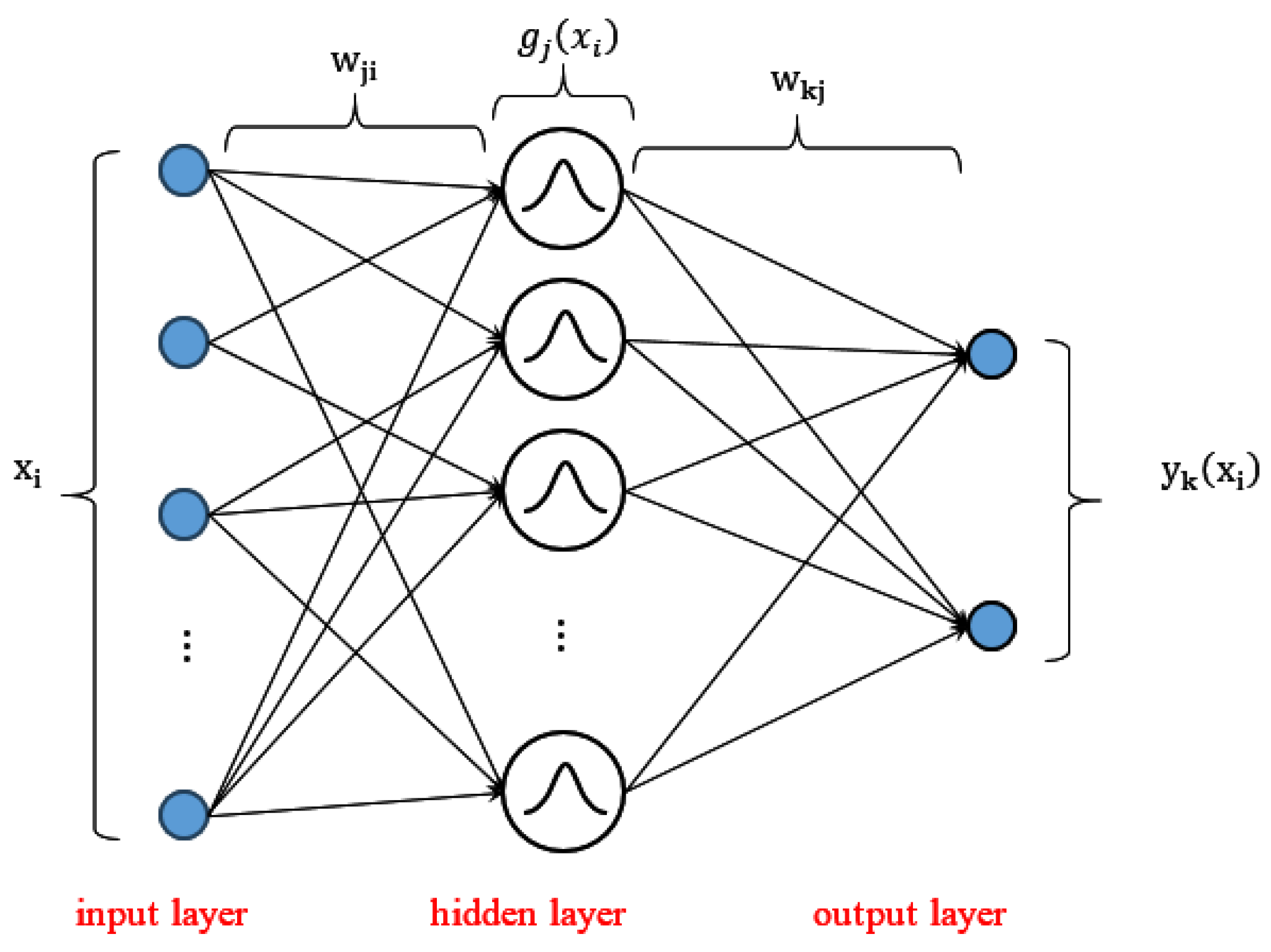
RBF-type neural networks are potent discriminators, meaning they can model complex and non-linear relationships between input and output variables through a radial basis function. An RBF network generally consists of three layers [33]:
-
An input layer that retransmits inputs without distortion and whose neuron number equals the input vector dimension. In this study, we have an input layer with nine neurons receiving the nine gas concentrations.
-
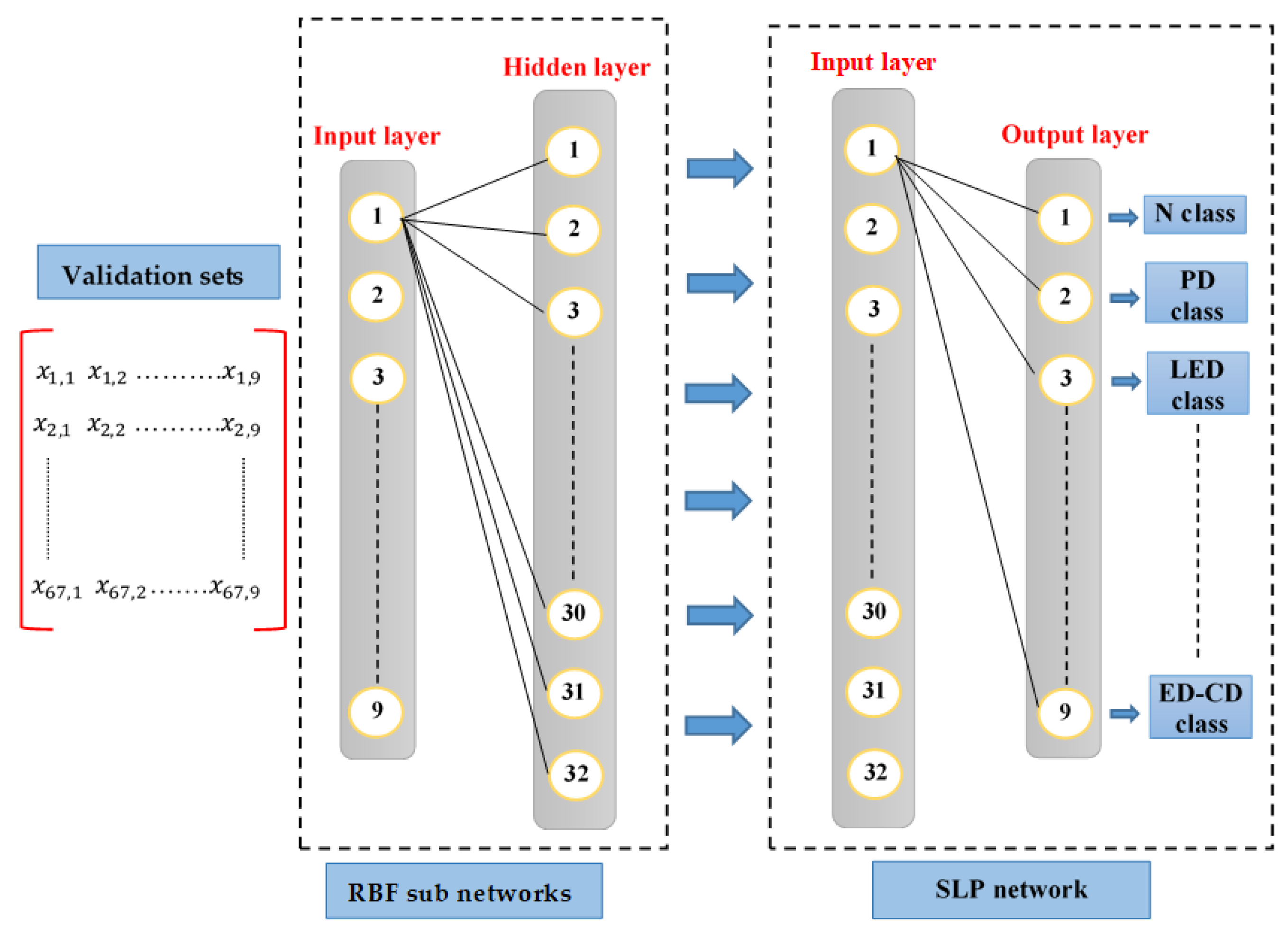
A hidden layer composed of Gaussian-type kernel functions with center C j and a receptive field σ j . Let the example x i ( 1   i   M ) belong to the training set X , the output of the j t h (1 ≤ jM) hidden neuron is given by
      g j ( x i ) = e x p | x i C j 2 2 2 σ j 2 |  
An RBF network’s performance is directly linked to the choice of neuron number in the hidden layer. All the learning examples should be subdivided into subspaces (each containing approximately similar examples), each represented by a center C j . However, when the training examples’ distribution is hard to model, a center C j is assigned to each training example x i , and we therefore find ourselves with centers equal to the learning examples number. That leads to a non-optimal architecture and should be corrected.
-
An output layer with each neuron k representing a fault class or the normal class. The final output of an input vector x i X can be calculated as follows:
  y k ( x i ) = w k 0 + j = 1 M w k j . g j ( x i )    
with w k j as the synaptic weight between a j t h hidden-layer neuron and the output-layer neuron k , and w k 0 as the output error bias. Adjusting the synaptic output weights is another critical element to ensure the good performance of an RBF-type network.
Figure 2 shows a typical RBF network architecture consisting of three layers: an input layer, a hidden layer, and an output layer.
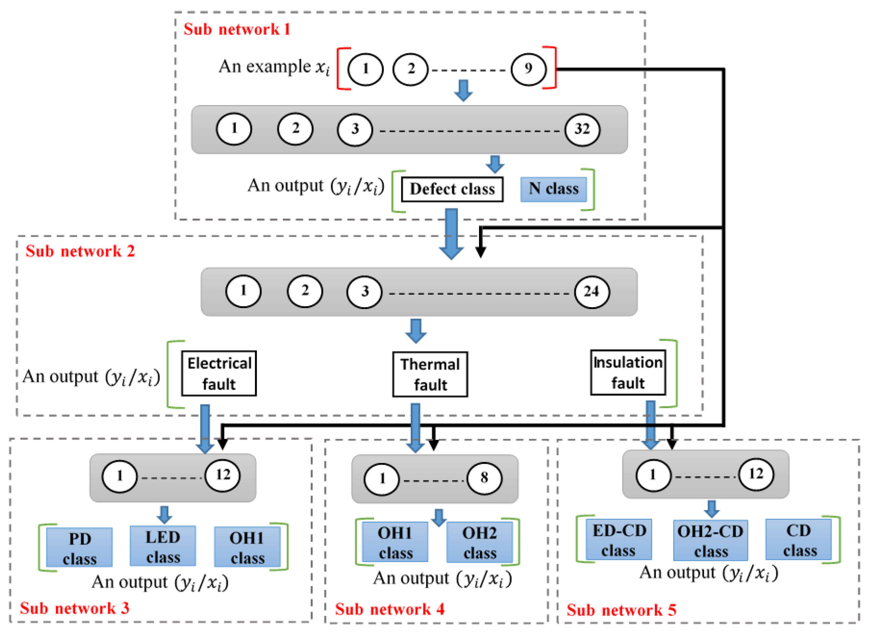
In this study, we considered a hierarchical classifier (Figure 3) the objective being to minimize the global classification task complexity (divide and conquer) and propose a well-established strategy to remedy the imbalanced class problem. The proposed classifier is structured in three stages, each made up of one or more RBF subnetwork(s):
-
Stage 1 consists of a single subnetwork, and it plays the role of a defect detector, effectively separating gas samples with and without defects;
-
Stage 2 also includes a single network, which aims to group the defect samples into three distinct categories: electrical, thermal, and cellulose decomposition;
-
Stage 3 is made up of subnetwork three, responsible for differentiating between electrical faults based on different discharge energy densities; subnetwork 4, able to differentiate between thermal faults according to distinct hot-spot temperatures; and subnetwork 4, which has the role of detecting cellulose decomposition defects with or without the presence of electrical or thermal damage.
To have an optimal overall architecture, the center’s number and the synaptic weights (of the hidden layer) of each subnetwork are optimized. The different steps undertaken are detailed in the two subsections that follow.

3.2. Linde–Buzo–Gray Algorithm

Vector quantization is a well-known technique for data compression. It consists of developing a codebook made up of code vectors, each grouping together highly correlated learning vectors. Indeed, by reducing the redundancy, a new reduced learning set (codebook) is obtained, almost identical in performance (without loss of information) to the original learning set. This sub-section presents the LBG algorithm’s basic foundations [23,24,34].
Let an example x i ( 1   i   N ) belong to a training set X ; let c j ( 1   j   M ) be a vector code belonging to the code book C ; and let ε be a sharing parameter fixed at a minimum value. The LBG algorithm steps can be formulated as follows:
(A)
Initialization
  • Define an initial vector code (initial centroid):
      c 1 = 1 N i = 0 N 1 x i
  • Measure initial distortion:
      d * = 1 N i = 0 N 1 x i c 1 2
(B)
Dividing
  • Double the codebook size by dividing each code vector as follows:
For j = 0 M 1
C j + = c j ( 1 + ε )
C j = c j ( 1 ε )
(C)
Iteration 1
k = 1
  • Determine all the similar amplitude examples with respect to each of the codebook centroids, then form clusters:
      x i X , find Min ( x i c j k 2 ) c j C
Thus, at an iteration k , each example x i is assigned to a centroid C j , and it will be noted that Q ( x i ) = c j ( k ) .
2.
Update the centroids based on the new clusters:
c j ( k + 1 ) = Q ( x i ) = c j ( k ) x i Q ( x i ) = c j ( k ) 1
K + 1 .
3.
Calculate the new distortion:
          d ( k + 1 ) = 1 N i = 0 N 1 x i Q ( x i ) 2
4.
If the threshold ε is lower than d k + 1 d k d k , then go to step (C.1).
5.
Retain the distortion ( d * = d ( k ) ) and centroids (for j = 0 M 1 , c j * = c j ( k ) ) of the current iteration.
(D)
Iteration 2
  • Repeat steps (B) and (C) until the code library size is designed.

3.3. Single-Layer Perceptron [35,36]

The perceptron is a learning model that has proven effective in various classifications and regression problems. It is best known for its simple configuration and speed in reaching the global optimum (rapid convergence). The single-layer perceptron (SLP) constitutes the perceptron’s simplest version; it is made up of
-
An input layer receiving the input vector x i . In this study, the middle layer outputs of a given RBF network constitute the inputs of a given SLP;
-
An output layer comprises threshold functions, each representing a membership category.
The SLP learning algorithm is summarized as follows:
Considering a training set z m = { ( x i , y i ) ,   1 i N } , knowing that y i Y is the desired output of an example x i X .
(A)
Initialization
  • Randomly generate synaptic weights (weight vector) with small values;
  • Set the learning rate value { η } and the desired precision value { ε } ;
  • Calculate the gradient operator on the initial mean squared error (MSE):
      E t ¯ ( w ) = 1 N i = 1 N ( y i ( w T x i + w i 0 ) ) 2    
    where w i 0 is a constant.
(B)
Iterations
  • Update previous error:
      E t 1 ¯ ( w ) = E t ¯ ( w )  
  • For ( x i , y i ) ( X , Y )
    2.1.
    Compute the scalar product between the vector x i and the weight vector w :
    u = w T x i + w i 0
    2.2.
    If y i f ( u ) , update synaptic weights:
    w t = w t 1 + η E ¯ ( w ) w
    where E ¯ ( w ) w = i = 1 N ( y i ( w T x i + w i 0 ) ) ( x i ) and where f is an activation function, whose value is 1 if u > 0 if u > 0 and 0 otherwise.
  • Calculate the new MSE E t ¯ ( w ) by referring to Equation (13).
until ( E t ¯ ( w ) E t 1 ¯ ( w ) < ϵ ) .

3.4. LBG and SLP Algorithms’ Implementation Steps

The steps taken for RBF centers’ quantization with the LBG algorithm, to RBF output-layer connection weights; selection with SLP neural networks and RBF performance test are described below:
-
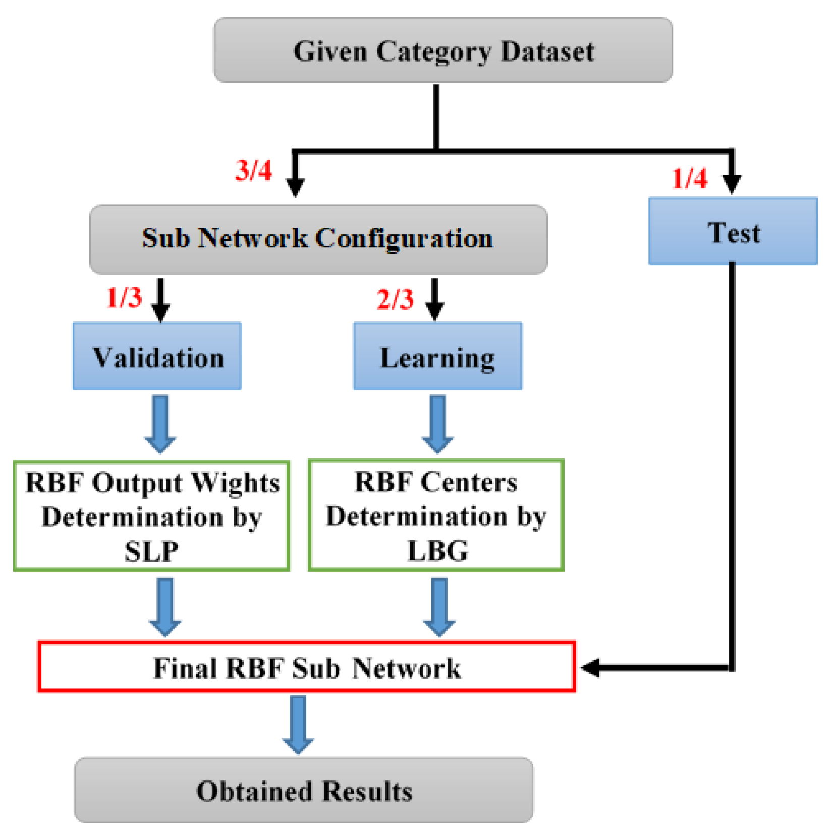
Step 1: The examples distinguished by category (see the global database section II.A) were subdivided randomly and fairly into four parts to implement a process for four cross-validation levels.
At each stage, three sets are retained for the proposed discrimination model configuration: two sets are maintained for the best centroids determination by the LBG algorithm, and one set is for training the SLP neural network (responsible for finding the optimal weights of the output layer). The remaining fourth set is used to test the performance of the obtained hierarchical model (see Figure 4).
-
Step 2: The three sets retained for the configuration (relative to each category) are used to construct five sub-bases, each of which allows the configuration of one of the five subnetworks.
  • Sub-base 1 (for RBF subnetwork 1), includes samples classified as healthy (class 1: 33 examples) and defective (class 2: 168 examples);
  • Sub-base 2 (for RBF subnetwork 2), includes defective samples classified as thermal (class 1: O H 1 + O H 2 = 45 examples), electrical (class 2: P D + L E D + H E D = 66 examples), or cellulose decomposition (class 3: C D + O H 2 C D + E D C D = 57 examples);
  • Sub-base 3 (for RBF subnetwork 3), includes samples with DP defect (class 1: 24 examples), LED defect (class 2: 24 examples), and HED defect (class 3:   18 examples).
  • Sub-base 4 (for RBF subnetwork 4), includes samples with thermal ( t < 700   ° C ) (class 1: 24 examples) and thermal (t > 700 °C) (class 2: 21 examples) defects.
  • Sub-base 5 (for RBF subnetwork 5), includes samples with CD defect (class 1: 24 examples), OH2-CD defect (class 2: 15 examples), and ED-CD defect (class 3: 18 examples).
Once the new bases are defined, the classes of each of them are divided randomly into three: two-thirds (learning set) for the centroids’ definition and one-third (validation set) for the output weights’ determination. This process is repeated for each validation level and each RBF subnetwork (see Table 2).
-
Step 3: The retained centroids are obtained by grouping the most similar input vectors which belong to the same cluster into a single vector using an averaging function (see Equation (11)).
In power transformer diagnostic applications, it does not remain easy to distinguish between samples of different categories due to the high inter-class correlation. It is preferable to apply the LBG algorithm to each class separately (referring, of course, to the reformulated classes in step 2, in accordance with each subnetwork).
On the other hand, to clearly overcome the unbalanced data problem, the same centroid number was retained for each class in the same subnetwork.
Table 3 illustrates the centroid number retained for each subnetwork at a given validation level.
Also, Figure 5 illustrates the centroids distribution based on the training samples.
-
Step 4: An SLP-type network is used to determine the output-layer weights of the retained RBF subnetworks. That makes it possible to overcome the weaknesses of the traditional RBF approach, which is based on a linear combination unable to deal with non-linear cases and which suffers from a fairly long convergence.
  • For each cross-validation step, and each subnetwork, the centroids retained by the LBG algorithm will constitute the hidden-layer neurons of the same subnetwork;
  • Each RBF subnetwork will receive the validation set as input;
  • The centroids (hidden-layer) outputs constitute the SLP inputs;
  • The LSP outputs constitute the membership classes the subnetwork considers;
  • At the end of the learning, the weights obtained by the SLP will constitute the output weights of the final RBF subnetwork.
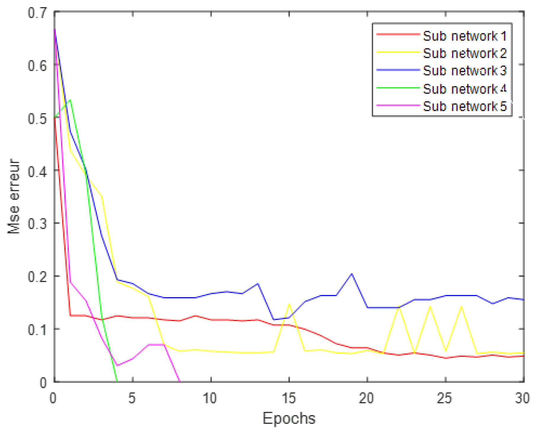
Figure 6 shows the mean square error descent during the SLP network learning phase, and Figure 7 illustrates the process undertaken to determine the synaptic weights (connecting the hidden layer to the output layer) of subnetwork 1.
-
Step 5: Predicting the power transformer health status turns out to be a delicate and complicated task. Indeed, the diagnostic error quantification is generally irregular, complex to evaluate or fix, and varies from one expert to another and from one equipment to another. Therefore, it is preferable and more credible to implement discriminators that return the category’s belonging probabilities rather than the membership class rank (deterministic discrimination). However, RBFs are basically introduced as non-probabilistic classifiers, but it is possible to post-process their outputs in order to obtain posterior probabilities. The following formula needs to be applied to the obtained RBF outputs:
    k     1 , Q ,   y k ˜ = exp ( y k ) exp ( k = 1 Q y k )
with Q as the category number.
-
Step 6: Once all the RBF subnetworks have been formed and optimized, we proceed to the test phase as follows:
  • The samples reserved during testing at each validation level and for each class (see Step 1 and Figure 3) are first merged to form a global test base;
  • The verification of the proposed hierarchical network effectiveness is carried out through each example evaluation at different hierarchy levels;
  • Each RBF subnetwork performance is reported separately in terms of good and bad classification numbers;
  • A test results grouping (by level) is performed at the end so that all examples in the database are tested.

4. Results and Discussion

For an objective performance evaluation of the proposed hierarchical system, a single RBF network was implemented for comparison. The latter is made up of the following:
-
An input layer containing nine neurons, each receiving one dissolved gas;
-
A hidden layer of 72 neurons obtained by applying the LBG algorithm. The retained neuron number is the one which returns the best classification rates (sensitivity); see Table 3;
-
An output layer returning membership probabilities to each of the nine classes considered and whose synaptic neuron weights were optimized by the SLP network.
Table 4 shows that the excellent classification rate is proportional to the kernel function number (sensitivity increased by increasing the center number). For example, by representing each class with a single center, the rates are meager and unacceptable: 65.29%. On the other hand, and to validate the LBG algorithm effectiveness, we assigned a center to each example (for a total of 134 centers per validation level). We see from there that the obtained rates are worse than those obtained with fewer center numbers (72), which can be justified by overtraining.
We also used statistical metrics to validate the proposed approach’s effectiveness with a certain confidence degree, namely
-
Sensitivity: Also called “true positive rate”, the sensitivity quantifies the portion of true positives from the total positive population (taking into consideration even those classified as negative by mistake.
Sensitivity = T P T P + F N  
-
Specificity: Also known as “true negative rate”, it quantifies the true negative portion in relation to the total negative population (even considering samples classified as true by error).
Sensitivity =   T N T N + F P
-
Positive predictive value (PPV): returns the probability that the test is indeed positive if the obtained result is true.
PPV =   T P T P + F P
-
Negative predictive value (NPV): returns the probability that the test is truly negative if the obtained result is negative.
NPV = T N T N + F N  
N.B: The PPV and the NPV can also be deduced from the sensitivity and specificity but in a more complex equation form.
-
Receiver operating characteristic (ROC) curve: allows to draw the torque values’ variation (1-specificity, sensitivity), taking into consideration all the output probabilities generated by the discriminator;
-
Area under the ROC curve (AUROC-95% CI): allows to fully judge the considered discriminator’s performance based on these indicators (in this study case, we refer to posterior probabilities);
-
Student’s test: also called “t-test”, is a parametric tool which can be used to compare the generalization averages of two statistical models, and then it allows to determine whether there exists a significant assessment of one expert over another.
where
TP: samples having the characteristic and whose classification is true;
FN: samples having the characteristic and whose classification is false;
FP: samples not having the characteristic and whose classification is true;
TN: samples not having the characteristic and whose classification is false.
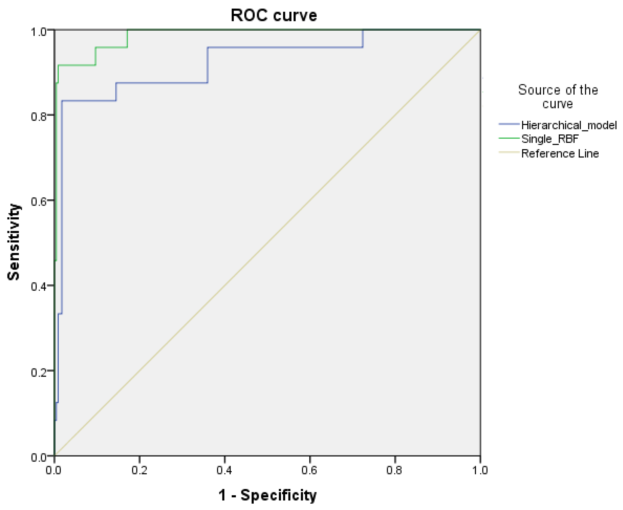
The statistical results reflecting the performance of the proposed hierarchical classifier and that of the single RBF network are exposed in Figure 8 and Figure 9 and in Table 5, Table 6 and Table 7.
Through the two experts’ ROC curves’ evolution shown in Figure 8 and Figure 9, we can clearly see and compare the two models’ performance based on the area under the curve. Indeed, an AUC of 0.5 (50%) means that the classifier is non-informative. An increase in AUC above 0.5 denotes increased generalization capabilities, with a maximum of 1.0 (100%). A decrease in AUC below 0.5 indicates a generalization capabilities’ degradation, with a minimum of 0.0 (0%). Based on the AUROC percentages presented in Table 4, we see that all the hierarchical classifier AUROCs exceed those of the single RBF, with an overall AUROC of 99.16% (p-value < 0.001) (see Table 5) and five cases where the area under the curve is of the order of 100% for the hierarchical model compared to zero cases for the single RBF. Knowing that the ROC curve is a graphical representation of the sensitivity variation to all possible threshold values of the marker considered (in this study, the probabilities are used as a marker), it is easy to deduce that the hierarchical classifier output probabilities (of the winning classes) are higher than those of the single network, which confirms the proposed model robustness. Also, each AUROC was bounded by two values (confidence interval); this will allow us to consider the behavior of a given expert in the face of never-before-seen examples. From this, it can be deduced that the hierarchical model can still efficiently classify new samples with respect to a single RBF and those based on the fact that all AUROC upper bounds of the proposed model can reach 100% for all classes.
The sensitivity is the classification rate per class, and the average of all the sensitivities can be seen as the discrimination model’s overall rate. Theoretically, sensitivity is a crucial parameter for determining the credibility of a classification model. A model with higher sensitivity is more responsive to defects and has a greater capacity to detect the presence of anomalies (the receptive capacity to defect indicators). From Table 5, we notice that the rates by classes of the proposed network unanimously exceed those of the single RBF, and a t-test with p-values < 0.001 validated this difference. As part of this study, the t-test studies the exit probabilities’ average of two given samples and validates from there the difference in the generalization rate, thus proving the output credibility of the proposed hierarchical model. In fact, assigning an example to a category with a high probability is safer than with a low probability.
The FP and FN are critical indicators in diagnostic applications. In fact, it is very dangerous to classify a transformer as healthy when, in reality, it is affected by an anomaly that risks causing irreparable damage. It is, therefore, essential to reduce the FP rate as much as possible; similarly, diagnosing a defective transformer when it is healthy can cost the device downtime when it is not necessary to interrupt its operation, hence the need to minimize as much as possible the FP rate. We note from Table 4 and Table 5 that the FP and FN rates are quite low for the two experts; this can be explained, on the one hand, by the RBF network effectiveness for the power transformer’s diagnosis and, on the other hand, proves the LBG and SLP algorithms’ effectiveness for improving the RBF network’s performance. Nevertheless, the hierarchical model remains more efficient with general FP and FN rates equal to 0.25% and 3.15%, respectively, and with FP and FN rates which are around 0% for the majority of classes. That could be justified because when a hierarchical classification is considered, the generalization task is simplified for the different discriminators by offering them to manage a limited category number (as if we specialize each classifier to accomplish a particular job, a “divide-and-conquer strategy”).
VPP and VPN are important statistical parameters to validate the classifier’s credibility. The PPV returns the rate that samples assigned to a class are actually assigned to that category. If we take, for example, the LED class whose VPP is 96.8%, this implies that among the samples classified, LED 96.8% are actually LED. VPN returns the rate that samples not assigned to a class are actually not assigned to that category. Taking the PD class, the NPV rate is 99.6%; this implies that among the samples classified as non-LED, 99.6% are actually non-LED. By analyzing Table 5, it can be seen that the majority of the hierarchical network VPPs and VPNs are around 100% and are all higher than those of the single network, which therefore validates the obtained results’ credibility.
A temporal study was carried out and reported in the last line of Table 6 to study the feasibility of embedding the implemented model in real applications. The hierarchical network learning time is significantly smaller than that of the single RBF network, which is due to the subnetwork structure’s simplicity. The big surprise is that the generalization rates are practically identical despite the sample’s passage by level, indicating the proposed system’s flexibility.
Also, to properly evaluate the proposed hierarchical model, each subnetwork’s performances are reported in Table 7. Ideal performances can be observed for two subnetworks, 1 and 5, and delightful performances for the three remaining subnetworks, which once again proves the effectiveness of hierarchical implementation to ensure the efficient diagnosis of power transformers.
Finally, it is essential to position the proposed work in relation to previous research, which is quite similar to this study. Thus, to simplify the comparison, we present in Table 8 a summary of selected methods. Also, with the aim of an adequate comparison, we summarize our method’s key points in the last lines of Table 7. From these results, we see that the obtained generalization rate, the classes, and the number of test example considered are higher than all the methods except studies [27,31,32].
-
Study [27] considers more examples; simultaneously, the authors obtained generalization rates higher than ours. However, the authors use a lower-class number than ours, which could facilitate the classification task and justify the high rates. Also, the present study considers statistical parameters and confidence intervals, which promise similar or even better results for a more extensive data set;
-
Study [31] considered more test examples but fewer categories than the present study, and it proposed a low test rate compared to ours, whereas study [32] treats the same class number as this study with more test examples and presents poorer generalization results. But once again, we recall that according to the statistical tests carried out, the results we obtained could be found with more test examples.

5. Conclusions

Power transformers are considered the most important elements in an energy infrastructure. Their proper functioning ensures a reliable, safe, and high-quality supply of electrical energy to users. The dissolved gas analysis (DGA) approach is widely recognized as one of the most effective methods for anticipating faults in power transformers. It analyzes dissolved gases in the insulating oil at a low cost. The present study establishes a hierarchical classification model consisting of five RBF-type subnetworks, each responsible for a specific classification task. Each subnetwork was configured to provide the best performance. The LBG algorithm application determined the kernel functions, and the SLP network decided the hidden layer synaptic weights. The proposed model performance was compared to that of a single RBF network whose architecture was also optimized.
Unlike the single network, the proposed hierarchical fault diagnosis model helped improve the performance significantly, particularly the overall generalization rate, which increased by more than 5% (statistical tests validated this observation) and achieved more balanced fault-finding results on unbalanced data sets. Furthermore, the performance superiority of the proposed fault-detection model indicates superiority over the research reported in the literature. The risk of mistaken diagnostics can therefore be reduced, while the likelihood of identifying incipient failures before they lead to transformer failures is maximized.
Nevertheless, this study opens the door to several future perspectives and could be reinforced by further work, such as the following: implementing other approaches to optimize the RBF hyperparameters for comparison; conducting a comparative study between various kernel machines, such as SVM, which are considered highly suitable for diagnosing transformer issues from DGA; incorporating anthologies (antecedents dictionary) for regular transformer monitoring; and introducing Internet of Things (IoT) services to enable real-time implementation and monitoring.

Author Contributions

Conceptualization, M.H.; methodology, M.H.; software, M.H.; validation, M.H. and I.S.B.; formal analysis, M.H., I.S.B., F.M., M.B. and I.F.; investigation, M.H.; resources, M.H.; data curation, M.H.; writing—original draft preparation, M.H.; writing—review and editing, M.H., I.F., F.M., M.B. and I.S.B.; supervision, M.B., I.F. and F.M.; project administration, M.B.; funding acquisition, M.H. and M.B. All authors have read and agreed to the published version of the manuscript.

Funding

This work was supported by the PRFU-C00L07EP31022010001 project and the General Directorate for Scientific Research and Technological Development (DGRSDT).

Data Availability Statement

The data used in this research are real samples of oil extracted from power transformers belonging to the electricity and gas company Sonelgaz Transport Electricity (STE) in western Algeria.

Conflicts of Interest

The authors declare no conflicts of interest.

References

  1. Wang, G.; Liu, Y.; Chen, X.; Yan, Q.; Sui, H.; Ma, C.; Zhang, J. Power transformer fault diagnosis system based on Internet of Things. J. Wirel. Commun. Netw. 2021, 2021, 21. [Google Scholar] [CrossRef]
  2. Wani, S.A.; Rana, A.S.; Sohail, S.; Rahman, O.; Parveen, S.; Khan, S.A. Advances in DGA based condition monitoring of transformers: A review. Renew. Sustain. Energy Rev. 2021, 149, 111347. [Google Scholar] [CrossRef]
  3. Abbasi, A.R. Fault detection and diagnosis in power transformers: A comprehensive review and classification of publications and methods. Electr. Power Syst. Res. 2022, 209, 107990. [Google Scholar] [CrossRef]
  4. Sun, H.C.; Huang, Y.C.; Huang, C.M. Fault Diagnosis of Power Transformers Using Computational Intelligence: A Review. Energy Procedia 2012, 14, 1226–1231. [Google Scholar] [CrossRef]
  5. Muniz, R.N.; Costa Júnior, C.T.; Buratto, W.G.; Nied, A.; González, G.V. The Sustainability Concept: A Review Fo-cusing on Energy. Sustainability 2023, 15, 14049. [Google Scholar] [CrossRef]
  6. Islam, M.; Lee, G.; Hettiwatte, S.N. A nearest neighbour clustering approach for incipient fault diagnosis of power transformers. Electr. Eng. 2017, 99, 1109–1119. [Google Scholar] [CrossRef]
  7. Rogers, R.R. IEEE and IEC codes to interpret incipient faults in transformers, using gas in oil analysis. IEEE Trans. Electr. Insul. 1978, EL-13, 349–354. [Google Scholar] [CrossRef]
  8. Irungu, G.K.; Akumu, A.O.; Munda, J.L. A new fault diagnostic technique in oil-filled electrical equipment; the dual of Duval triangle. IEEE Trans. Dielectr. Electr. Insul. 2016, 23, 3405–3410. [Google Scholar] [CrossRef]
  9. Khan, S.A.; Equbal, M.D.; Islam, T.A. Comprehensive comparative study of DGA based ANFIS models. IEEE Trans. Dielectr. Electr. Insul. 2015, 22, 590–596. [Google Scholar] [CrossRef]
  10. Peimankar, A.; Weddell, S.J.; Thahirah, J.; Lapthorn, A.C. Evolutionary Multi-Objective Fault Diagnosis of Power Transformers. Swarm Evol. Comput. 2017, 36, 62–75. [Google Scholar] [CrossRef]
  11. Abdo, A.; Liu, H.; Zhang, H.; Guo, J.; Li, Q. A new model of faults classification in power transformers based on data optimization method. Electr. Power Syst. Res. 2021, 200, 107446. [Google Scholar] [CrossRef]
  12. Hua, Y.; Sun, Y.; Xu, G.; Sun, S.; Wang, E.; Pang, Y. A fault diagnostic method for oil-immersed transformer based on multiple probabilistic output algorithms and improved DS evidence theory. Int. J. Electr. Power Energy Syst. 2022, 137, 107828. [Google Scholar] [CrossRef]
  13. Guardado, J.L.; Naredo, J.L.; Moreno, P.; Fuerte, C.R. A Comparative Study of Neural Network Efficiency in Power Transformers Diagnosis Using Dissolved Gas Analysis. IEEE Trans. Power Deliv. 2001, 16, 643–647. [Google Scholar] [CrossRef]
  14. Han, X.; Ma, S.; Shi, Z.; An, G.; Du, Z.; Zhao, C. A Novel Power Transformer Fault Diagnosis Model Based on Harris-Hawks-Optimization Algorithm Optimized Kernel Extreme Learning Machine. J. Electr. Eng. Technol. 2022, 17, 1993–2001. [Google Scholar] [CrossRef]
  15. Li, S.; Wu, G.; Gao, B.; Hao, C.; Xin, D.; Yin, X. Interpretation of DGA for Transformer Fault Diagnosis with Complementary SaE-ELM and Arctangent Transform. IEEE Trans. Dielectr. Electr. Insulation. 2016, 23, 586–595. [Google Scholar] [CrossRef]
  16. Le, X.; Yijun, Z.; Keyu, Y.; Mingzhen, S.; Wenbo, L.; Dong, L. Interpretation of DGA for Transformer Fault Diagnosis with Step-by-step feature selection and SCA-RVM. In Proceedings of the IEEE 16th Conference on Industrial Electronics and Applications, Chengdu, China, 1–4 August 2021. [Google Scholar] [CrossRef]
  17. Zhang, Y.; Li, X.; Zheng, H.; Yao, H.; Liu, J.; Zhang, C.; Peng, H.; Jiao, J. A Fault Diagnosis Model of Power Transformers Based on Dissolved Gas Analysis Features Selection and Improved Krill Herd Algorithm Optimized Support Vector Machine. IEEE Access 2019, 7, 102803–102811. [Google Scholar] [CrossRef]
  18. Kari, T.; Gao, W.; Zhao, D.; Abiderexiti, K.; Mo, W.; Wang, Y.; Luan, L. Hybrid feature selection approach for power transformer fault diagnosis based on support vector machine and genetic algorithm. Inst. Eng. Technol. 2018, 12, 5672–5680. [Google Scholar] [CrossRef]
  19. Hendel, M.; Meghnefi, F.; Senoussaoui, M.A.; Fofana, I.; Brahami, M. Using Generic Direct M-SVM Model Improved by Kohonen Map and Dempster–Shafer Theory to Enhance Power Transformers Diagnostic. Sustainability 2023, 15, 15453. [Google Scholar] [CrossRef]
  20. Nanfak, A.; Samuel, E.; Fofana, I.; Meghnefi, F.; Ngaleu, M.G.; Hubert Kom, C. Traditional fault diagnosis methods for mineral oil-immersed power transformer based on dissolved gas analysis: Past, present and future. IET Nanodielectrics 2024, 1–34. [Google Scholar] [CrossRef]
  21. Meng, K.; Dong, Z.Y.; Wang, D.H.; Wong, K.P. A Self-Adaptive RBF Neural Network Classifier for Transformer Fault Analysis. IEEE Trans. Power Syst. 2010, 25, 1350–1360. [Google Scholar] [CrossRef]
  22. Zhang, J.; Pan, H.; Huang, H.; Liu, S. Electric Power Transformer Fault Diagnosis using OLS based Radial Basis Function Neural Network. In Proceedings of the IEEE International Conference on Industrial Technology, Chengdu, China, 21–24 April 2008. [Google Scholar] [CrossRef]
  23. Guo, Y.J.; Sun, L.H.; Liang, Y.C.; Ran, H.C.; Sun, H.Q. The fault diagnosis of power transformer based on improved RBF neural network. In Proceedings of the IEEE Sixth International Conference on Machine Learning and Cybernetics, Hong Kong, China, 19–22 August 2007. [Google Scholar] [CrossRef]
  24. Linde, Y.; Buzo, A.; Gray, R.M. An Algorithm for Vector Quantizer Design. IEEE Trans. Commun. 1980, 28, 84–95. [Google Scholar] [CrossRef]
  25. Jack, R.; Knutson, Y.; Choo, C.Y. Feature based compression of vector quantized codebooks and data for optimal image compression. In Proceedings of the IEEE International Symposium on Circuits and Systems, Chicago, IL, USA, 3–6 May 1993. [Google Scholar] [CrossRef]
  26. Staiano, A.; Tagliaferri, R.; Pedrycz, W. Improving RBF networks performance in regression tasks by means of a supervised fuzzy clustering. Neurocomputing 2006, 69, 1570–1581. [Google Scholar] [CrossRef]
  27. Obulareddy, S.; Munagala, S.K. Improved Radial Basis Function (RBF) Classifier for Power Transformer Winding Fault Classification. Innov. Electr. Electron. Eng. 2022, 894, 587–601. [Google Scholar] [CrossRef]
  28. Chen, S.; Wu, Y.; Luk, B.L. Combined genetic algorithm optimization and regularized orthogonal least squares learning for radial basis function net works. IEEE Trans. Neural Netw. 1999, 10, 1239–1243. [Google Scholar] [CrossRef]
  29. Chng, E.S.; Chen, S.; Mulgrew, B. Gradient radial basis function networks for non linear and non stationary time series prediction. IEEE Trans. Neural Netw. 1996, 7, 190–194. [Google Scholar] [CrossRef]
  30. Cui, Y.; Ma, H.; Saha, T. Improvement of Power Transformer Insulation Diagnosis Using Oil Characteristics Data Preprocessed by SMOTEBoost Technique. IEEE Trans. Dielectr. Electr. Insul. 2014, 21, 2363–2373. [Google Scholar] [CrossRef]
  31. Kherif, O.; Benmahamed, Y.; Teguar, M.; Boubakeur, A.; Ghoneim, S.M. Accuracy Improvement of Power Transformer Faults Diagnostic Using KNN Classifier With Decision Tree Principle. IEEE Access 2021, 9, 81693–81701. [Google Scholar] [CrossRef]
  32. Su, L.; Cui, Y.; Yu1, Z.; Chen, L.; Xu, P.; Hou, H.; Sheng, G. A Power Transformer Fault Diagnosis Method Based on Hierarchical Classification and Ensemble Learning. J. Phys. Conf. Ser. 2019, 1346, 012045. [Google Scholar] [CrossRef]
  33. Wurzberger, F.; Schwenker, F. Learning in Deep Radial Basis Function Networks. Entropy 2024, 26, 368. [Google Scholar] [CrossRef]
  34. Bilal, M.; Ullah, Z.; Mujahid, O.; Fouzder, T. Fast Linde–Buzo–Gray (FLBG) Algorithm for Image Compression through Rescaling Using Bilinear Interpolation. J. Imaging 2024, 10, 124. [Google Scholar] [CrossRef]
  35. Yousaf, M.Z.; Khalid, S.; Tahir, M.F.; Tzes, A.; Raza, A. A novel dc fault protection scheme based on intelligent network for meshed dc grids, International. J. Electr. Power Energy Syst. 2023, 154, 109423. [Google Scholar] [CrossRef]
  36. Yousaf, M.Z.; Tahir, M.F.; Raza, A.; Khan, M.A.; Badshah, F. Intelligent Sensors for dc Fault Location Scheme Based on Optimized Intelligent Architecture for HVdc Systems. Sensors 2022, 22, 9936. [Google Scholar] [CrossRef]
Figure 1. Z-score normalization result.
Energies 17 03171 g001
Figure 2. An RBF network architecture.
Energies 17 03171 g002
Figure 3. The proposed hierarchical model organization (The grey area represents each subnetwork’s hidden layer).
Energies 17 03171 g003
Figure 4. Given category dataset distribution (for one cross-validation stage).
Energies 17 03171 g004
Figure 5. The centroids distribution for subnetwork 1.
Energies 17 03171 g005
Figure 6. Subnetworks’ MSE descent.
Energies 17 03171 g006
Figure 7. The process of determining the subnetwork 1 synaptic weights.
Energies 17 03171 g007
Figure 8. HED class ROC curve.
Energies 17 03171 g008
Figure 9. Normal class ROC curve.
Energies 17 03171 g009
Table 1. Used database distribution.
DefectAbbreviationInterpretationSample
NormalNHealthy samples category44
ElectricalPDPartial Discharge32
LEDLow-energy discharge32
HEDHigh-energy discharge24
ThermalOH1 Thermal   fault   ( t < 700   ° C ) 32
OH2 Thermal   fault   ( t > 700   ° C ) 28
Cellulose decompositionCDCellulose degradation32
OH2-CDThermal (t > 700 °C) and cellulose degradation20
ED-CDEnergy discharge and cellulose degradation24
Table 2. Sub-bases, learning sets, and validation sets.
DefectRetained CategorySub-BasesLearning SetsValidation Sets
Subnetwork 1Healthy samples 332211
Defect samples 16811256
Subnetwork 2Electric 664422
Thermal 453015
Cellulose degradation 573819
Subnetwork 3PD 24168
LED 24168
HED 18126
Subnetwork 4OH1 24168
OH2 21147
Subnetwork 5CD 24168
OH2-CD 15105
ED-CD 18126
Table 3. The centroids distribution.
DefectRetained CategoryInitial ExampleRetained Centers
Subnetwork 1Healthy samples 2216
Defect samples 11216
Subnetwork 2Electric 448
Thermal 308
Cellulose degradation 388
Subnetwork 3PD 164
LED 164
HED 124
Subnetwork 4OH1 164
OH2 144
Subnetwork 5CD 164
OH2-CD 104
ED-CD 124
Table 4. Average sensitivity of the single RBF model according to the center number.
Kernel Functions NumberSensitivity (%)
965.29
1877.23
3681.71
7291.79
13483.95
Table 5. Single RBF and proposed hierarchical model performances (all AUROC p-value < 0.001).
ClassStatistical ParametersHierarchical ModelSingle RBF
NAUROC100 [100–100]96.4 [92.3–100]
Sensitivity10095.5
Specificity10099.1
False positive00.9
False negative04.5
VPP10095.5
VPN10099.1
PDAUROC99.7 [99.1–100]96.5 [92.6–100]
Sensitivity96.993.8
Specificity99.699.2
False positive0.40.8
False negative3.16.3
VPP96.993.8
VPN99.699.2
LEDAUROC99.3 [98.3–100]95 [90.4–99.6]
Sensitivity93.890.6
Specificity99.698.7
False positive0.41.3
False negative6.39.4
VPP96.890.6
VPN99.298.7
HEDAUROC98.7 [97–100]92.3 [85.5–99.1]
Sensitivity91.783.3
Specificity99.298.4
False positive0.81.6
False negative8.316.7
VPP91.783.3
VPN99.298.4
OH1AUROC100 [100–100]98.4 [95.7–100]
Sensitivity10096.9
Specificity10099.2
False positive00.8
False negative03.1
VPP10093.9
VPN10099.6
OH2AUROC94.8 [88–100]92.5 [85.7–99.4]
Sensitivity89.385.7
Specificity10098.8
False positive01.3
False negative10.714.3
VPP10088.9
VPN98.898.3
CDAUROC100 [100–100]99.4 [98.5–100]
Sensitivity10096.9
Specificity10099.2
False positive00.8
False negative03.1
VPP10093.9
VPN10099.6
OH2-CDAUROC100 [100–100]96.3 [91.5–100]
Sensitivity10090
Specificity10098.8
False positive01.2
False negative010
VPP10085.7
VPN10099.2
ED-CDAUROC100 [100–100]96.5 [92.5–100]
Sensitivity10087.5
Specificity99.299.2
False positive0.80.8
False negative012.5
VPP92.391.3
VPN10098.8
Table 6. Average performances of single RBF and the proposed hierarchical model.
Hierarchical ModelSingle RBF
AUROC99.16 [98.04–100]95.92 [91.63–99.78]
Sensitivity96.8591.13
Specificity99.7398.95
False positive0.271.05
False negative3.158.87
VPP97.5290.77
VPN99.6498.99
Learning time (s)105
± 0.015
398
± 0.043
Execution time (s)0.013
± 0.002
0.022
± 0.006
Table 7. Average performances of RBF subnetworks.
Subnetwork 1Subnetwork 2Subnetwork 3Subnetwork 4Subnetwork 5
AUROC (95% CI)
(p-value < 0.001)
100 [100–100]99.33 [98.57–100]99.13 [97.83–100]99.45 [98.55–100]100 [100–100]
Sensitivity10097.7797.9398.1100
Specificity10098.998.8398.1100
False positive00.51.171.90
False negative02.232.071.90
VPP02.232.071.90
VPN10098.8798.898.5100
Table 8. A comparative study.
MethodClasses
Number
Examples
Number
Generalization Rate (%)
RBF + OLS [22]621491
RBF + k-AC method [23]52290.90
KNN classifier with decision tree principle [31]650192.5
Hierarchical classification + ensemble learning [32]9457Back propagation NN: 98.59
SVM: 79.65
Random forest: 76.81
Proposed method: 90.37
RBF + FCM + QPSO [21]45082.64
{SVM, C45, RBF, KNN} + SMOTE [30]4181C45: 98
KNN: 84
RBF: 84
SVM: 98
RBF + {PSO, Gradient, FFA, IFFA} [27]5580GD: 78.73
PSO: 90.22
FFA: 92.52
IFFA: 98.27
RBF + LBG + SLP9256Single RBF: 91.13
Hierarchical model: 96.85
Disclaimer/Publisher’s Note: The statements, opinions and data contained in all publications are solely those of the individual author(s) and contributor(s) and not of MDPI and/or the editor(s). MDPI and/or the editor(s) disclaim responsibility for any injury to people or property resulting from any ideas, methods, instructions or products referred to in the content.