Research on the Throttling Performance and Anti-Erosion Structure of Trapezoidal Throttle Orifices

Abstract

The throttling performance of conventional throttle orifice structures of fluid control valves is very low. Therefore, this paper proposes a novel trapezoidal throttle orifice with excellent throttling performance. The effect of the taper of the throttle orifice on the erosion was researched. Firstly, two schemes of trapezoidal throttle orifice were proposed according to the fluid control valve. Secondly, the excellent throttling performance of the trapezoidal throttle orifice was compared and optimized. Finally, a numerical simulation method of the erosion-resistant ability of the trapezoidal throttle orifice was established. It was found that for the same throttling area, the differential pressure of the trapezoidal orifice was higher than that of the conventional rectangular orifice by about 18.6%. The taper had little effect on the gas production, which increased by only 3.3% during the 10° to 30° change. The maximum erosion was firstly reduced and then increased with increases in the angle from 0 to 25°of the taper. Moreover, the minimum was achieved at about a 20° taper angle. The above research methods provide a theoretical basis for optimizing the size and structure of orifices and the sealing reliability of fluid control valves.

1. Introduction

With the expansion of oil and gas development, horizontal well technology has become the mainstream oil and gas extraction technique [1,2]. Compared with straight wells, horizontal wells have a larger contact area with the oil and gas segment. Thus, the oil unloading area is more prominent, and the oil and gas production of horizontal wells is about three times greater than that of straight wells [3]. However, with the increasing length of horizontal wells, there is a severe imbalance of oil and gas exploration in each production segment of long horizontal wells. Against this background, engineers have proposed an intelligent completion technology capable of the real-time monitoring of downhole information, controlling the flow of production fluids downhole, and eliminating the need for manually interfering operations such as workovers. Intelligent completion technology enables production managers to manage oil, gas, and water formations in an orderly manner. Intelligent completion technology also facilitates the control of fluid flow from the bottom layer to the reservoir according to the manager’s intention. Engineers can use this technology for both fractional and combined recovery. Moreover, it can also realize segmented sealing, selective fracturing and acidizing, and repetitive fracturing and acidizing [4,5,6,7,8].

As the core tool of intelligent completion technology, fluid control valves can mainly be categorized into active (fluid control valves) and passive (flow control devices) according to the throttle method [9,10,11]. Engineers primarily use passive fluid control devices to solve water breakthrough problems in horizontal wells. It is mainly those associated with horizontal wells and multi-branch wells. The principle of operation is to increase the resistance to fluid flow in the high-permeability zone of horizontal wells through the differential pressure generated by multiple flow paths, therefore reducing the volume of fluid flowing into the wellbore. However, this device operates primarily by passive fluid regulation relying on fluid pressure differentials. The active fluid control valve adjusts the differential pressure of each production segment of horizontal wells by actively changing the throttle orifice’s opening to achieve balanced exploitation. Figure 1 is a three-dimensional structure schematic of the active fluid control valve.

Engineers open or close the valve primarily by moving the sliding sleeve inside the fluid control valve. In Figure 1, the electric control section is primarily used to install the control board, power supply, and other components. The optical fiber measurement section is mainly used to measure the fluid parameters of the formation. The oil tank is primarily used to store hydraulic oil. The hydraulic power source is mainly used to provide the power to move the sliding sleeve. The hydraulic power source injects hydraulic oil into the hydraulic chambers at the left and right sides of the sliding sleeve by drawing hydraulic oil from the tank. The hydraulic oil then pushes the sliding sleeve to move between the outer and inner cylinders in the annular region. At the same time, the sliding sleeve is provided with some throttle orifices and some fracture orifices. The movement of the sliding sleeve leads the throttle orifices or fracture orifices to align with the overflow orifices on the outer cylinder and the inner cylinder. Finally, this causes the valve to switch on and off or to change working conditions.

Throttle orifices are mainly used in oil and gas extraction, and fracture orifices are primarily utilized in fracturing. When the fluid in the formation enters the throttle orifice, the flow velocity will increase rapidly due to the sudden space reduction. Then, the fluid with enormous flow velocity will carry solid particles to hit the wall of throttle orifices. The particles hit the wall and cut a small portion of the material, eventually leaving pits in the throttle orifice’s wall, where erosion occurs. Erosion is prevalent in almost all types of orifices because the dramatic increase in fluid flow velocity at the orifice is a significant cause. Currently, the three main industry throttle orifice shapes are rectangular, elliptic, and circular.

Excellent throttling performance is the basis for fluid control valves to regulate the production segments of horizontal wells efficiently. Most existing studies on improving throttling performance focus on optimizing the design of the valve body structure of fluid control valves [12,13,14]. In addition, Chuan Li et al. [15] established a flow model of a fluid control valve to optimize the throttling performance. Jinhui Zhou et al. [16] investigated the effect of different parameters on the throttle efficiency. None of the above studies could optimize the structure and parameters of throttle orifices. Dong Guo [12] analyzed the internal flow field of a single fluid control valve and the throttle area of longitudinal throttle orifices through his study. However, the throttling differential pressure of the orifices was relatively low. Therefore, there is still a lack of reports on the research of the structural design and erosion resistance of throttle orifices. Conducting design research on throttle orifices to improve throttling performance is significant.

This paper proposes a novel trapezoidal throttle orifice with excellent throttling performance. Furthermore, because the erosion of throttle orifices is the leading cause of the seal failure of fluid control valves, it is of great significance to research the erosion resistance of trapezoidal throttle orifices. Based on this, two trapezoidal orifice schemes were proposed according to the structure and working principle of the fluid control valve. The throttling differential pressures of trapezoidal and conventional orifices were compared to evaluate the excellent throttling performance of trapezoidal orifices. At the same time, the best trapezoidal throttle orifice scheme was selected. Finally, the numerical simulation method was used to research the effect of different tapers on the erosion resistant capability of the orifice. The above research methods and results can provide a theoretical basis for optimizing the size and structure of throttle orifices and the seal reliability design of fluid control valves.

2. Mathematical Model

2.1. Continuity and Momentum Equations

This research set natural gas as the fluid medium used for this numerical simulation. The density of the natural gas downhole was 0.67 kg/m³ and the viscosity was 0.03 mPa·s [17]. The fluid flow had to satisfy the continuity, momentum, and energy equations [18]. The energy equation was not used in the numerical simulation because this research did not consider the temperature change.

The natural gas flow in the fluid control valve was regarded as an incompressible fluid, and the continuity equation can be obtained as:

$$\frac{\partial \rho }{\partial t}+\frac{\partial (\rho u)}{\partial x}+\frac{\partial (\rho v)}{\partial y}+\frac{\partial (\rho w)}{\partial z}=0$$

(1)

In the above equation, ρ is the fluid density, kg/m³; t is the time interval, s; x, y, and z are the three directions of the coordinate axes respectively; and u, v, and w are the velocity components of the fluid microparticles in the x, y, and z directions, m/s.

The fluid in the fluid control valve was incompressible and the density was constant. Therefore, the derivative of the fluid density concerning time in Equation (1) is 0.

The momentum equation is as follows:

$$\left\{\begin{array}{l}\frac{\partial (\rho u)}{\partial t}+\frac{\partial (\rho uu)}{\partial x}+\frac{\partial (\rho uv)}{\partial y}+\frac{\partial (\rho uw)}{\partial z}=-\frac{\partial p}{\partial x}+\frac{\partial {\tau }_{xx}}{\partial x}+\frac{\partial {\tau }_{yx}}{\partial y}+\frac{\partial {\tau }_{zx}}{\partial z}+\rho f_x\\ \frac{\partial (\rho v)}{\partial t}+\frac{\partial (\rho vu)}{\partial x}+\frac{\partial (\rho vv)}{\partial y}+\frac{\partial (\rho vw)}{\partial z}=-\frac{\partial p}{\partial y}+\frac{\partial {\tau }_{xy}}{\partial x}+\frac{\partial {\tau }_{yy}}{\partial y}+\frac{\partial {\tau }_{zy}}{\partial z}+\rho f_y\\ \frac{\partial (\rho w)}{\partial t}+\frac{\partial (\rho wu)}{\partial x}+\frac{\partial (\rho wv)}{\partial y}+\frac{\partial (\rho ww)}{\partial z}=-\frac{\partial p}{\partial z}+\frac{\partial {\tau }_{xz}}{\partial x}+\frac{\partial {\tau }_{yz}}{\partial y}+\frac{\partial {\tau }_{zz}}{\partial z}+\rho f_z\end{array}\right.$$

(2)

In the above equation, f_x, f_y, and f_z are the components of the volume force in the x, y, and z directions respectively, N; p is the pressure, Pa; and τ_xx, τ_xy, and τ_xz are the components of the stress in the x, y, and z direction on the face perpendicular to the x-axis, respectively. For example, the first subscript x of τ_xx represents the surface where the stress is perpendicular to the x-axis. The second subscript x indicates the direction of the component force. The principle is the same for the rest of the similar parameters. Figure 2 illustrates the direction of the parameters in Equation (2).

2.2. Turbulence Model

To perform a numerical simulation, it is necessary to first determine the state of motion of the fluid within the fluid control valve. The formula for the Reynolds number is shown below:

$$\mathrm{Re}=\frac{\rho uL}{v}$$

(3)

In the above equation, L is the characteristic length, m, and Re is the Reynolds number. The fluid medium was natural gas with a density of 0.67 kg/m³ and a kinematic viscosity of 0.03 mPa·s. Natural gas generally flowed at a high speed in the valve; thus, the fluid flow speed was set to 18 m/s. The characteristic length took the value of 0.108 m. Substituting the relevant parameters gave a Reynolds number of 43,416. The Reynolds number was higher than 2300; therefore, the flow of natural gas in the fluid control valves was turbulent.

The flow of natural gas in fluid control valves during natural gas extraction is characterized by significant turbulence [19,20]. Therefore, the Realizable k–ε model, the most widely used in engineering applications, was chosen for numerical simulations [21,22]. The Realizable k–ε model suits turbulent flow with high Reynolds number in fluid control valves [23,24]. The equations of turbulence kinetic energy, k, and dissipation rate, ε, are shown in Equations (4) and (5):

$$\frac{\partial \left(\rho k\right)}{\partial t}+\frac{\partial \left(\rho k{u}_i\right)}{\partial x_i}=\frac{\partial }{\partial x_j}\left[{\sigma }_k{\mu }_t\frac{\partial }{\partial x_j}\right]+G_k+G_b-\rho \epsilon -Y_M+S_k$$

(4)

$$\frac{\partial \left(\rho \epsilon \right)}{\partial t}+\frac{\partial \left(\rho \epsilon u_i\right)}{\partial x_i}=\frac{\partial }{\partial x_j}\left[{\sigma }_{\epsilon }{\mu }_t\frac{\partial \epsilon }{\partial x_j}\right]+C_{1\epsilon }\frac{\epsilon }{k}\left(G_k+C_{3\epsilon }{G}_b\right)-C_{2\epsilon }\rho \frac{{\epsilon }^2}{k}-R_{\epsilon }+S_{\epsilon }$$

(5)

where k is the turbulent kinetic energy, J; G_k is the turbulent kinetic energy generated by laminar velocity gradient, J; G_b is the turbulent kinetic energy generated by buoyancy, J; x_i and x_j are the displacement of the fluid in the directions of i and j, respectively, m; u_i is the flow velocity, m/s; Y_M is the effect of pulsating expansion of compressible turbulence on the total dissipation rate, J, with incompressible fluid taking the value of 0; μ_t is the effective viscosity, kg/(m-s); ε is the turbulent dissipation rate, J/s; σ_k and σ_ε are the k equation and ε equation turbulent Prandtl number, J; C_1ε, C_2ε, and C_3ε are the empirical constants; S_k and S_ε are the user-defined original terms; and R_ε is the ε function.

2.3. Erosion Model

The calculation methods of the erosion can mainly be categorized in computational fluid dynamics [25]: the Euler–Lagrange method and the Euler–Euler method. The Euler–Lagrange method defines fluid and particles as continuous and discrete phases; it applies to the case where the volume fraction of particles is less than 10% to 12%. The Eulerian-Eulerian method considers particle–particle interactions and treats particles as a continuous phase. There is no restriction on the particle volume fraction requirement, but the Euler–Euler method is generally used when the particles are denser. The sand content in natural gas is usually small; thus, this study used the Euler–Lagrange method for the numerical simulation.

Finnie proposed the theory of the micro-cutting erosion model [26]; the erosion rate of solid particles impacting a pipe wall can be calculated by Equation (6).

$$E_R=1.559e^{-6}{B}^{-0.59}{F}_s{v}^{1.73}f(\alpha )$$

(6)

In the above formula: E_R is the erosion rate, kg/(m²·s); B is the Brinell hardness of the wall material, HB; F_s is the particle shape coefficient, sharp particles take the value of 1, semi-circular particles take the value of 0.53, and round particles take the value of 0.2; v is the particle movement velocity, m/s; and f(α) is the impact angle function.

The impact angle function is the angle between the solid particles and the surface of the pipe wall when they hit the pipe wall at a particular inclination. The impact angle function of steel is used for numerical simulation, as shown in

Table 1. Impact angle function parameters.

Angle (°)	Impact Angle Function
0	0
20	0.8
30	1
45	0.5
90	0.4

.

2.4. Wall Collision Recovery Equation

Solid particles lose energy after impacting a pipe wall. The ratio of the velocity components before and after rebound is defined as the standard and tangential coefficients of the wall recovery [27]. Grant and Tabakoff [28] proposed recovery coefficients and verified the correctness of the coefficient by erosion experiments in a one-and-one-half-stage compressor. In this research, the angles in the original model are converted to radians to facilitate the calculation. The converted model is as follows:

$$e_n=0.993-0.0307\theta +0.000475{\theta }^2-2.61\times {10}^{-6}{\theta }^3$$

(7)

$$e_{\tau }=0.988-0.029\theta +0.000643{\theta }^2-3.56\times {10}^{-6}{\theta }^3$$

(8)

where e_n is the normal velocity ratio before and after collision, e_τ is the tangential velocity ratio before and after collision, and θ is the particle incidence angle, rad.

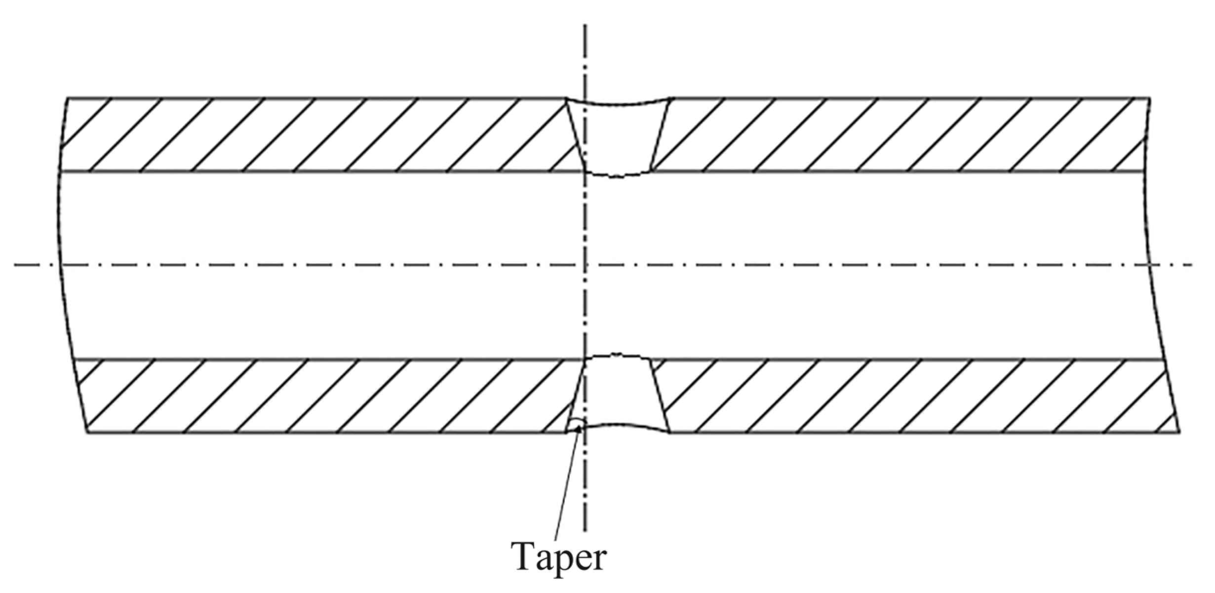
3. Optimized Design of Throttle Orifice Shape

Fluid control valves must have excellent throttling performance when adjusting each production segment of horizontal wells. The design of the throttle orifice needs to meet two necessary conditions. One is the throttle orifice meeting production demand under a specific differential pressure; another one is the need to have the most significant possible throttling differential pressure when the throttling area is unchanged.

There are three main traditional shapes of throttle orifices, as shown in Figure 3. Figure 3a is a rectangular throttle orifice; Figure 3b is a circular throttle orifice; and Figure 3c is an elliptical throttle orifice.

Under the premise of ensuring that the orifice overflow area is the same, the left and right sides of the rectangular throttle orifice are inclined along the inside to establish a trapezoidal throttle orifice, as shown in Figure 4. At the same time, the left and right sides of the rectangular throttle orifice are inclined along the outside to establish an inverted trapezoidal throttle orifice, as shown in Figure 5.

4. Evaluation of Trapezoidal Orifice Throttling Performance

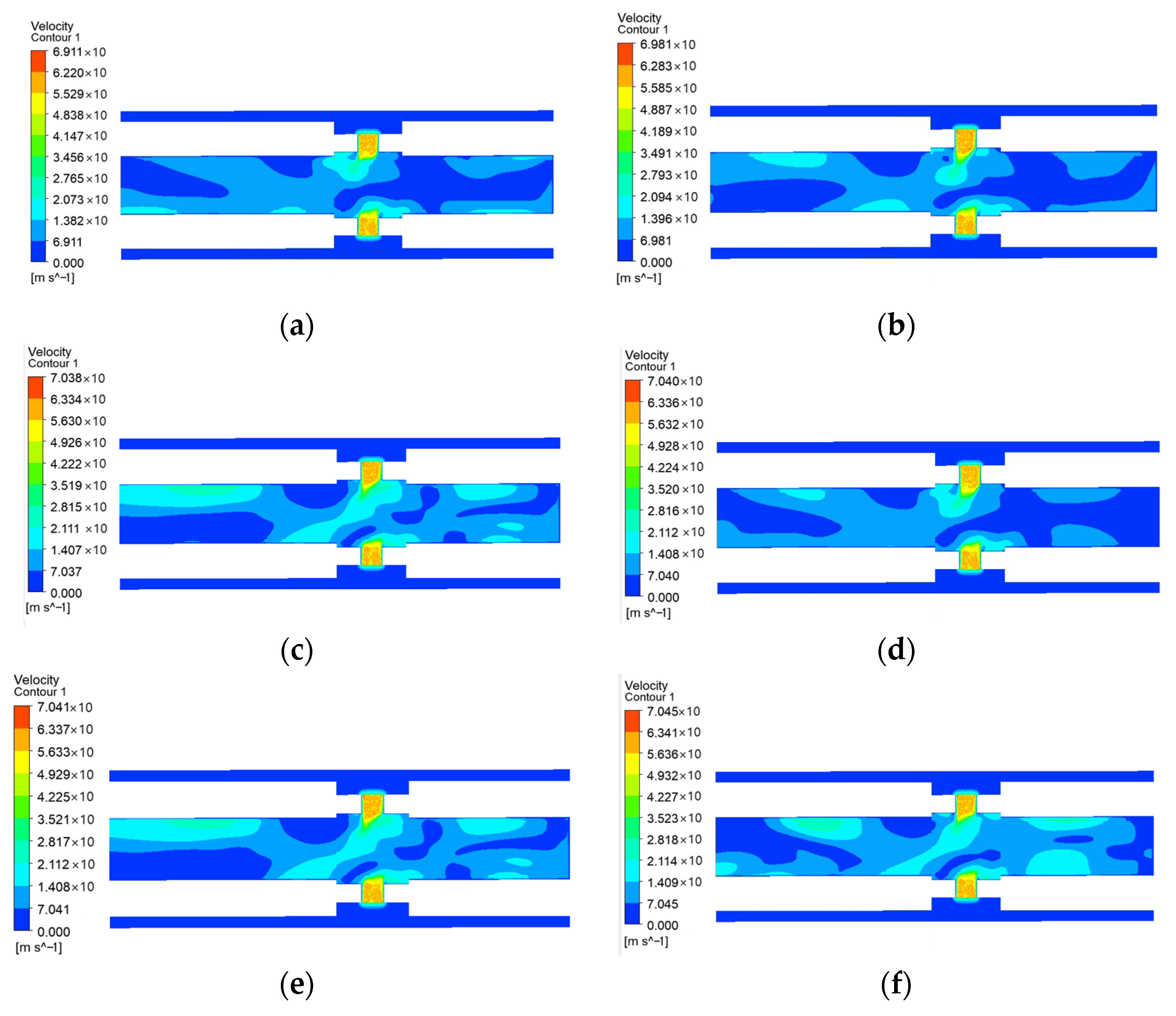
4.1. Grid Independence Test of Throttle Orifices

Grid independence must be verified first during the calculation process to ensure the correctness of simulation results. The flow rate and pressure model from another study [20] was used for numerical simulation. The calculation results are below for six grid schemes at 0.03 MPa differential pressure using the rectangular throttle orifice. The velocity diagrams for various numbers of grids are shown in Figure 6.

The results after extraction of the maximum flow velocity in each different grid number are shown in

Table 2. Calculated results for different numbers of grids.

Number of Grids	Maximum Flow Velocity (m/s)	Rate of Change
621,452	69.11	--
754,215	69.81	1.01%
885,456	70.38	0.82%
1,045,741	70.40	0.03%
1,202,101	70.41	0.01%
1,321,520	70.45	0.06%

.

As shown in Table 2, when the number of grids reaches 885,456 or more, the maximum flow rate change rates are 0.03%, 0.01%, and 0.06, respectively. The maximum flow rate change amplitude is minimal and almost tends to be stable. Therefore, this study selected a grid number of 885,456 for the numerical simulation. The grid independence was verified to meet the computational requirements.

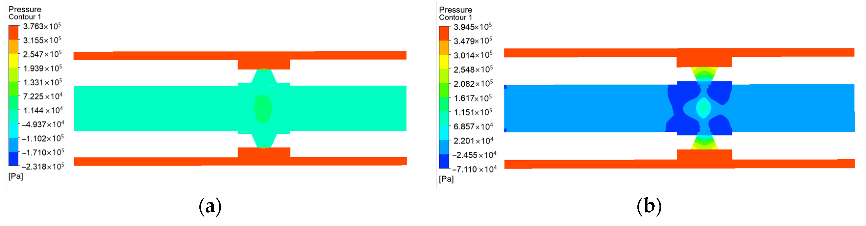
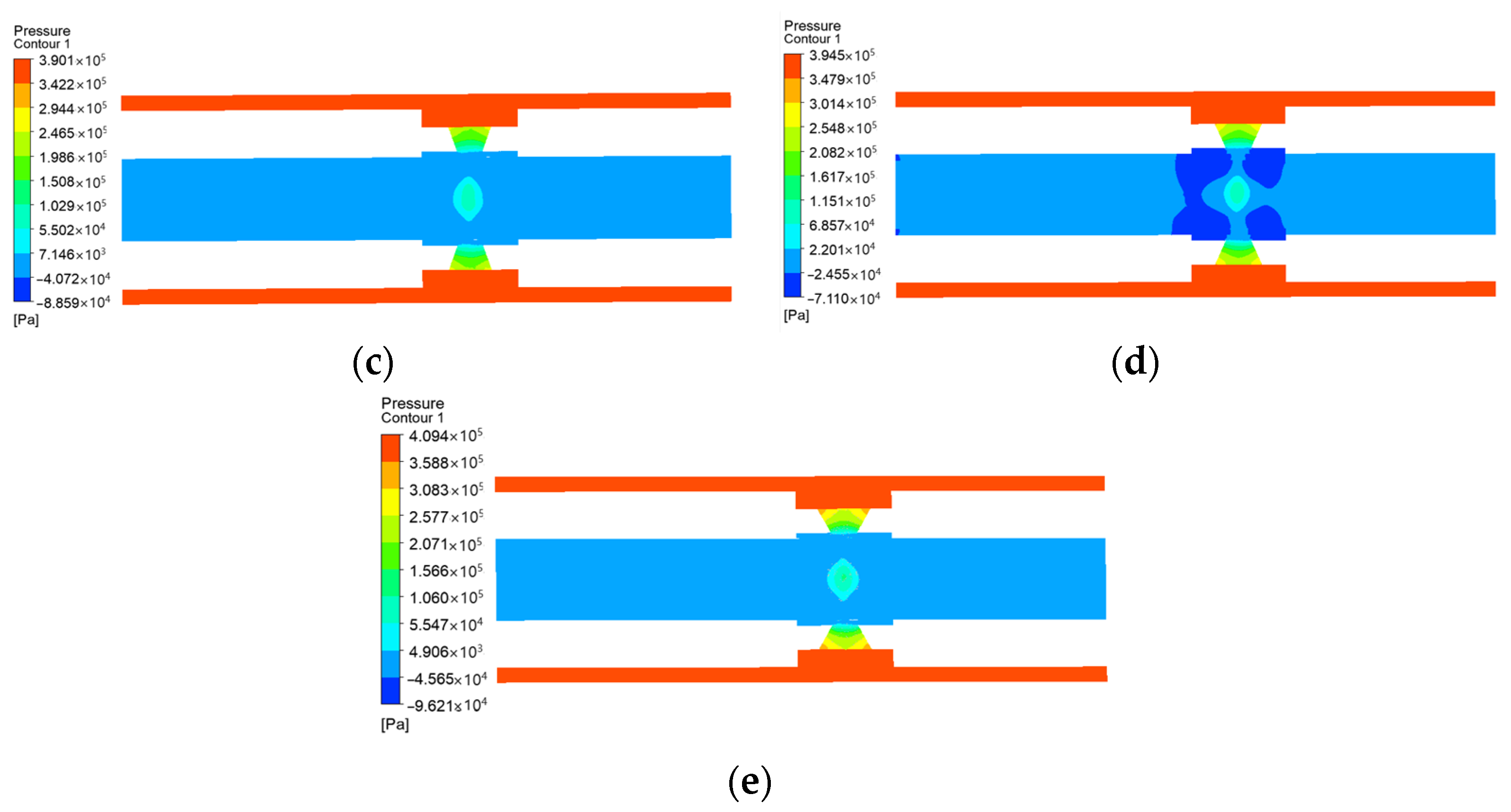
4.2. Comparison of Throttle Differential Pressure of Different Shapes of Throttle Orifices

The width of the throttle orifice was set to 5 mm and the length was set to 24 mm [12] to establish a rectangular throttle orifice. While ensuring the same throttle area, the two short sides of the rectangular throttle orifice were radially inclined by 25° to establish a trapezoidal throttle orifice and an inverted trapezoidal throttle orifice. Elliptical and circular orifices were created with the same throttle area. The differential pressure between the trapezoidal throttle orifice and the inverted trapezoidal throttle orifice was obtained, as shown in Figure 7.

The fluid pressures in the two diagrams in Figure 7 changed after the fluid passed through the throttle orifice. The gradient of pressure change was most evident in the trapezoidal throttle orifice. The differential pressure of the three conventional shapes of the throttle orifices was simulated using the same method. The results are summarized in

Table 3. Differential pressure of different orifices.

Shape	Differential Pressure (MPa)
Elliptic	0.261
Circular	0.291
Rectangular	0.332
Inverted trapezoid	0.376
Trapezoid	0.394

.

From the results of Table 3, when the throttle area was the same, the throttling differential pressure of the rectangular throttle orifice in the traditional shape throttle orifice was the largest. The maximum throttling differential pressure was 0.332 MPa. The maximum throttling differential pressure of the inverted trapezoidal throttle orifice was 0.376 MPa, which is 13.25% higher than that of the traditional rectangular throttle orifice. The maximum throttling differential pressure of the trapezoidal throttle orifice was 0.394 MPa, which is 18.6% higher than that of the traditional rectangular throttle orifice.

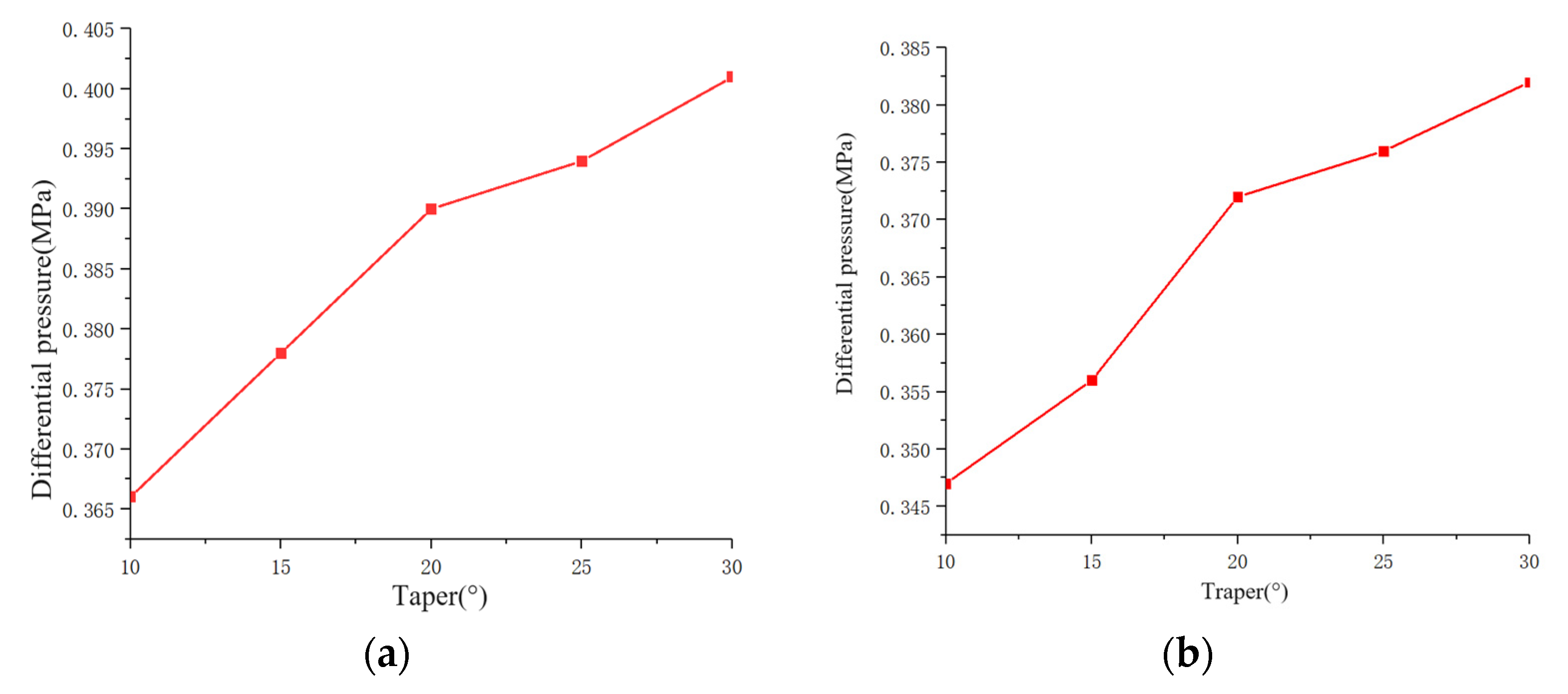
4.3. Effect of the Trapezoidal Throttle Orifice Taper on Differential Pressure

To further compare the effect of the taper of the trapezoidal and the inverted trapezoidal orifice on the throttling performance, the tapers were categorized as 10°, 15°, 20°, 15°, and 30°. Figure 8 shows the pressure diagram of the trapezoidal orifice at different tapers.

From Figure 8, the maximum pressure at the trapezoidal throttle orifice increases with the taper increase. Meanwhile, the pressure diagram of the inverted trapezoidal throttle orifice was simulated using the same method. The simulation results of the trapezoidal throttle orifice and inverted trapezoidal throttle orifice were made into curves, as shown in Figure 9.

As shown in Figure 9, the throttling differential pressure of the trapezoidal throttle orifice and the inverted trapezoidal throttle orifice increased with the taper increase. The reason is that with the taper increases, the difference between the outlet area and the inlet area of the throttle orifice becomes more extensive. Therefore, the differential pressure also increases. The maximum throttling differential pressure of 0.409 MPa for the trapezoidal throttle orifice is higher than that of 0.382 MPa for the inverted trapezoidal throttle orifice. To further compare the productivity of the two throttled orifices at different tapers, the differential pressure of natural gas in a horizontal well was assumed to be 0.03 MPa. The simulation results of its daily production of natural gas are shown in Figure 10.

From the results, the production of natural gas increases with the increase in the taper in both throttle orifices. The reason is that as the taper rises, the more significant the difference between the outlet area and the inlet area of the throttle orifice. This resulted in the greater differential pressure. As seen in Figure 10, the production of the trapezoidal throttle orifice increased from 11,976 m³/d to 12,374 m³/d, which is only about 3.3%. The production of the inverted trapezoidal throttle orifice increased from 9072 m³/d to 9398 m³/d, only about 3.6%. Overall, the effect of the change in the taper of the throttle orifice on the production was small and negligible. Therefore, the trapezoidal throttle orifice was selected for erosion research to ensure a considerable throttling differential pressure.

5. Effect of the Trapezoidal Throttle Orifice’s Taper on Erosion

When the fluid control valve is in working condition, the high-velocity particles hitting the wall surface of the throttle orifice will produce an obvious erosion phenomenon [29]. Solid particles on the wall erosion will form erosion pits after some time. Too large erosion pits will cause the seal failure of fluid control valves [30]. Therefore, it is significant to research the erosion effects of different tapers, sand contents, and particle sizes on the trapezoidal throttle orifice to find the best anti-erosion structure.

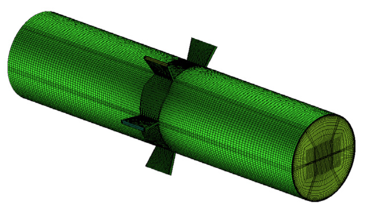
5.1. Erosion Calculation Domain Model

When establishing the erosion calculation domain model, to ensure the stable flow of the fluid through the throttle orifices into the flow channel, the length of the channel to the left and right was three times the diameter of the channel [31]. The taper of the throttle orifice was set to 0°, 5°, 10°, 15°, 20°, and 25°. The taper β is shown schematically in Figure 11. A grid of the model with different tapers was derived. Figure 12 shows the grid model with the 10° taper.

5.2. Erosion Boundary Conditions

The mouth of the throttle orifice was set as the velocity inlet, and the mouth of the pipe was set as the pressure outlet. The sand volume fractions were set to 2%, 3%, 4%, 5%, and 6%. The mass flow rates correspond to the volume fractions; other specific parameters are shown in

Table 4. Erosion parameters.

Working Medium	Taper (°)	Inlet Velocity (m/s)	Outlet Pressure (MPa)	Turbulence Intensity (%)		Hydraulic Diameter (mm)
				Inlet	Outlet	Inlet	Outlet
Natural gas	0	18	0	2.1	2.5	8.9	108
	5			2.1	2.5	8.9	108
	10			2.1	2.5	9.1	108
	15			2.2	2.5	9.18	108
	20			2.2	2.5	9.27	108
	25			2.2	2.5	9.34	108
Sand	Density (kg/m3)	Sand particle size (mm)	Mass flow rate (volume fraction) (kg/s)			Particle size function	Impact velocity function
	1550	0.05~0.75	0.005, 0.01, 0.015, 0.02, 0.025			4.2 × 10−9	1.73

.

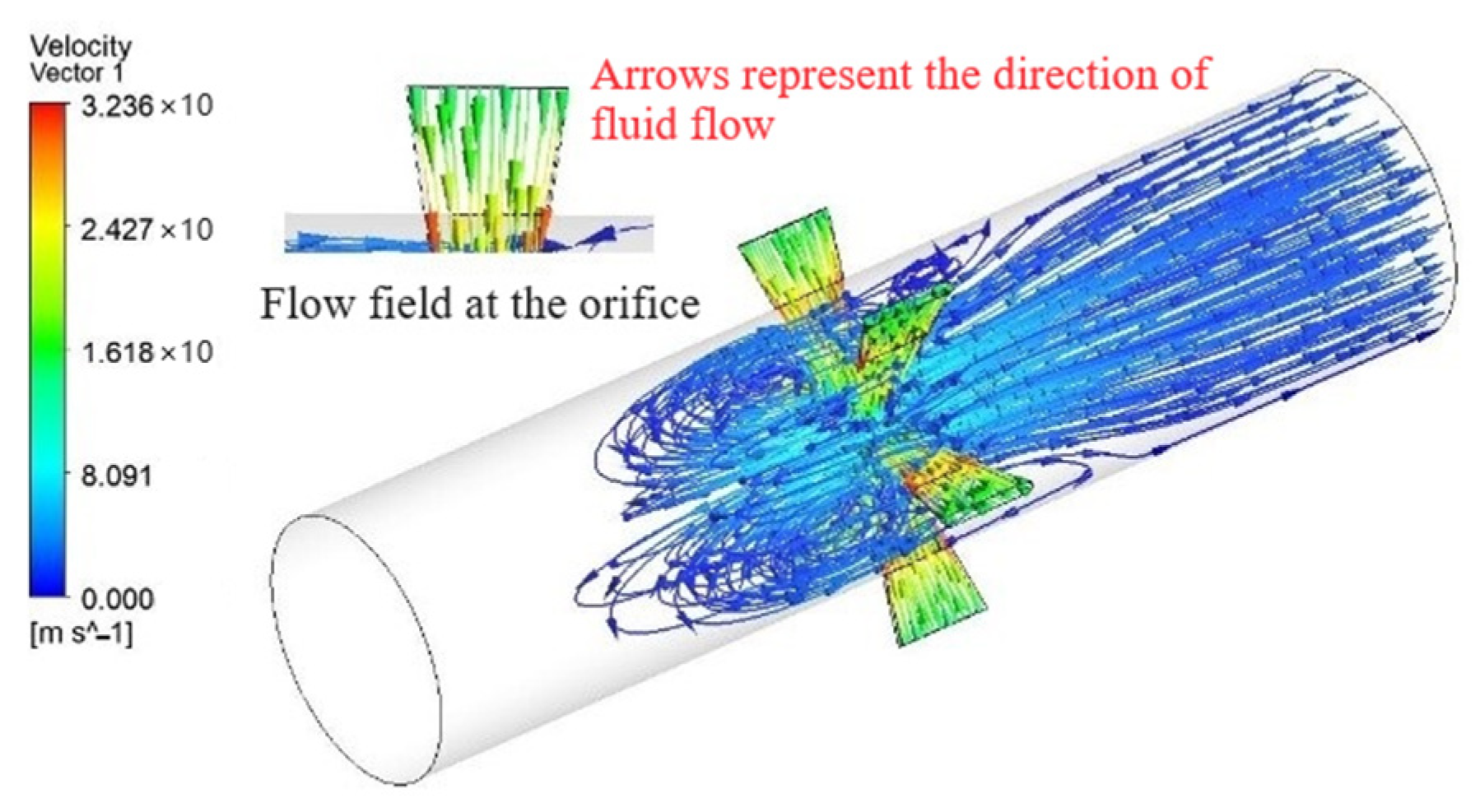
5.3. Flow Field Analysis

Velocity and pressure field diagrams were extracted for the 10° taper, as shown in Figure 13.

As shown in Figure 13, the velocity and pressure of natural gas as it passes through the throttle orifice changes with the changes in the dimensions and orientation of the cross-section of the channel. The higher pressure in the diagram corresponds to a lower velocity value. This is in line with the distribution characteristics of high pressure in the low-velocity region and low pressure in the high-velocity region, as reflected by Bernoulli’s equation. The extracted overall flow diagram is shown in Figure 14.

As shown in Figure 14, the flow velocity of natural gas is more significant at the left and right sides of the throttle orifice. In addition, it is significant at the junction of the throttle orifice and the inner channel. Therefore, it is assumed that the sand carried by the natural gas with a significant flow velocity will produce erosion and wear on the left and right sides of the throttle orifice.

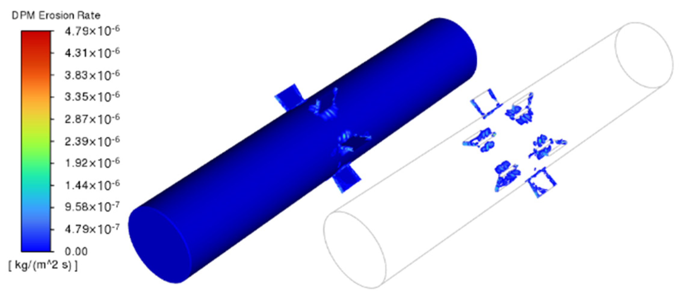
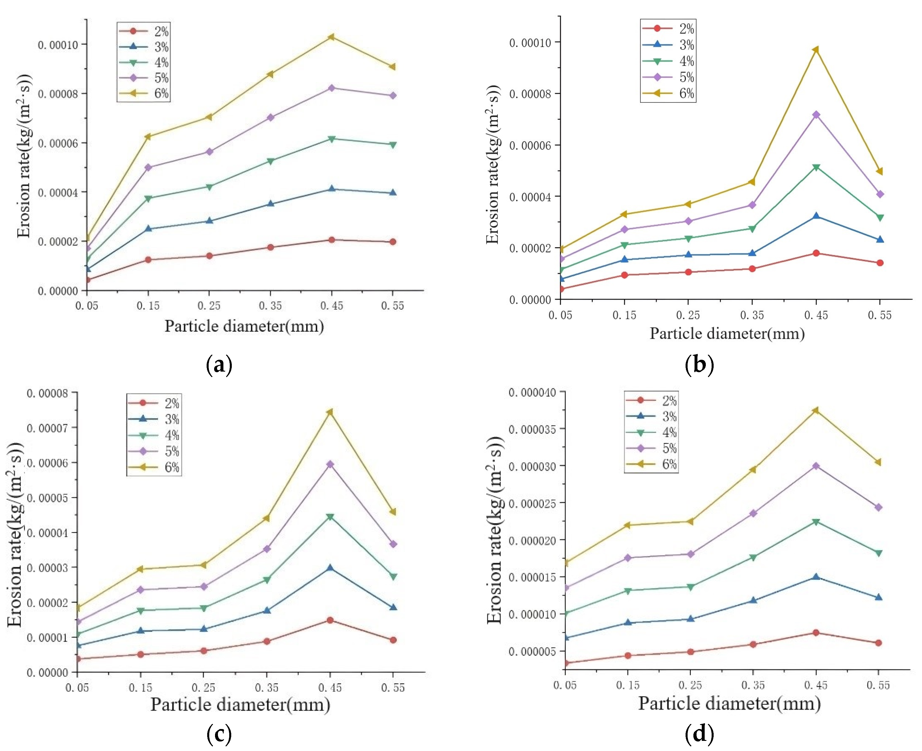
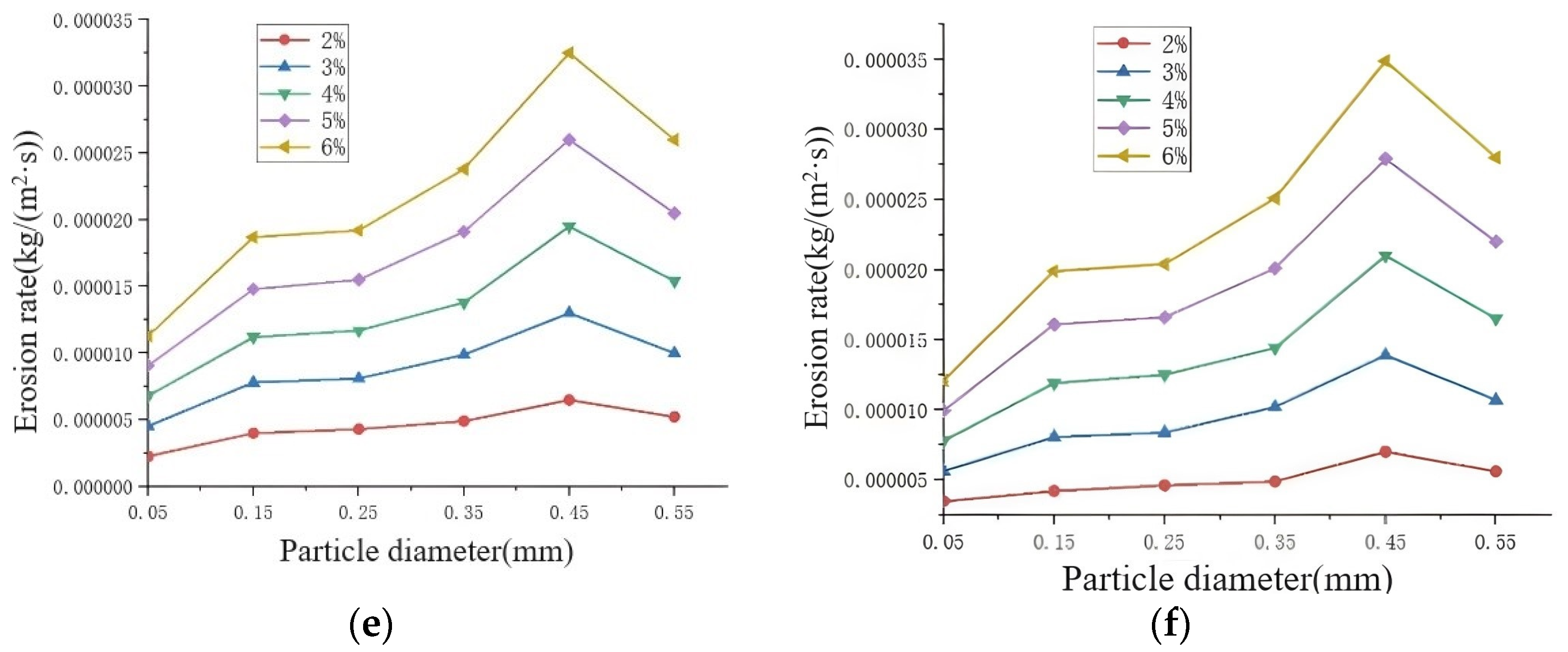
5.4. Analysis of Erosion Results

Figure 15 shows the distribution of the erosion for the throttle orifice with the 10° taper, the 6% sand volume fraction, and the particle size of 0.45 mm.

From Figure 15, the sand particles with high velocity impacted the left and right walls of the throttle orifice and the junction wall of the throttle orifice and the inner channel. The energy loss generated by the movement of particles is converted into erosive wear on the walls, which verifies the speculation in Figure 14.

Considering the effect of the opening of the throttle orifice on the erosion, the erosion for the same conditions with openings of 75%, 50%, and 25% is simulated as follows. The end with the reduced opening of the throttle orifice is considered a vertical wall surface.

As shown in Figure 16, the erosion still occurred mainly on the sloping surface of the side of the trapezoidal throttle orifice at different openings. When the opening was varied, almost no erosion occurred on the vertical wall at the side where the opening was reduced. The erosion rates at the four openings of the appeal were made into a line graph, as shown in Figure 17.

As shown in Figure 17, the erosion rate shows a wave-like change as the opening decreases. The opening decreases from 100% to 25%, and the erosion rate increases from 4.79 × 10⁻⁶ kg/(m²·s) to 6.6 × 10⁻⁶ kg/(m²·s), which is a small increase. The reason is that the decrease in the opening leads to a slight increase in the fluid velocity, leading to a slight increase in the erosion rate. Overall, the change in the erosion rate is minor when the opening is reduced. From the analytical results shown in Figure 16, erosion occurs mainly on the sloping surface of the side of the throttle orifice when the opening is changed. However, the change in the opening has a minor effect on erosion. Therefore, this study ignored the effect of the opening change on the erosion to facilitate the comparison and uses the 100% opening for numerical simulation.

All the results are gathered in Figure 18.

For the variation in the curves in Figure 18:

(1)

For throttle orifices with different tapers, the erosion rate shows a trend of increasing and decreasing with the particle diameter increase.

(2)

The erosion rate changes slowly in the particle diameter interval of 0.05–0.25 mm. As in Figure 16c, the erosion rate of 6% sand content increased by 66.7%. The reason is that at smaller particle diameters, the particles have less mass and are more affected by the turbulence intensity of the fluid. Therefore, the particles follow the fluid movement more strongly and hit the wall less often.

(3)

In the particle diameter interval of 0.25–0.45 mm, the growth of the erosion rate is accelerated. For example, in Figure 16c, the erosion rate of 6% sand content increased by 146.7%. The reason is that the kinetic energy also gradually increases with the gradual increase in the mass of the particles. As the kinetic energy of the impact of the particles on the wall increases, the resulting erosion pits gradually increase.

(4)

As the size of the particle increases further (>0.45 mm), the mass of the particle becomes non-negligible. The reduced fluid following of the large mass of particles affects the kinetic energy, and the erosion rate decreases. All the throttle orifices with different tapers are subjected to maximum erosion at a sand particle diameter of 0.45 mm.

Figure 19 shows a line graph plot of the variation in the erosion rate of the six groups of the throttle orifices at different sand contents, with a sand particle diameter of 0.45 mm.

As seen in Figure 19, at the same particle diameter and the taper, the erosion rate shows a linear increase with the increase in sand content. The reason is that the larger the sand content, the more erosion of the throttle orifice plate per unit of time, and the greater the erosion rate. The erosion rate is minimized at a taper of 20°. The reason is that when the taper is 0°, the sand particles are equivalent to the incident at 90°. Therefore, the sand particles impact the junction wall of the throttle orifices and the inner channel and cause the most severe erosion of the place. When the taper increases, the particle incident direction and the pipe wall angle decrease. Thus, the wall erosion gradually decreases. When the taper exceeds 20°, the sand particles are equivalently incident at a large angle of impact on the wall of the throttle orifice. Thus, the wall erosion increases.

Figure 20 shows the variation curves of the maximum erosion rate for different tapers of throttle orifice.

At all sand volume fractions, the maximum erosion rate first decreased and then increased with the increasing taper. Finally, the minimum erosion rate was achieved at 20° taper. For example, the maximum erosion rate decreased from 0.00013 kg/(m²·s) to 0.000034 kg/(m²·s) at 6% sand content.

6. Discussion

Further research at the 20° taper was performed; the results are shown below.

As shown in Figure 21, the erosion rate first decreased and then increased as the taper increased. The erosion rate decreased as the taper increased from 20° to 21°. When the taper exceeded 21°, the erosion rate gradually increased.

A throttle orifice taper that is too large will produce considerable erosion, while a taper that is too small will lower the throttling differential pressure. Meanwhile, it is difficult to machine throttle orifices with a precise taper in actual engineering. Therefore, the throttle orifice taper is best at about 20°.

Due to fracturing work, much research has been carried out on the erosion of the orifice of sliding sleeve-type valves, such as fluid control valves [22]. However, research on the throttling performance and anti-erosion structure of new throttle orifices of fluid control valves has yet to be reported. In other studies of similar sliding sleeve-type valves, designing for throttle orifices and increasing the inclination of orifices has been researched, with proven excellent results. For example, Kou et al. [32] examined the erosion-influencing factors of sliding sleeve-type blowdown valves. Moreover, the throttle orifice was designed to be inclined. However, the study only considered the effect of the change in the opening on the erosion rate; it ignored the inclination angle, which is the main influencing factor. Research on the impact of the inclination angle of the throttle orifice on erosion is an essential indicator for the throttle orifice design.

In fact, better throttling performance of the throttle orifice may lead to increased erosion to a certain extent [33]. In the future, intelligent adjustment of the size of the throttle orifice will be an essential research direction [34]. However, balancing the different throttling effects and erosion aggravation brought by the change in the size of the throttle orifice is an important issue. Therefore, designing a novel shape of the throttle orifice to solve the above problems can be an essential method.

7. Conclusions

• For the same throttle area, the differential pressure of the trapezoidal orifice is about 18.6% higher than that of the traditional rectangular orifice. The result proves that the trapezoidal orifice has excellent throttling performance.
• The throttling differential pressure of the trapezoidal throttle orifice increases with the increase in the taper. When the taper increases from 10° to 30°, the differential pressure increases from 0.347 MPa to 0.409 MPa. For a differential pressure of 0.03 MPa, the production of natural gas increases with the taper. When the taper is increased from 10° to 30°, the production of natural gas increases from 11,976 m³/d to 12,374 m³/d, an increase of only about 3.3%. Overall, the effect of the change in the taper on gas production is small and negligible.
• When the particle size is 0.45 mm, the trapezoidal throttle orifice is subjected to maximum erosion. In the 0 to 25° taper, the maximum erosion is the first to decrease and then increase as the taper increases. The minimum erosion rate is achieved at about 20°. The above research methods can provide a theoretical basis for optimizing the size and structure of orifices and sealing the reliability of fluid control valves.

References

1. Tan, L.; Xie, L.; He, B.; Zhang, Y. Multi-Fracture Propagation Considering Perforation Erosion with Respect to Multi-Stage Fracturing in Shale Reservoirs. Energies 2024, 17, 828. [Google Scholar] [CrossRef]
2. Li, T.; Zhang, J.F.; Guan, Y.Z. Research Progress of Capacity Evaluation Techniques for Horizontal Well Segmental Fracturing in Various Segments. Sci. Technol. Eng. 2023, 23, 8916–8927. [Google Scholar]
3. Yuan, J. New Progress and Development Suggestions of SINOPEC’s Horizontal Well Drilling Technology for Ultra-Long Horizontal Segments of Shale Gas. Pet. Drill. Tech. 2023, 51, 81–87. [Google Scholar]
4. Cui, X.J.; Li, H.T.; Li, S.X.; Li, Y.F.; Ge, J.R.; Wang, N. Integrated Intelligent Completion Technology for Water Searching and Control in Horizontal Wells and Its Application. China Offshore Oil Gas. 2021, 33, 158–164. [Google Scholar]
5. Eren, T.; Polat, C. Numerical investigation of the application of intelligent horizontal well completion. J. Nat. Gas. Sci. Eng. 2020, 83, 103599. [Google Scholar] [CrossRef]
6. Li, R.F.; Zhang, L.; Liu, J.C.; Yang, J.Y. Research on Ground Control System of Intelligent Completion Technology. Shipbuild. China 2019, 60, 426–433. [Google Scholar]
7. Zhang, M.F. Discussion on the development status and trend of intelligent completion technology. Mod. Chem. Res. 2017, 10, 14–15. [Google Scholar]
8. Yang, Z.; Yang, J.; Wang, Q.; Sun, F.J. Research and Application of Plunger Airlift Draining Gas Recovery Intelligent Control Technology in Shale Gas Horizontal Wells. Chem. Technol. Fuels Oils 2022, 58, 554–560. [Google Scholar] [CrossRef]
9. Giden, I.; Nirtl, M.; Maier, H.T.; Ismail, I.M. Horizontal infill well with AICDs improves production in a mature field—A case study. In Proceedings of the SPE Europec featured at 81st EAGE Conference and Exhibition, London, UK, 3–6 June 2019; pp. 85–90. [Google Scholar]
10. Muradov, K.; Eltaher, E.; Davies, D. Reservoir simulator-friendly model of fluid-selective, downhole flow control completion performance. J. Pet. Sci. Eng. 2018, 164, 140–154. [Google Scholar] [CrossRef]
11. Muradov, K.; Haghighat Sefat, M.; Moradi Dowlatabad, M. Fast optimization of packer locations in wells with flow control completions. J. Pet. Sci. Eng. 2021, 205, 108933. [Google Scholar] [CrossRef]
12. Guo, D. Parametric Design and Analysis of Intelligent Downhole Flow Controller; Southwest Petroleum University: Chengdu, China, 2018. [Google Scholar]
13. He, M.G.; Ma, F.M.; Lin, L.J.; Yin, G.F. Design of downhole smart throttler and flow field analysis of throttling valve. China Pet. Mach. 2013, 41, 85–89. [Google Scholar]
14. Yang, Y.W.; He, D.S.; Xu, L.B.; He, Y.; Ye, Z.; Zheng, Y. Numerical Study on Flow Field Characteristics of Interval control valve in Intelligent Well. IOP Conf. Ser. Mater. Sci. Eng. 2019, 677, 42082. [Google Scholar] [CrossRef]
15. Li, C.; He, D.S.; Yang, Y.W.; Xie, X.L.; Dai, H. Research on flow channel of downhole flow control valve based on Fluent. Pet. Mechanical. 2022, 50, 78–85. [Google Scholar]
16. Zhou, J.H.; Zhang, Y.; Xiong, Z.Y.; Shang, J. Numerical simulation of throttling effect of throttling valves at the bottom of coalbed methane wells. J. China Univ. Pet. 2021, 45, 144–151. [Google Scholar]
17. Li, C.H. Adaptability Evaluation of Horizontal Well Inflow Control Valve (ICD) Completion Technology; Northeast Petroleum University: Daqing, China, 2016. [Google Scholar]
18. Chen, S.S.; Shi, P.Z.; Feng, Y.; Gai, J.A.; Lou, Y.S.; Di, X.P.; Shi, B.C. Prediction of erosion life of metal grid screen at different flow rates. China Pet. Mach. 2021, 49, 77–82. [Google Scholar]
19. Zhao, J.G.; Wang, J.; Han, S.; Sahmani, S.; Safaei, F. Probabilistic-based nonlinear stability analysis of randomly reinforced microshells under combined axial-lateral load using gridfree strain gradient formulations. Eng. Struct. 2022, 262, 1–25. [Google Scholar] [CrossRef]
20. Zhao, J.; Zheng, H.; Xie, C.; Xiao, X.; Han, S.; Huang, B.; Zhang, X. Research on the influence mechanism of fluid control valve on the production of segmented horizontal wells and the balanced gas production control model: A case analysis of Sichuan basin natural gas. Energy 2024, 294, 130837. [Google Scholar] [CrossRef]
21. Carloni, A.C.N.; de Conde, K.E.; Pantaleão, A.V.; de Azevedo, J.L.F.; Rade, D.A. Validation and analysis of turbulence modeling in pipe elbow under secondary flow conditions. J. Braz. Soc. Mech. Sci. Eng. 2022, 44, 595. [Google Scholar] [CrossRef]
22. Zhao, J.G.; Zheng, H.T.; Zeng, J.; Wang, G.R. Life prediction model of fracturing sliding sleeve based on Sichuan shale gas in China. Pet. Sci. Technol. 2023, 1–23. [Google Scholar] [CrossRef]
23. Lian, Z.H.; Chen, X.H.; Lin, T.J.; Zhang, X.K. Study on erosion mechanism of sand discharge pipeline elbow joints. J. Southwest. Pet. Univ. 2014, 36, 150–156. [Google Scholar]
24. Wang, W.; Sun, Y.; Wang, B.; Dong, M.; Chen, Y. CFD-Based Erosion and Corrosion Modeling of a Pipeline with CO2-Containing Gas–Water Two-Phase Flow. Energies 2022, 15, 1694. [Google Scholar] [CrossRef]
25. Zhang, Z.; An, C.; Wei, D.F.; Wang, Z.G. Numerical simulation study on sand erosion of underwater throttling valve. Ocean. Eng. 2022, 40, 160–172. [Google Scholar]
26. Edwards, J.K.; Mclaury, B.S.; Shirazi, S.A. Evaluation of alternative pipe bend fittings in erosive service. In Proceedings of the 2000 ASME Fluids Engineering Division Summer Meeting: Presented at the 2000 ASME FluidS Engineering Division Summer Meeting, Boston, MA, USA, 11–15 June 2000; American Society of Mechanical Engineers: New York, NY, USA, 2000. [Google Scholar]
27. Wang, K.; Li, X.F.; Wang, Y.S.; Chen, Y.L.; Han, S.; He, R.Y. Prediction of the location of solid particles in liquid-solid two-phase flow on the erosion damage of a pipe bend. J. Eng. Thermophys. 2014, 35, 691–694. [Google Scholar]
28. Grant, G.; Tabakoff, W. Erosion Prediction in Turbomachinery Resulting from Environmental Solid Particles. J. Aircr. 1975, 12, 471–478. [Google Scholar] [CrossRef]
29. Li, B.; Zeng, M.; Wang, Q. Numerical Simulation of Erosion Wear for Continuous Elbows in Different Directions. Energies 2022, 15, 1901. [Google Scholar] [CrossRef]
30. Zeng, J.; Zhu, H.Y.; Zhang, W.; Zheng, W.; Yang, Y.Q. Three-layer casing slip-on design and its erosion law analysis. Mach. Des. Res. 2018, 34, 181–186. [Google Scholar]
31. Frosell, T.; Mcgregor, M.; Ross, C. A comparison of proppant erosion during slurry injection. Can. J. Political Sci. 2014, 43, 770–773. [Google Scholar]
32. Kou, B.; Liu, E.; Li, D.; Qiao, W.; Chen, R.; Peng, S. Research on Erosion Characteristics of the Sleeve-Type Blowdown Valve in the Shale Gas Gathering and Transportation Station. SPE J. 2024, 29, 328–345. [Google Scholar] [CrossRef]
33. Liu, P.; Wang, C. Selection and Optimization of Throttling Process for Ultra-high Pressure Gas Wells. J. Southwest. Pet. Univ. 2023, 45, 145–154. [Google Scholar]
34. Zheng, J.; Li, J.; Wu, J.; Li, Z.; Zhang, Y. Review of Downhole Throttle Failure in Oil and Gas Wells. J. Fail. Anal. Prev. 2023, 23, 609–621. [Google Scholar] [CrossRef]
Figure 1. Schematic of the three-dimensional structure of the fluid control valve. 1—male connector; 2—electric control section; 3—optical fiber measurement section; 4—oil tank; 5—hydraulic power source; 6—hydraulic power section; 7—outer cylinder; 8—sliding sleeve; 9—inner cylinder; 10—female connector; 11—throttle orifice; 12—overflow orifice; 13—fracture orifice.
Energies 17 03196 g001
Figure 2. Schematic diagram of parameter directions.
Energies 17 03196 g002
Figure 3. Traditional throttle orifices: (a) rectangular; (b) circular; (c) elliptic.
Energies 17 03196 g003
Figure 4. Trapezoidal orifice diagram.
Energies 17 03196 g004
Figure 5. Inverted trapezoidal orifice diagram.
Energies 17 03196 g005
Figure 6. The velocity diagrams for different numbers of grids: (a) grid number 621,452; (b) grid number 754,215; (c) grid number 885,456; (d) grid number 1,045,741; (e) grid number 1,202,101; (f) grid number 1,321,520.
Energies 17 03196 g006
Figure 7. Different throttle orifice pressure diagram: (a) inverted trapezoid; (b) trapezoid.
Energies 17 03196 g007
Figure 8. Pressure diagram at different tapers of the throttle orifice: (a) 10° taper; (b) 15° taper; (c) 20° taper; (d) 25° taper; (e) 30° taper.
Energies 17 03196 g008aEnergies 17 03196 g008b
Figure 9. Effect of the taper on throttling differential pressure: (a) trapezoid; (b) inverted trapezoid.
Energies 17 03196 g009
Figure 10. Effect of the taper on the daily production of natural gas: (a) trapezoid; (b) inverted trapezoid.
Energies 17 03196 g010
Figure 11. Taper β diagram.
Energies 17 03196 g011
Figure 12. Erosion grid model with the 10° taper.
Energies 17 03196 g012
Figure 13. Velocity and pressure field diagram of the 10° taper. (a) velocity field. (b) Pressure field.
Energies 17 03196 g013
Figure 14. Overall flow diagram.
Energies 17 03196 g014
Figure 15. Erosion distribution diagram.
Energies 17 03196 g015
Figure 16. Erosion distribution diagram for different openings: (a) 75% opening; (b) 50% opening; (c) 25% opening.
Energies 17 03196 g016
Figure 17. Erosion rate for different openings.
Energies 17 03196 g017
Figure 18. Erosion rate for different tapers: (a) 0° taper; (b) 5° taper; (c) 10° taper; (d) 15° taper; (e) 10° taper; (f) 15° taper.
Energies 17 03196 g018aEnergies 17 03196 g018b
Figure 19. The change in the erosion rate with a sand particle diameter of 0.45 mm.
Energies 17 03196 g019
Figure 20. The maximum erosion rate for different tapers.
Energies 17 03196 g020
Figure 21. Refined erosion rate curve at the 20° taper.
Energies 17 03196 g021