
Thermal Analysis of Power Transformer Using 2D and 3D Finite Element Method

Abstract
1. Introduction
2. Methodology
- Model Creation
- Iron core: The central part of the transformer that guides the magnetic flux.
- High-voltage windings: Copper windings designed to handle high voltage.
- Low-voltage windings: Copper windings designed to handle low voltage.
- Insulating oil: Used for cooling and insulation within the transformer.
- External tank: The enclosure that contains the core, windings, and oil.
- Rating: 300 MVA
- Voltage: 16.5/240 KV
- Configuration: ∆/Y (Delta/Star)
- Phase: Three-phase unit
- Location: Kureimat Station, Egypt
- Application: Combined cycle power plant
- Core losses: Heat generated due to hysteresis and eddy currents in the core.
- Winding losses: Heat generated due to the resistance in the copper windings.
- Operational losses: Additional heat generated during the operation of the transformer.
- Heat generated within the transformer is dissipated to the ambient air.
- The dissipation process occurs in multiple stages, driven by temperature differentials at each boundary.
- Model Analysis
- Calculate the losses occurring within the transformer.
- Input these loss values into the 2D and 3D FEM models.
- Use the models to analyze the temperature distribution within the transformer under different load conditions.
- Compare the temperature distribution results obtained from the FEM analysis with actual temperature measurements.
- Use the test report from Hyundai to verify the accuracy of the FEM model predictions.
Geometry Description
3. Finite Element Method
Governing Equations
- T temperature (K)
- x, y, and z spatial variables (m)
- K thermal conductivity (W/m·K)
- q′ heat transfer rate (W/m3)
- ρ density (Kg/m3)
- C specific heat (J/kg·K)
- t time (s)
4. Heat Flow and Boundary Conditions
4.1. Convection
4.1.1. Free Convection
4.1.2. Forced Convection
4.2. Radiation
5. Transformer Losses
5.1. Iron Losses (PNL)
5.2. Load Losses (PLL)
5.2.1. Ohmic Losses (PR)
5.2.2. Winding Stray Loss (PEC)
- PEC−r rated eddy current losses, W
- K load coefficient with respect to the rated load value
- I1−r primary rated current, A.
5.2.3. Other Stray Loss (POSL)
5.2.4. Total Stray Losses (PTSL)
5.3. Dielectric Losses (PD)
6. Simulation and Results
6.1. Power Transformer Simulation Model
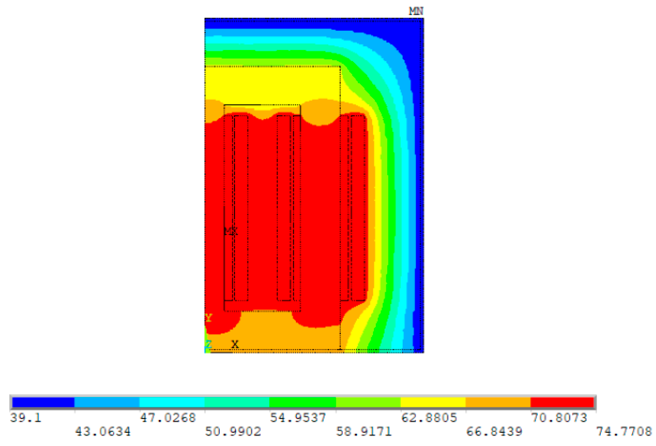
6.1.1. 2D Modelling
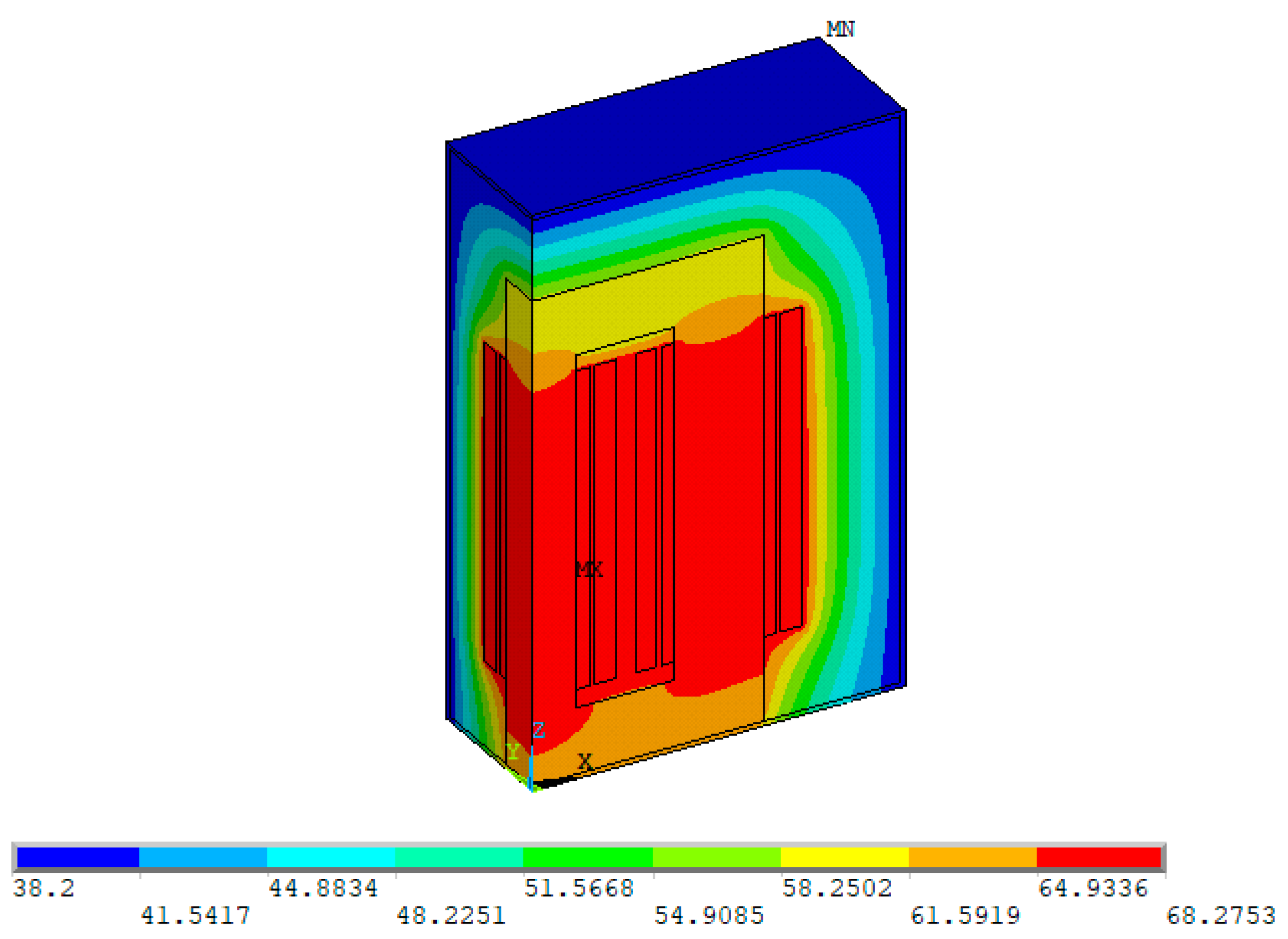
6.1.2. 3D Modelling
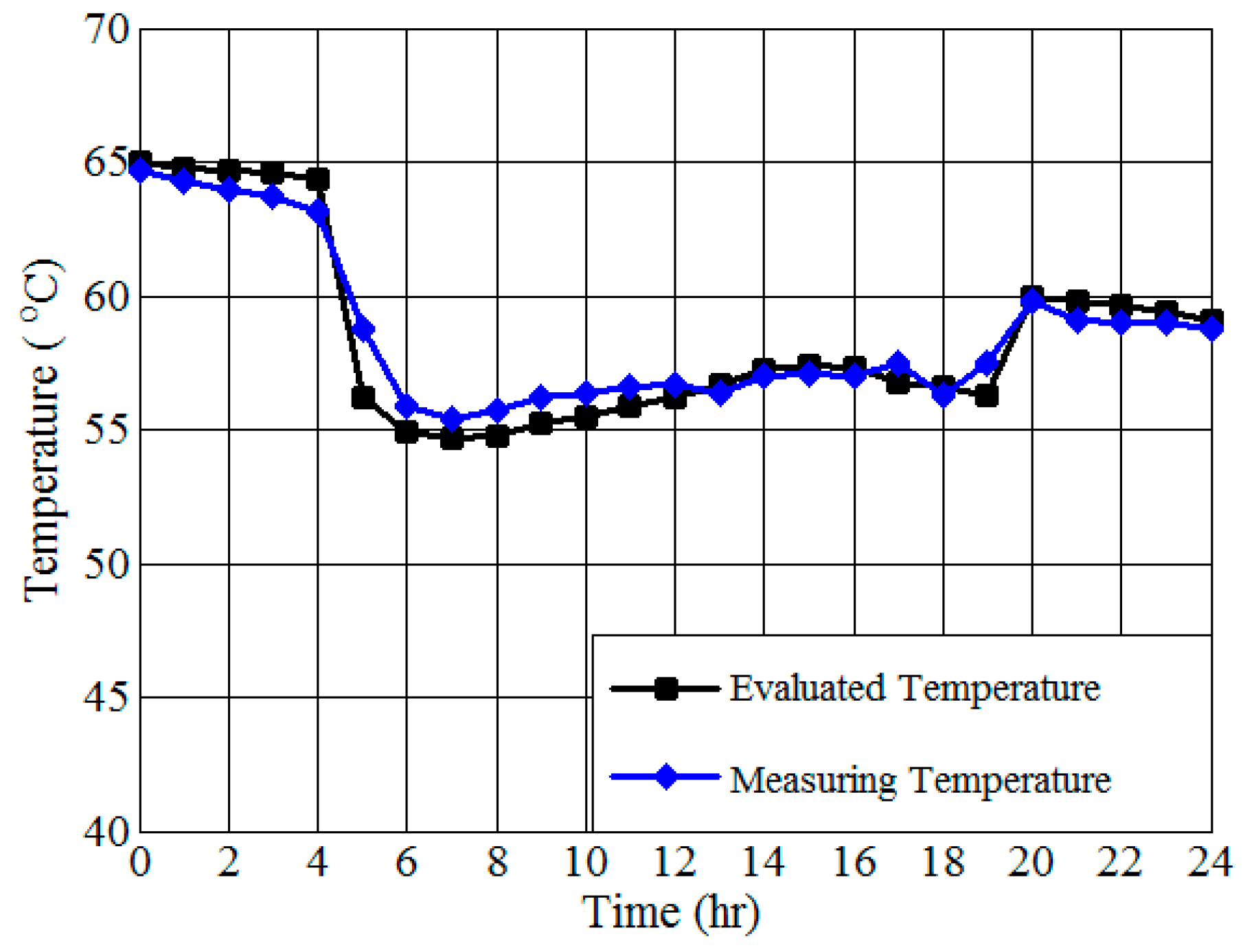
6.2. Transient Performance for Oil-Immersed Transformer
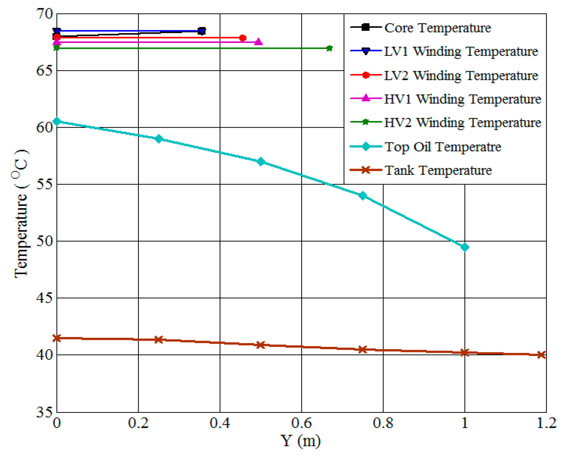
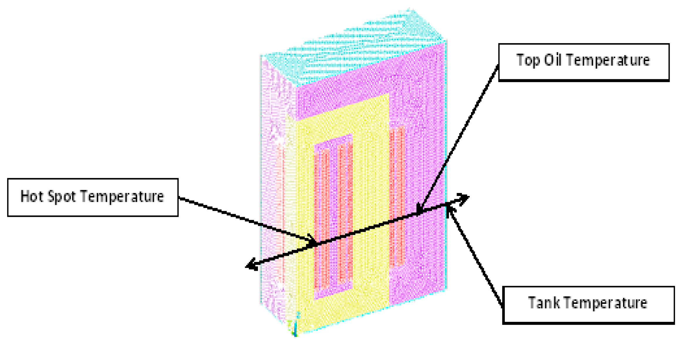
6.3. Thermal Performance of the Transformer under Different Conditions
6.3.1. Different Oil Viscosities
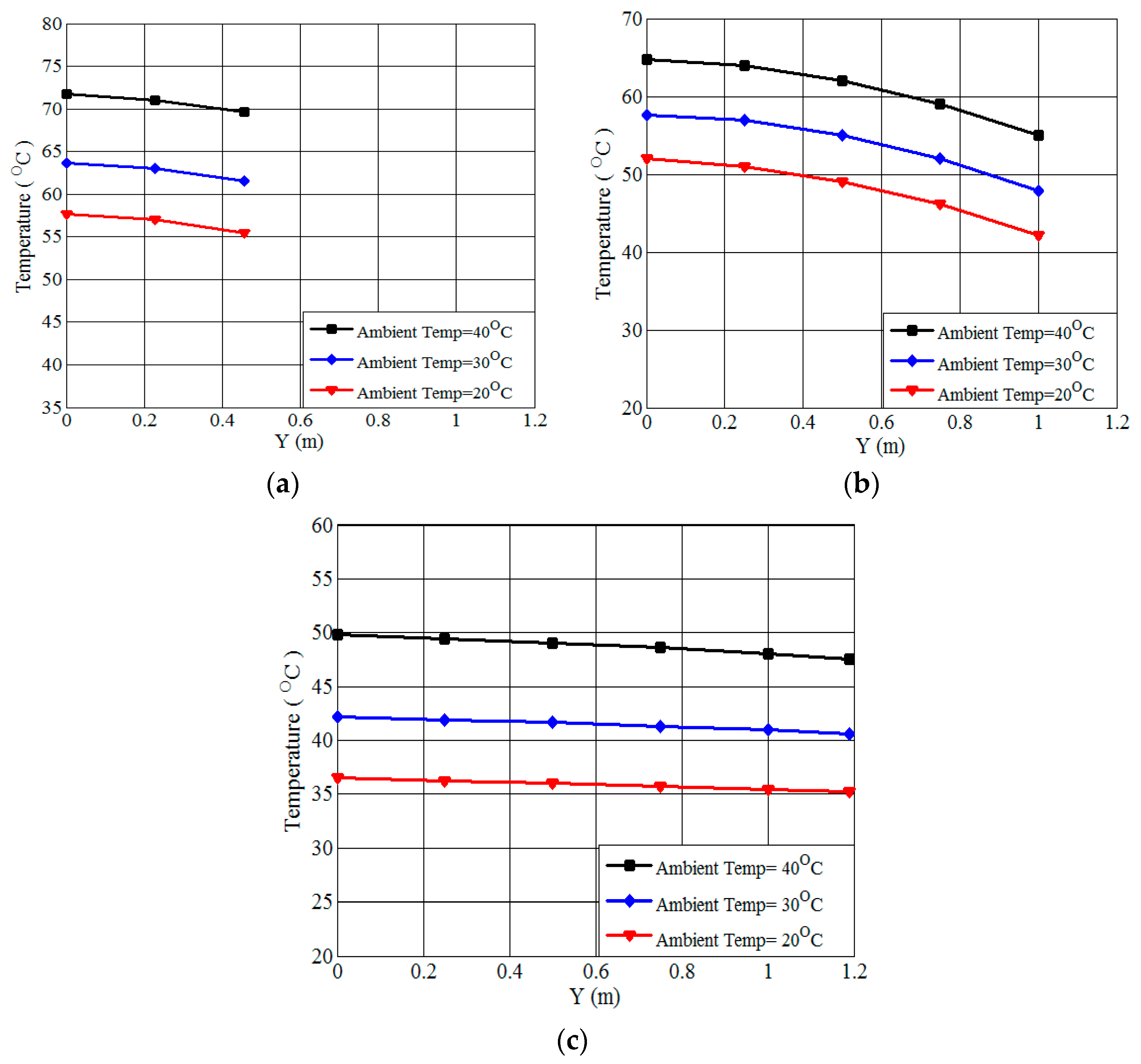
6.3.2. Ambient Temperature
6.3.3. Effect of Cooling Modes (ONAN/ONAF1/ONAF2)
- ONAN (Oil Natural Air Natural):
- ONAF1 (Oil Natural Air Forced Stage 1):
- ONAF2 (Oil Natural Air Forced Stage 2):
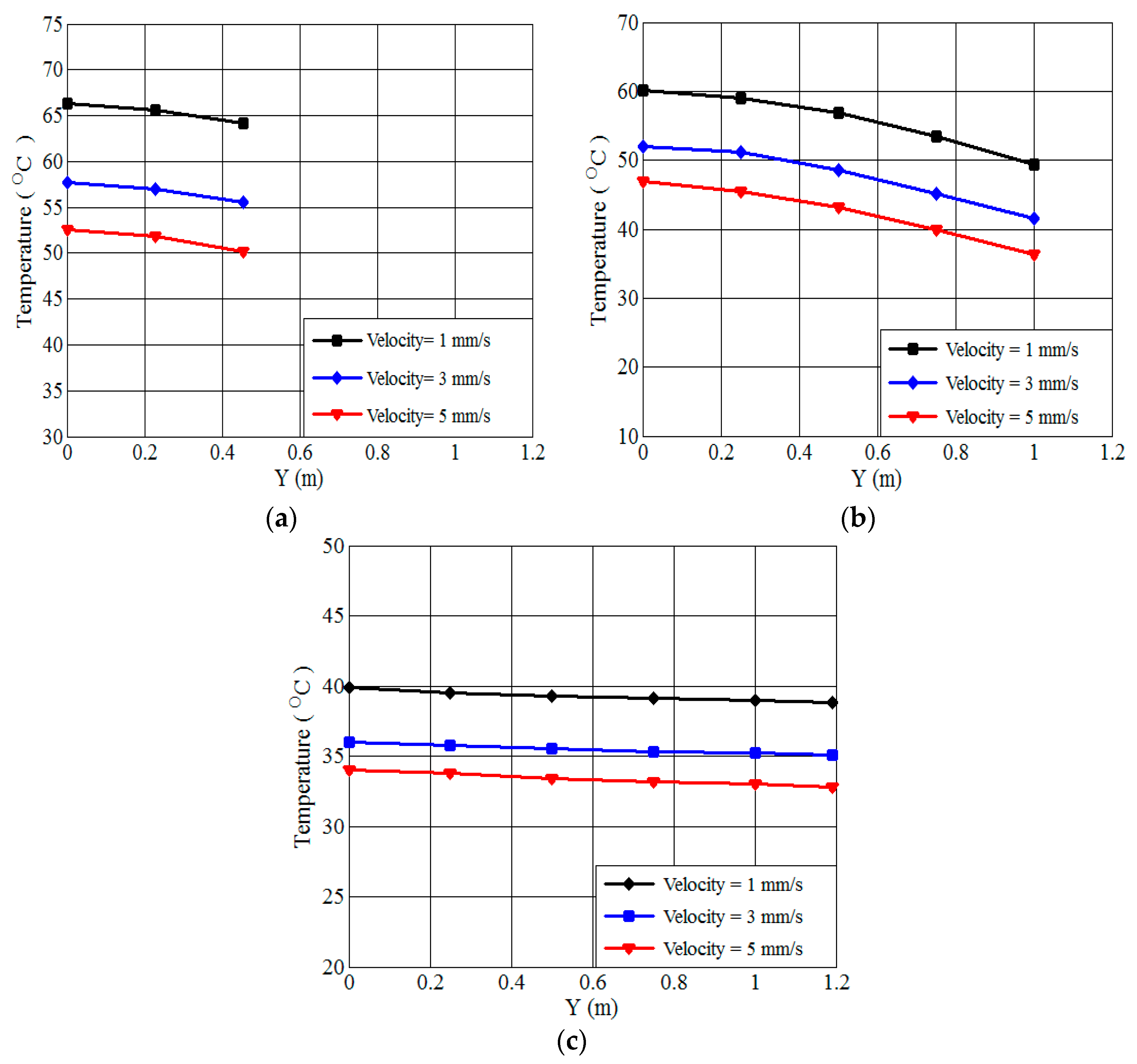
6.3.4. Effect of Oil Velocity
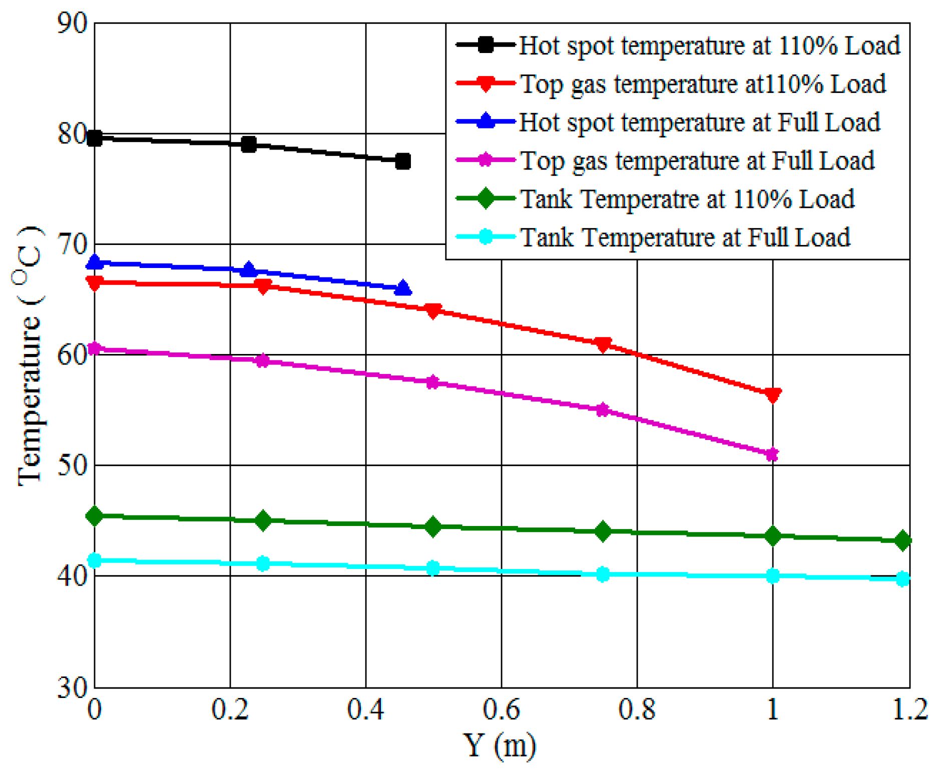
6.3.5. Overloading the Transformer
6.3.6. Changing the Fluid with SF6
7. Conclusions
- The impact of oil viscosity on component temperatures, where a 1 mm3/s viscosity increase leads to a 3 °C temperature increase, highlighting lower-viscosity oils for better cooling.
- Ambient temperature variations from 20 to 40 °C affect the 3D oil-immersed transformer model’s behavior at 240 MVA, demonstrating noticeable effects.
- Different cooling modes (ONAN/ONAF1/ONAF2) at 80% load and 20.6 °C ambient temperature reveal significant impacts on transformer component temperatures, with forced cooling showing a pronounced effect.
- Oil velocity’s influence on temperature distribution is analyzed, showing that higher oil velocities enhance cooling and reduce transformer temperatures.
- Overloading the transformer at 110% load is investigated, comparing computed temperatures with maximum load model outputs.
- A 3D model comparison between SF6 and oil-immersed transformers under load cycles and varying ambient conditions shows SF6’s superior performance in certain scenarios.
Author Contributions
Funding
Conflicts of Interest
References
- Prytkov, S.F.; Gorbachev, V.M. Handbook Reliability of Radioelements; Moscow, Russia, 2012. [Google Scholar]
- Susa, D.; Lehtonen, M. Dynamic Thermal Modeling of Power Transformers: Further Development—Part I. IEEE Trans. Power Deliv. 2006, 21, 1961–1970. [Google Scholar] [CrossRef]
- AValuyskih, O.; Dulkin, I.N.; Filippov, A.A.; Tsfasman, G.M. Modeling of the thermal regime of the transformer in the control, monitoring and diagnostics. Electro 2008, 1, 15–19. [Google Scholar]
- Jahromi, A.; Piercy, R.; Cress, S.; Service, J.; Fan, W. An approach to power transformer asset management using health index. IEEE Electr. Insul. Mag. 2009, 25, 20–34. [Google Scholar] [CrossRef]
- Bicen, Y.; Cilliyuz, Y.; Aras, F.; Aydugan, G. An assessment on aging model of IEEE/IEC standards for natural and mineral oil-immersed transformer. In Proceedings of the IEEE International Conference on Dielectric Liquids, Trondheim, Norway, 26–30 June 2011; pp. 1–4. [Google Scholar]
- Jin, L.; Kim, D.; Abu-Siada, A.; Kumar, S. Oil-Immersed Power Transformer Condition Monitoring Methodologies: A Review. Energies 2022, 15, 3379. [Google Scholar] [CrossRef]
- Islam, M.M.; Lee, G.; Hettiwatte, S.N. A Review of Condition Monitoring Techniques and Diagnostic Tests for Lifetime Estimation of Power Transformers. Electr. Eng. 2018, 100, 581–605. [Google Scholar] [CrossRef]
- Polanský, R.; Hahn, P.; Kadlec, P.; Moravcová, D.; Prosr, P. Quantifying the Effect of Catalysts on the Lifetime of Transformer Oil. Appl. Sci. 2020, 10, 1309. [Google Scholar] [CrossRef]
- Janic, Z.; Gavrilov, N.; Roketinec, I. Influence of Cooling Management to Transformer Efficiency and Ageing. Energies 2023, 16, 4626. [Google Scholar] [CrossRef]
- Liang, Z.; Fang, Y.; Cheng, H.; Sun, Y.; Li, B.; Li, K.; Zhao, W.; Sun, Z.; Zhang, Y. Innovative Transformer Life Assessment Considering Moisture and Oil Circulation. Energies 2024, 17, 429. [Google Scholar] [CrossRef]
- Plaznik, U.; Breznik, B.; Prašnikar, B. Theoretical Study of Liquid Flow and Temperature Distribution in OF-Cooled Power Transformers. Energies 2024, 17, 571. [Google Scholar] [CrossRef]
- Goscinski, P.; Nadolny, Z.; Nawrowski, R.; Boczar, T. The Tools and Parameters to Consider in the Design of Power Transformer Cooling Systems. Energies 2023, 16, 8000. [Google Scholar] [CrossRef]
- Henriques, H.O.; Vizeu, C.E.; Souza, P.C.; Costa, M.C.; Sotelo, G.G.; Sousa, J.M.; Fortes, M.Z.; Ferreira, V.H. Coupled electromagnetic-thermal simulation of a power transformer by 3D fem. Acta Politec 2020, 60, 400–409. [Google Scholar] [CrossRef]
- Santisteban, A.; Piquero, A.; Ortiz, F.; Delgado, F.; Ortiz, A. Thermal modelling of a power transformer disc type winding immersed in mineral and ester-based oils using network models and CFD. IEEE Access 2019, 7, 174651–174661. [Google Scholar] [CrossRef]
- Tello Campos, A.R.; García Hernández, S.; Vicente Rodríguez, W.; Carbajal Mariscal, I.; Ocon Valdez, R. 2D Thermal simulation of a mixed cooled power transformer and its analysis of the flow dynamics affecting the cooling of the windings. Int. J. Eng. Adv. Res. Technol. 2018, 4, 6–12. [Google Scholar]
- Tenbohlen, S.; Schmidt, N.; Breuer, C.; Khandan, S.; Lebreton, R. Investigation of thermal behavior of an oil-directed cooled transformer winding. IEEE Trans. Power Deliv. 2017, 33, 1091–1098. [Google Scholar] [CrossRef]
- Stebel, M.; Kubiczek, K.; Rodriguez, G.R.; Palacz, M.; Garelli, L.; Melka, B.; Haida, M.; Bodys, J.; Nowak, A.J.; Lasek, P.; et al. Thermal analysis of 8.5 MVA disk-type power transformer cooled by biodegradable ester oil working in ONAN mode by using advanced EMAG–CFD–CFD coupling. Int. J. Electr. Power Energy Syst. 2022, 136, 107737. [Google Scholar] [CrossRef]
- Garelli, L.; Rodriguez, G.A.R.; Kubiczek, K.; Lasek, P.; Stepien, M.; Smolka, J.; Storti, M.; Pessolani, F.; Amadei, M. Thermo-magnetic-fluid dynamics analysis of an ONAN distribution transformer cooled with mineral oil and biodegradable esters. Therm. Sci. Eng. Prog. 2021, 23, 100861. [Google Scholar] [CrossRef]
- Melka, B.; Stebel, M.; Bodys, J.; Kubiczek, K.; Lasek, P.; Rodriguez, G.R.; Garelli, L.; Haida, M.; Palacz, M.; Nowak, A.J.; et al. Effective Cooling of a Distribution Transformer Using Biodegradable Oils at Different Climate Conditions. IEEE Trans. Dielectr. Electr. Insul. 2023, 30, 1557–1565. [Google Scholar] [CrossRef]
- Kamhoua, A.; Mengounou, G.M.; Monkam, L.; Imano, A.M. Contribution to the use of palm kernel oil methyl esters as liquid bio-insulators in distribution transformers: Experimentation and simulation of heat transfer. Results Eng. 2024, 22, 102316. [Google Scholar] [CrossRef]
- Emad, D. A simplified iron loss model for laminated magnetic cores. IEEE Trans. Magn. 2008, 44, 3169–3172. [Google Scholar]
- GChitaliya, H.; Joshi, S.K. Finite Element Method for Designing and Analysis of the Transformer—A Retrospective. In Proceedings of the International Conference on Recent Trends in Power, Control and Instrumentation Engineering, Hyderabad, India, 8–9 November 2013; pp. 54–58. [Google Scholar]
- SHosseini, M.H.; Madar, S.M.E.; Vakilian, M. Using the finite element method to calculate parameters for a detailed model of transformer winding for partial discharge research. Turk. J. Electr. Eng. Comput. Sci. 2015, 23, 709–718. [Google Scholar] [CrossRef]
- John, H.; Lienhard, I.V. A Heat Transfer Textbook, 3rd ed.; Phlogiston Press: Cambridge, MA, USA, 2005. [Google Scholar]
- Naterer, G.F. Advanced Heat Transfer, 2nd ed.; CRC Press: Boca Raton, FL, USA, 2018; Volume 53. [Google Scholar]
- Ozisik, M.N. Heat Transfer a Basic Approach; McGrawHill: New York, NY, USA, 1985. [Google Scholar]
- Böckh, P.; Wetzel, T. Heat Transfer (Basics and Practice); Springer: Berlin/Heidelberg, Germany; New York, NY, USA, 2012. [Google Scholar]
- Sadati, S.B.; Tahani, A.; Jafari, M.; Dargahi, M. Derating of transformers under Non-sinusoidal Loads. In Proceedings of the 11th IEEE International Conference on Optimization of Electrical and Electronic Equipment, Brasov, Romania, 22–24 May 2008; pp. 263–268. [Google Scholar]
- Sadati, S.B.; Tahani, A.; Darvishi, B.; Drgahi, M.; Youefi, H. Comparison of Distribution Transformer Losses and Capacity under Linear and Harmonic Loads. In Proceedings of the 2nd IEEE International Power and Energy Conference, Johor Bharu, Malaysia, 1–3 December 2008; pp. 1265–1269. [Google Scholar]
- Jayasinghe, N.R.; Lucas, J.R.; Perera, K.B.I.M. Power System Harmonic Effects on Distribution Transformer and New Design considerations for K Factor transformers. In IEE Sri Lanka Annual Sessions; IEEE: Colombo, Sri Lanka, 2003; Available online: https://studylib.net/doc/18432711/power-system-harmonic-effects-on-distribution-transformer (accessed on 25 May 2024).
- C57.110-2008; IEEE Recommended Practice for Establishing Liquid-Field and Dry-Type Power and Distribution Transformer Capability When Supplying Nonsinusoidal Load Currents. IEEE: Piscataway, NJ, USA, 2008.
- Manual manufacturer, Technical Documentation for Hyundai Test Report, 2006.
- Conti-Elektro-Berichte. July/September 1966, p. 189.


| Parameters | Values | Parameters | Values |
|---|---|---|---|
| Transformer type | TL1082 | HV winding rated voltage | 240,000 V |
| Number of phase | 3 | HV winding rated current | 433/577/722 A |
| Type of cooling | ONAN/ONAF1/ONAF2 | LV winding rated voltage | 16,500 V |
| Frequency | 50 | LV winding rated current | 6298/8398/10497 A |
| HV winding rate | 180/240/300 MVA | Conductor material | Copper |
| LV winding rate | 180/240/300 MVA | Built to standard | ANSI C57 |
| Type of insulating oil | ASTM D3487 Class II | Month/year of manufacture | 2005 |
| Types of Losses | Rated Losses (kW) |
|---|---|
| I2R at 75 °C | 571.87 |
| Eddy current losses | 34.23 |
| Other stray losses | 69.49 |
| Total stray losses at 75 °C | 103.72 |
| Load losses at 75 °C (short-circuit losses) | 675.59 |
| No load losses | 98.99 |
| Parameters | Average Calculated Temperature (°C) | Average Measured Temperature (°C) | Difference (°C) |
|---|---|---|---|
| LV winding | 66.97 | 66.56 | 0.41 |
| HV winding | 65.65 | 64.46 | 1.19 |
| Parameters | 3D Model | 2D Model |
|---|---|---|
| The average LV winding temperature (°C) | 66.97 | 73.45 |
| The average HV winding temperature (°C) | 65.65 | 71.7 |
Disclaimer/Publisher’s Note: The statements, opinions and data contained in all publications are solely those of the individual author(s) and contributor(s) and not of MDPI and/or the editor(s). MDPI and/or the editor(s) disclaim responsibility for any injury to people or property resulting from any ideas, methods, instructions or products referred to in the content. |
© 2024 by the authors. Licensee MDPI, Basel, Switzerland. This article is an open access article distributed under the terms and conditions of the Creative Commons Attribution (CC BY) license (https://creativecommons.org/licenses/by/4.0/).
Share and Cite
Seddik, M.S.; Shazly, J.; Eteiba, M.B. Thermal Analysis of Power Transformer Using 2D and 3D Finite Element Method. Energies 2024, 17, 3203. https://doi.org/10.3390/en17133203
Seddik MS, Shazly J, Eteiba MB. Thermal Analysis of Power Transformer Using 2D and 3D Finite Element Method. Energies. 2024; 17(13):3203. https://doi.org/10.3390/en17133203
Chicago/Turabian StyleSeddik, Mohamed S., Jehan Shazly, and Magdy B. Eteiba. 2024. "Thermal Analysis of Power Transformer Using 2D and 3D Finite Element Method" Energies 17, no. 13: 3203. https://doi.org/10.3390/en17133203
APA StyleSeddik, M. S., Shazly, J., & Eteiba, M. B. (2024). Thermal Analysis of Power Transformer Using 2D and 3D Finite Element Method. Energies, 17(13), 3203. https://doi.org/10.3390/en17133203