Abstract
To address the issue of high auxiliary service costs caused by the grid connection of new energy generation, a dual layer optimization scheduling method for high penetration new energy power grids is proposed, taking into account the auxiliary service costs of grid connection. The correlation between the output fluctuations and load fluctuations of new energy generation is analyzed, and a calculation model for auxiliary service costs caused by grid connection of new energy generation is established. Taking into account the timescale division requirements for grid energy trading and auxiliary service market transactions, a new high penetration energy grid two-level optimization scheduling model is established. The upper level scheduling model aims to minimize the sum of grid energy procurement costs and auxiliary service costs caused by new energy generation and completes the optimization scheduling of the grid for several hours. The lower level scheduling model aims to closely follow the upper level scheduling plan for new energy power plants/groups. Optimization and scheduling of the power grid for tens of minutes is completed, taking into account the balanced allocation of wind and solar losses among various power plants within the new energy power plant group. The simulation results show that the method proposed in this paper can reduce the energy transaction costs and auxiliary service transaction costs of the power grid during low and peak load periods.
1. Introduction
In recent years, with the rapid growth of renewable energy represented by wind and photovoltaic power in the energy system, the consumption of fossil fuels and greenhouse gas emissions have been greatly reduced [1]. However, unlike traditional thermal power units, its uncertainty and intermittence have led to significant ancillary service costs. Moreover, the commodity attributes of electricity should be restored to enable the market to play a decisive role in optimizing resource allocation, according to “Several Opinions on Further Deepening the Reform of the Power System” issued by China’s National Development and Reform Commission in 2015 [2,3]. Therefore, it is necessary and very urgent to carry out research on optimizing dispatching methods for grids with high penetration of new energy considering ancillary service costs, taking the orderly promotion of auxiliary service market transactions in the Xinjiang power grid as the focus [4].
The accuracy of new energy output predictions varies across different timescales [5]. Given this, and to ensure the maximum consumption of new energy outputs and the safe and efficient operation of the integrated new energy systems, numerous domestic and international experts and scholars have initiated studies on optimized dispatching strategies for new energy integration across multiple timescales. Reference [6] proposes a method wherein virtual power plants participate in day-ahead and intraday optimized energy market transactions, ensuring the efficient operation of the integrated new energy systems by controlling the output plans of various energy trading entities within the virtual power plant. Reference [7] introduces a two-stage optimized dispatching model for a distribution network with a high proportion of new energy, where the first stage addresses active power optimization and the second stage focuses on reactive power optimization. Reference [8] targets the removal of barriers preventing flexible loads from participating in the ancillary service market and suggests a time-segmented optimized dispatching model for flexible loads offering ancillary services. Reference [9] promotes the participation of flexible loads in grid optimization dispatching through price guidance, establishing a multi-timescale power generation and load optimized dispatching model. Reference [10] considers both energy supply and acceptance from microgrids to formulate a bi-level optimization dispatching model for microgrids, ensuring their stable operation and enhancing new energy consumption within them. Reference [11] aims to harness the flexible adjustment characteristics of energy storage and flexible loads, introducing a two-stage optimized dispatching model for a wind-storage combined system. Here, the first stage pertains to day-ahead optimization for the wind-storage system and the second involves real-time grid optimization with the participation of flexible loads. Reference [12], inspired by tiered electricity pricing, suggests a method that coordinates electric vehicles (EVs) and energy storage systems to collectively mitigate prediction deviations in new energy generation, thus enhancing the economic operation of the integrated new energy system. Lastly, reference [13] presents a multi-timescale optimized dispatching method for integrated energy systems, aiming to improve the operational benefits of the integrated new energy system.
From both economic and environmental perspectives regarding grid operation, it is essential for the grid to absorb a high level of new energy generation. However, the randomness and fluctuation in new energy output, combined with its inconsistency with grid load variations, results in substantial ancillary service costs for the integrated grid system [14]. Because ancillary services can help transmission system operators (TSO) and distribution system operators (DSO) operate their networks efficiently, reference [15] analyzed the existing TSO-level ancillary service markets in Nordic countries and the DSO (distribution system operators)-level markets in order to design future ancillary service markets. Due to the shortage of supervision methods, the ancillary service markets in China were delayed. After the evolution of the regulatory structure of the U.S. electricity market was reviewed and supervision measures of various types of ancillary services markets were introduced and analyzed, the supervision suggestions for ancillary service markets in China were proposed in reference [16]. Reference [17], acknowledging the economic benefits of integrating wind energy into the grid, thoroughly investigated the control system design methods employed by General Electric in the U.S. for wind energy participation in grid frequency regulation ancillary services. Reference [18], after analyzing the characteristics of EVs and their mobile energy storage devices, proposed a grid frequency regulation method based on the charging and discharging characteristics of EV storage. Reference [19], taking into account the energy storage compensation for wind power output prediction deviation and the suppression of wind power output fluctuation, suggested a control method for a wind storage combined system to participate in grid frequency regulation ancillary services. Reference [20], after analyzing the correlation between grid electricity prices and integrated new energy power, put forth a control method for new energy to provide frequency regulation ancillary services. Reference [21], after analyzing the probability distribution characteristics of new energy generation output prediction deviations, and considering system operation economics, proposed a joint optimization dispatching method for wind energy to simultaneously participate in both grid energy and ancillary service trading markets. Reference [22] studied the availability conflicts faced by EVs when participating in different auxiliary services simultaneously, as well as verifying and analyzing the results of availability conflict of the secondary frequency regulation and peak shaving ancillary services through simulation examples. As EVs require power charging strategy coordination and reserve evaluation when charging to fulfill the daily usage energy requirement and provide ancillary service, an optimization model to determine charging power and ancillary reserve sizing at the same time was proposed in reference [23].
Based on the above studies and conclusions, it is evident that while a plethora of research has been conducted on multi-timescale optimization dispatch strategies for new energy integrated systems and control strategies for new energy to provide frequency regulation ancillary services, no control method exists that simultaneously takes into account both energy transaction costs and auxiliary service transaction costs from the perspective of power grid dispatch. Moreover, it is not clear how to save auxiliary service costs caused by grid-integrated new energy generation from the different timescale perspective of grid energy trading and ancillary service trading. Therefore, a dual layer optimization scheduling method for high penetration new energy power grids is proposed in this paper, not only to save the auxiliary service costs caused by new energy generation, but also to save grid energy trading costs.
In this paper, firstly, the correlation between fluctuations of new energy generation output and load is analyzed and then a calculation model for ancillary service costs induced by grid-integrated new energy is established. Subsequently, from the different timescale requirements between grid energy trading and ancillary service trading, a bi-level optimization dispatch method for grids with high penetration of new energy is proposed, considering ancillary service costs. In this double-layer dispatching framework, with the objective of minimizing both grid energy procurement costs and ancillary service trading costs, the upper-layer optimization completes grid optimization for several hours. The lower-layer optimization aims for new energy plants/clusters to closely follow the upper-layer optimization plan, accomplishing grid optimization for several tens of minutes, while ensuring equalized wind and solar curtailment losses within new energy plant clusters. Simulation results indicate that the method proposed in this paper can not only reduce ancillary service costs induced by new energy grid integration, but also save grid energy procurement costs during off-peak and peak periods.
2. Ancillary Service Cost Calculation Model for New Energy Grid Integration
The effective contribution of this paper is to save the auxiliary service costs caused by grid-integrated new energy generation, as well as grid energy trading costs, by establishing a dual layer optimization scheduling model for high penetration new energy power grids. In the double-layer dispatching framework, the main purpose of the upper-layer optimization is to minimize both grid energy procurement costs and ancillary service trading costs. However, it is important to question how new energy generation grid integration led to ancillary services, and how much ancillary service fees have been incurred by new energy generation grid integration; these issues must be addressed firstly.
Comprehensively considering the process by which ancillary services are induced by new energy grid integration, as well as the ancillary services providers [24], the ancillary services in this paper mainly encompass three categories: peak regulation, frequency regulation, and spinning reserve services.
2.1. Peak Regulation Ancillary Service Cost Calculation Model
An extensive analysis of grid load curves indicates that the grid load typically follows a pattern of off-peak periods, morning peak periods, regular periods, and evening peak periods. Taking into account the different mechanisms and entities providing peak regulation ancillary services during off-peak and peak load periods (which include both morning and evening peak periods), it is imperative to analyze the peak regulation ancillary services separately for these periods.
This section establishes a peak regulation ancillary service cost calculation model, which explains how new energy generation grid integration causes peak regulation ancillary service during off-peak period and peak load periods. The section also provides specific calculation methods for peak regulation ancillary service costs caused by new energy generation grid integration.
2.1.1. Off-Peak Period Peak Regulation Ancillary Service Cost Model
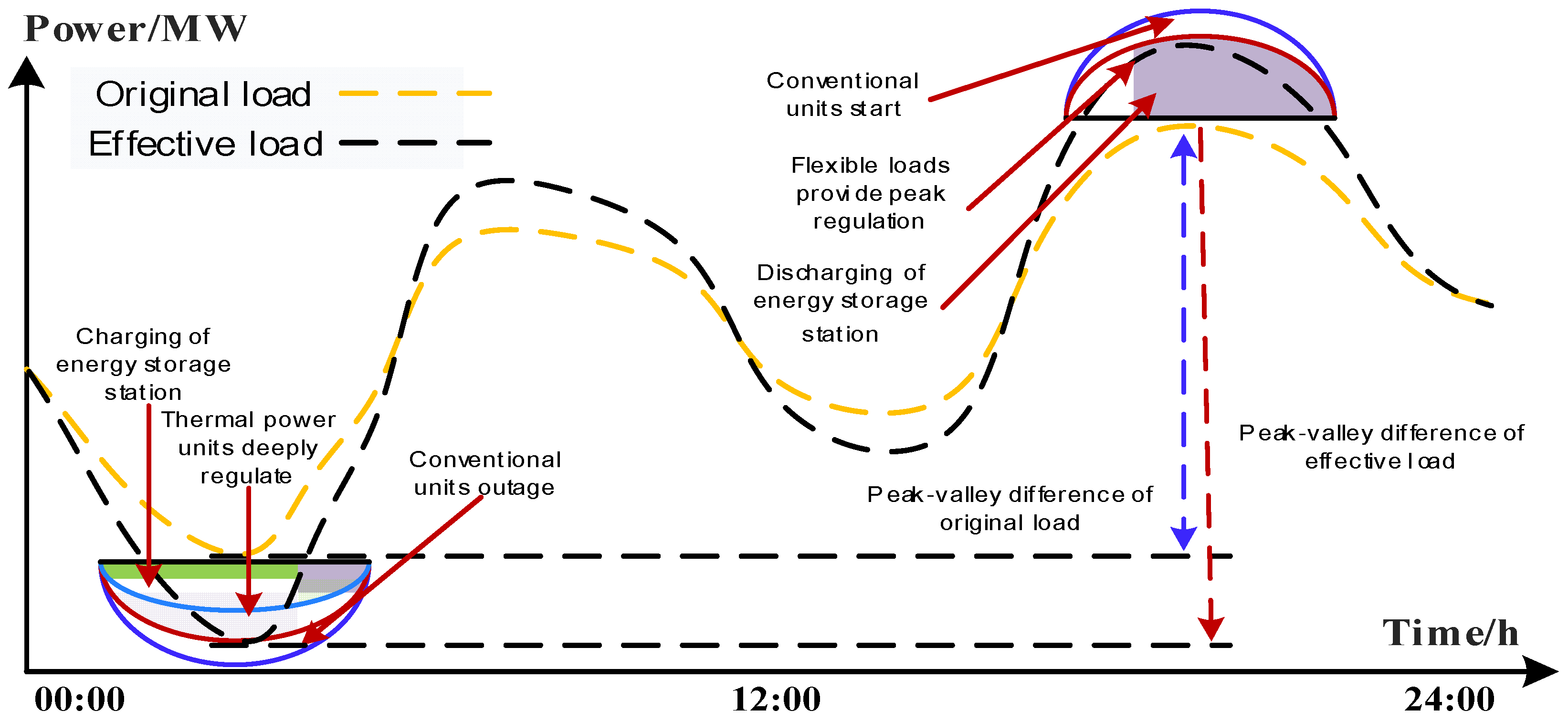
Based on current grid dispatching rules, during off-peak periods, when new energy is integrated and absorbed, if the output of conventional generators within the system exceeds their minimum technical output, the grid-integrated new energy does not incur peak regulation ancillary service costs. However, when the output of these conventional generators falls below their minimum technical output, the new energy integration bears the cost of peak regulation ancillary services. As the power from new energy integration increases, not only does the incurred peak regulation ancillary service cost rise, but the entities providing these services also vary [25], as shown in Figure 1. For instance, when the demand for peak regulation is low, the peak regulation ancillary service cost for the kth is:
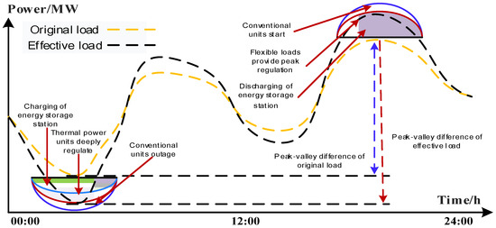
Figure 1.
Peak regulation ancillary serve caused by new energy generation grid connection.
Equation (1) depicts the cost calculation method when only energy storage stations participate, with and representing the price and maximum charging power of energy storage stations, respectively, during off-peak periods. When the demand for peak regulation further escalates, the cost is:
Equation (2) represents the cost calculation method when only energy storage stations charge and thermal power units deeply regulate, with and representing the price and maximum power of deep peak regulation by thermal power units, respectively, during off-peak periods. If the peak regulation demand increases even further, the cost is:
Equation (3) represents the cost calculation method when energy storage stations charge, thermal power units deeply regulate, and conventional units are shut down to provide peak regulation ancillary services. and symbolize the price and maximum power, respectively, when conventional units are shut down to offer these services.
In the above Equations (1)–(3), the method used to calculate the new energy integrated power that incurs peak regulation ancillary service costs is:
In this Equation, the first part represents the power of new energy grid integration that must bear peak regulation ancillary service costs during the period of the off-peak time when the output of the conventional generators is higher than their minimum technical output , which corresponds to a power of 0 in this situation. The second part denotes the power during the period when the output of conventional generators is below their minimum technical output. The power of new energy power generation connected to the grid needs to bear the peak-shaving auxiliary service fee, and the corresponding power at this time is , namely, the sum of the new energy generation power and the minimum technical output of the conventional units, minus the load power.
2.1.2. Peak Regulation Ancillary Service Cost Model during Peak Load Periods
In alignment with the mechanisms providing peak regulation ancillary services during off-peak periods, during peak load times when the load power () is less than the maximum output of the conventional generators within the system (), the power from new energy grid integration bearing peak regulation ancillary service costs is zero. However, when the load power surpasses the maximum output of conventional generators, the system needs to employ energy storage station discharging, flexible load power reduction, and the activation of some conventional units to ensure stable system operation, as shown in Figure 2. At this juncture, the power from new energy grid integration that incurs peak regulation ancillary service costs () is:
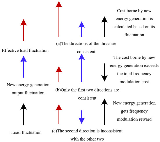
Figure 2.
Mechanism of frequency modulation costs undertaken by new energy generation output.
In this Equation, h denotes the sequence number of the peak load period, i.e., the hth period, with and representing the load power and new energy grid integration power, respectively, during the hth period.
During peak load periods, when the system’s demand for peak regulation ancillary services is minimal, the cost borne by new energy grid integration for these services is:
In this Equation, and are the price and maximum discharging power, respectively, of energy storage providing peak regulation ancillary services during peak periods. As the demand for such services further escalates, the cost borne by new energy grid integration is:
In this Equation, and represent the price and maximum power reduction possible, respectively, when flexible loads provide peak regulation ancillary services. If the system’s demand for these services grows even more, the cost borne by new energy grid integration is:
In this Equation, and signify the price and maximum power, respectively, when conventional units are activated to provide peak regulation ancillary services during peak periods.
2.2. Frequency Regulation Ancillary Service Costs Induced by New Energy Integration
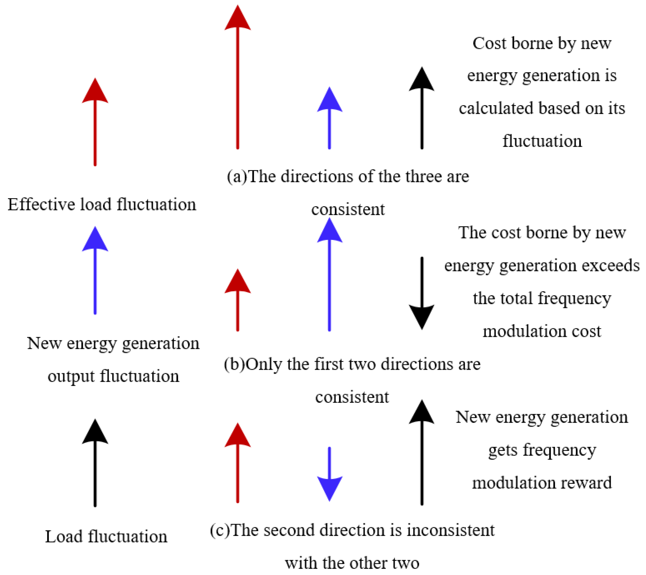
The frequency regulation ancillary services resulting from new energy grid integration are primarily determined by its influence on the effective grid load fluctuations (the difference between the original grid load and the power from new energy integration) [26]. Therefore, by analyzing the correlation between the directions of effective grid load fluctuations, original grid load power fluctuations, and new energy grid integration power fluctuations, a model to calculate the frequency regulation ancillary service costs induced by new energy grid integration is established. Figure 2 presents the mechanism of frequency modulation costs undertaken by the new energy generation output.
When the fluctuation directions of all three aforementioned factors align, the power fluctuations from new energy grid integration amplify the effective grid load power fluctuations. In such cases, the fluctuations from both the new energy grid integration and the original grid load should evenly share the costs induced by the effective grid load power fluctuations. The corresponding model to calculate the frequency regulation ancillary service costs () due to new energy grid integration power fluctuations is:
In this formula, represents the sequence number of the calculation period , i.e., the period. denotes the frequency regulation ancillary service costs induced by effective grid load power fluctuations, which is provided by the power dispatching center based on frequency regulation rules. and represent the fluctuations in the original grid load power and the power from new energy grid integration, respectively.
When the fluctuation direction of the original grid load power differs from the fluctuations of new energy grid integration power and effective grid load power, the original grid load power fluctuations effectively reduce the magnitude of the effective grid load power fluctuations. The corresponding model to calculate the frequency regulation ancillary service costs () due to new energy grid integration power fluctuations is:
In this Equation, fluctuations in the grid-integrated renewable power not only assume the grid’s frequency regulation ancillary service costs but also the contribution rewarded by the grid for the original load’s advantageous participation in frequency regulation services. For instance, certain flexible loads with superior modulation capabilities can actively partake in the grid’s frequency regulation services.
When the fluctuation direction of the renewable grid-integrated power is incongruent with both the grid’s effective load power and the original load power, the renewable power’s fluctuation effectively attenuates the grid’s effective load power fluctuation amplitude. This means that the original load power’s fluctuations not only bear the grid’s frequency regulation ancillary service costs but also the additional rewards for the renewable grid-integrated power’s beneficial contribution to these services. This strategy indirectly incentivizes renewable power plants to partake in the grid’s frequency regulation services. The calculation model for the frequency regulation auxiliary service fee () caused by the power fluctuation of the corresponding new energy power generation connected to the grid is expressed as:
2.3. Spinning Reserve Ancillary Service Costs Induced by New Energy Integration
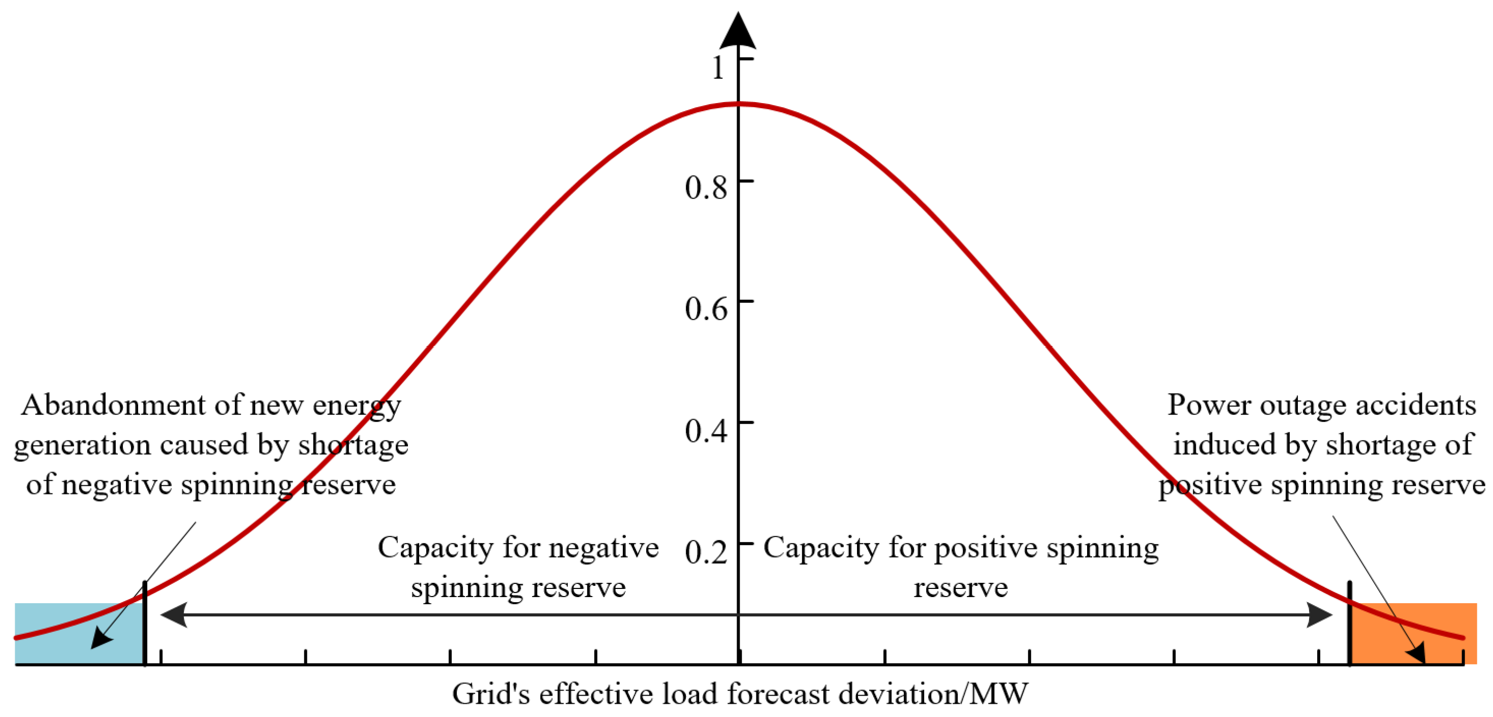
The spinning reserve ancillary services necessitated by new energy grid integration are predominantly governed by discrepancies in the grid’s effective load forecast. These deviations are jointly determined by the forecast variances in both the new energy grid-integrated power and the original grid load [27]. Assuming the probability distribution model for the grid’s effective load forecast deviation is (as both the original grid load forecast deviation and the renewable grid integration power forecast deviation are normally distributed), the costs that the grid incurs for spinning reserve ancillary services can be expressed as:
In this Equation, the price for spinning reserve ancillary services is denoted by , while and represent the system’s permissible maximum new energy curtailment rate and maximum load shedding rate, respectively. signifies the standard deviation of the grid’s effective load forecast deviation probability distribution. Stemming from this, the model to compute the spinning reserve ancillary service costs induced by new energy grid integration is defined as:
In this Equation, indicates the spinning reserve ancillary service costs as a result of the original grid load in the absence of new energy integration, defined as:
In this Equation, the original load forecast deviation probability distribution model is denoted by , which can be derived with appropriate modifications.
Figure 3 shows the impact of spinning reserve configuration on load shedding and new energy generation power discarding.
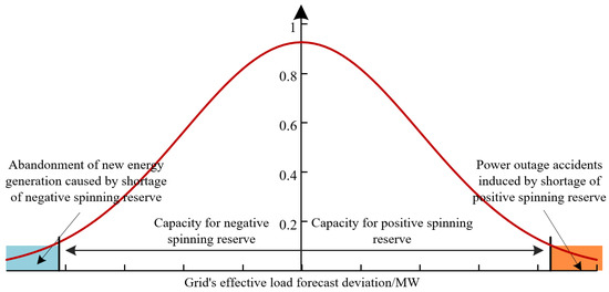
Figure 3.
Impact of spinning reserve configuration on load shedding and new energy generation power discarding.
3. Regional Grid Upper-Level Optimization Dispatch Model
Although the output of new energy power plants in wide areas has strong complementary characteristics, the complementary laws have strong time-varying characteristics. The output of new energy power plants is aggregated in different time periods, so that the new energy power plants can participate in grid scheduling in a cluster manner. This reduces the peak shaving and frequency regulation auxiliary service costs caused by the grid connection of new energy power plants, as well as the difficulty of scheduling plan formulation and its implementation for new energy generation integration systems [27].
Due to the complexity of meteorological factors and the inaccuracy of prediction models, the degree to which new energy generation output can be accurately predicted gradually decreases with the increase of prediction timescale [5]. That is to say, in the process of grid optimization and scheduling, if only weekly or daily trading models are selected for auxiliary service market transactions, the large prediction deviation of new energy generation output may lead to significant auxiliary service costs for its integration into the system. Conversely, if auxiliary service market transactions are conducted at shorter intervals (such as intraday trading or trading within tens of minutes to several hours), a lot of auxiliary service costs will be saved due to the higher prediction accuracy of new energy generation output [28]. Taking wind power as an example, its output remains relatively constant within 10 min.
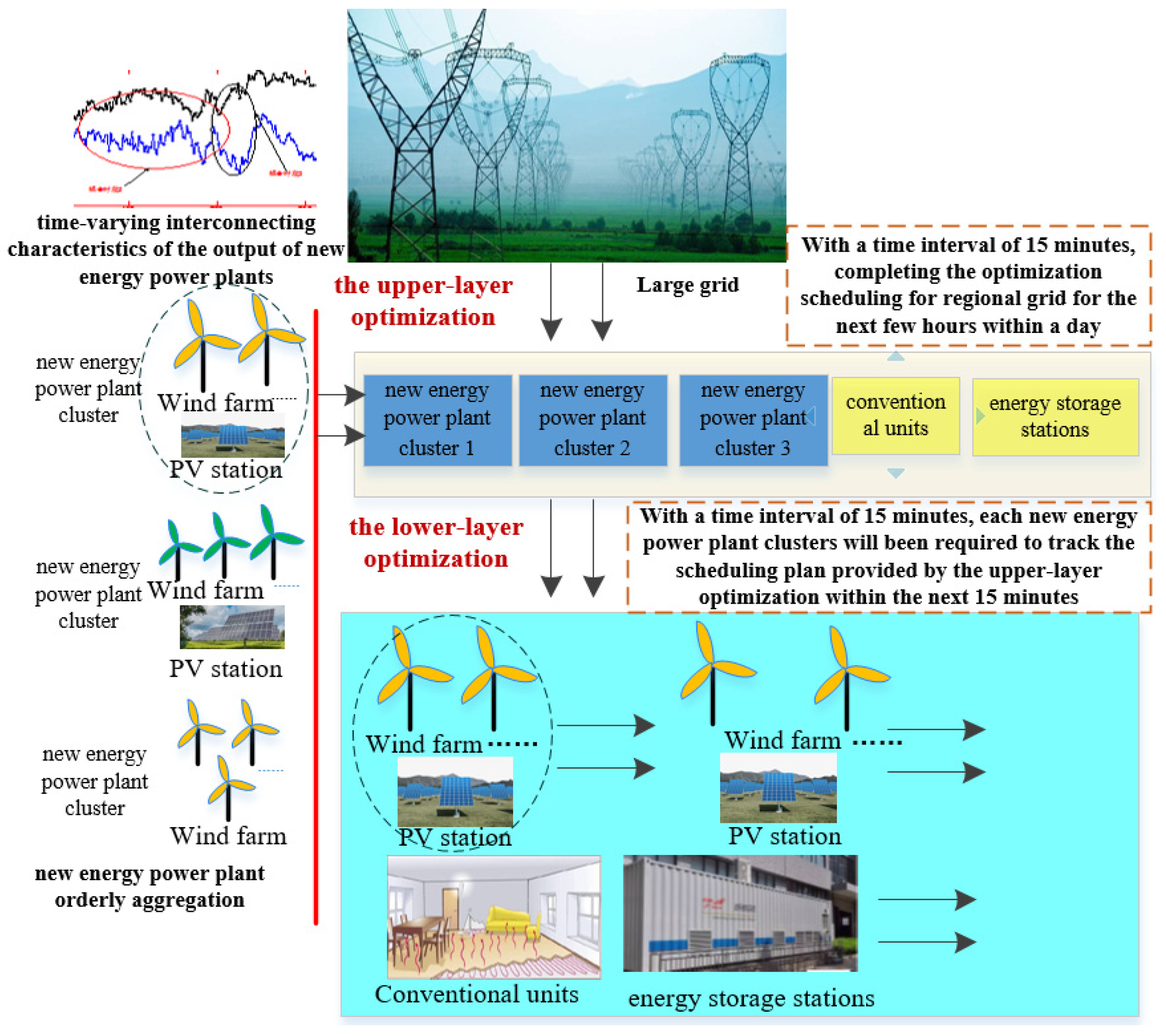
Referring to the overall grid dispatching architecture in China (which can been divided into five levels: national dispatch, grid dispatch, provincial dispatch, regional dispatch centers, and county-level dispatch centers) as well as the existing coordination and control methods for virtual power plants/groups participating in grid dispatch [2,6,29,30,31,32], a basic architecture for dual level optimization dispatch for regional grids with new energy power plant clusters is proposed in this paper, as shown in Figure 4. In the dispatching architecture, the upper-layer optimization completes the optimization scheduling for regional grid for the next few hours within the day (with a time interval of 15 min), including the planned output of new energy power plants/clusters obtained by the orderly aggregation, conventional units, energy storage stations, and flexible loads. In the lower optimization, each new energy power plant cluster will be required to track the scheduling plan provided by the upper-layer optimization within the next 15 min (with a time interval of 5 min).
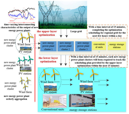
Figure 4.
The basic bi-level optimization dispatch architecture for regional grids.
Building upon the ancillary service cost computation models for grid-integrated new energy, established in Section 2, this section formulates the upper-level optimization dispatch model for the regional grid. This model takes into account the ancillary service costs associated with new energy grid integration and aims to optimize grid operations for the forthcoming hours.
3.1. Objective Function in the Upper-Level Optimization Dispatch Model
In light of the findings in Section 1, the types of ancillary services required due to grid-integrated new energy might differ across load periods. Hence, this study delineates the upper-level optimization dispatch models for three distinct load periods: off-peak, normal, and peak.
3.1.1. Objective Function for the Off-Peak Load Period
During off-peak periods, the primary ancillary services induced by new energy grid integration encompass load leveling, frequency regulation, and spinning reserve services. To optimize the overall operational benefits of the regional grid, the overarching objective is to minimize the sum () of the grid’s energy procurement costs and ancillary service acquisition costs. The corresponding objective function for the off-peak period in the upper-level optimization dispatch model is given by:
In this Equation, i denotes the index for computation cycles during off-peak periods, with a total of cycles. The first three terms in the equation represent the cumulative energy procurement costs from the grid, specifically from conventional power generating units, energy storage stations, and clusters of new energy plants. and , and , and and denote the prices and power of these three entities during energy transactions, respectively. The subsequent three terms represent the costs of load leveling, frequency regulation, and spinning reserve services induced by grid-integrated new energy, corresponding to Equations (1), (9), and (13) from Section 1.
In Equation (8), indicates the pricing for grid integration of new energy clusters. Given that these clusters might comprise both photovoltaic stations and wind farms, the pricing for energy transactions provided by each new energy plant within the cluster is deduced as:
In this Equation, represents the collection of the lth new energy cluster and and indicate the grid integration price and power, respectively, for the new energy plant during the ith cycle in .
3.1.2. Objective Function for the Normal Load Period in Upper-Level
Optimization Dispatch
During the normal load period, the ancillary services induced by grid-integrated new energy encompass frequency regulation services and spinning reserve services. Thus, the objective function for this period in the upper-level optimization dispatch model for the regional grid is described by:
In this Equation, the first three terms have meanings analogous to those in Equation (15) and are thus not reiterated here. The subsequent two terms represent the costs of frequency regulation services and spinning reserve services induced by grid-integrated new energy, specifically referring to Equations (9) and (13).
3.1.3. Upper-Level Optimization Dispatch Model for Peak Load Period
During peak load periods, due to the counter-peaking characteristics of grid-integrated new energy power (manifested as a decline in grid-integrated new energy power as the load increases) or the low reliability of new energy plant capacity [24,25], there may arise scenarios in which the frequency is too low, or even load shedding accidents. Consequently, the ancillary services induced during peak load periods include load leveling, frequency regulation, and spinning reserve services. The corresponding objective function in the upper-level optimization dispatch model is:
In this Equation, both the first three terms and the subsequent three terms have meanings similar to those in Equation (15) and are thus not reiterated. Specifically, the fourth term in this equation represents the load leveling service costs induced by grid-integrated new energy during the ith cycle of the peak load period, referring to Equations (6)–(8).
3.2. Constraints in the Upper-Level Optimization Dispatch Model
To ensure the stable operation of the system, the grid-integrated new energy system must satisfy power balance constraints. Conventional power generation units should operate within permissible power ranges; energy storage stations should operate within allowable power and SOC (state of charge) ranges; the power reduction of flexible loads should be less than their allowable power reduction; and the planned grid integration power of new energy clusters should be less than their forecasted power. Due to space constraints in this paper and since these concepts are easily comprehensible, they are not elaborated upon here.
In the system’s spinning reserve optimal allocation, the allocated spinning reserve should not only suppress the predictive bias of the grid’s equivalent load but also restrain its fluctuations. This means the allocated spinning reserve should consider both adjustment capacity and adjustment rate requirements, as follows:
The above equation implies that the capacity of the allocated spinning reserve should meet the grid’s equivalent load prediction bias requirements. Here, and represent the positive spinning reserve capacity and the negative spinning reserve capacity allocated for the regional grid in the cycle, respectively, preventing load shedding accidents and the curtailment of new energy generation. and respectively denote the predictive biases of grid-integrated new energy power and the original grid load in the aforementioned calculation cycle, being the sum of both predictive biases.
Furthermore, the adjustment rate considered during spinning reserve allocation targets the fluctuations of the grid’s equivalent load [24,25], as described by:
In this equation, and respectively represent the maximum values of the allocated spinning reserve for the regional grid during the cycle. and denote the fluctuation quantities of grid-integrated new energy power and the original grid load during the above calculation cycle, respectively. is the sum of both fluctuation quantities.
4. Lower-Level Optimization Dispatch Model for the Regional Grid
Similar to the structure presented in Section 2, the lower-level optimization dispatch model for the regional grid also comprises two main components: the objective function and associated constraints.
4.1. Objective Function in the Lower-Level Optimization Dispatch Model
Building on the content from Section 2, the significance of constructing the upper-level optimization dispatch model for the regional grid lies in providing results for several hours of optimized dispatch. This aims to reduce the grid’s energy procurement costs and ancillary service costs. However, the randomness in new energy generation and load power fluctuations can make it challenging to execute the upper-level optimization dispatch results with absolute accuracy. Nevertheless, from the perspective of the grid’s overall economic performance, the results from the upper-level optimization dispatch undoubtedly represent an optimal value. Therefore, the importance of constructing the lower-level optimization dispatch model emphasizes the accurate tracking by each new energy plant cluster of the demands set by the upper-level optimization dispatch. The corresponding objective function in the lower-level optimization dispatch model is described by:
In this Equation, represents the total number of cycles in the lower-level optimization process (each cycle being 5 min); denotes the total number of new energy plant clusters; and and are the actual output and the planned output during the lower-level optimization process, respectively, with illustrating their difference. Given that the time interval in the upper-level optimization process is 15 min and that in the lower-level optimization process is 5 min, this paper employs a two-point linear interpolation method to fill the output plan of the new energy plant cluster between two adjacent moments within the 15 min time range of the upper-level optimization process, which is not detailed further here.
During the lower-level optimization dispatch process for the regional grid, the actual output of a new energy plant cluster might exceed the dispatch plan provided by the upper-level optimization dispatch model. Consequently, new energy plants within the cluster could face wind curtailment or solar curtailment issues. Although, from the perspective of prioritizing new energy consumption, all new energy outputs should be wholly consumed, considering the overall economic requirements of grid operation, the grid permits curtailment during certain periods or for specific new energy plants [27]. Accordingly, taking into account the equal requirements for wind/solar curtailment losses, the wind/solar curtailment model for each new energy plant during the curtailment process of the new energy plant cluster is constructed as:
In this Equation, represents the cumulative absolute value of the difference in wind/solar curtailment losses for each new energy plant within the ith new energy plant cluster during the rth cycle of the lower-level optimization dispatch process. Here, signifies the wind/solar curtailment loss of the ith new energy plant within the Ith cluster during that period. The term denotes that the actual output of the new energy plant cluster exceeds the planned output provided by the upper-level optimization dispatch model, indicating that the cluster faces wind/solar curtailment issues.
4.2. Constraints in the Lower-Level Optimization Dispatch Model
Following the same logic used in constructing constraints for the upper-level optimization dispatch process, the lower-level optimization dispatch should also consider power balance constraints, stable operating constraints for conventional generators, energy storage stations, and flexible loads. The configured spinning reserves should meet both the grid equivalent load forecast deviation and fluctuation constraints. Moreover, considering the varying forecast accuracy of new energy generation outputs at different timescales, and that the upper and lower-level optimizations are executed over several hours and several tens of minutes, respectively, we specifically outline the output constraints for the new energy plant cluster and its internal new energy plants during the lower-level optimization dispatch process as:
The above equation represent the planned output and the forecasted maximum output of the ith new energy plant cluster during the ith cycle of the lower-level optimization process, respectively. The corresponding calculation method is described in:
In this Equation, and denote the planned output and the forecasted maximum output, respectively, for the jth new energy plant during the ith cycle.
5. Solution of the Two-Layer Optimal Dispatching Model for Regional Power Grid
Based on the above content and discussion, the bi-lever optimized dispatching method for high penetration new energy power grids proposed in this paper is designed to solve optimized dispatching problem in several hours. In this double-layer dispatching framework, the upper-layer optimization completes grid optimization for several hours, which presents the planned output of conventional units, energy storage stations, and new energy power plants/clusters, with the objective of minimizing both grid energy procurement costs and ancillary service trading costs. The purpose of the lower-layer optimization is to make new energy plants/clusters follow the upper-layer optimization plans as closely as possible, accomplishing grid optimization for several tens of minutes, while ensuring equalized wind and solar curtailment losses within new energy plant cluster. Hence, both the upper-layer and lower-layer optimized dispatching models can be characterized as single objective and multi-variable problems. The two optimized dispatching models will be solved by variable step particle swarm optimization (VSPSO), as shown in Figure 5.
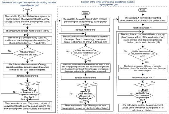
Figure 5.
Solving process of the two-layer optimal dispatching model for regional power grids.
- (1)
- Solution of the upper layer optimal dispatching model of regional power grids
Step 1: the variable Xor,rn = [xG,1, …… xG,n, xS,1, …… xS,m, xre,1, …… xre,k] is initialized firstly, which presents the planned outputs of conventional units, energy storage stations, and new energy power plants/clusters. The subscript variables n, m, and k indicate the number of the above systems, respectively.
Step 2: the initial population Xor,rn is brought into the objectives of the upper-layer optimized dispatching models (as shown in Equations (15), (17), and (18)). Then, the sum of grid energy trading costs and ancillary service trading costs is calculated. Simultaneously, these constraints must be met in Section 3.2 of this paper, such as energy supply and demand balance in regional power grid, spinning reserve compensating forecast deviation, and fluctuation of grid equivalent load reliably, and the safe and stable operation request of each system participating in energy market transactions and ancillary service market transactions.
Step 3: the velocity and position of the population Xor,rn is uploaded and the uploaded population Xgx,rn is obtained.
Step 4: the above uploaded population Xgx,rn is brought into step 2 and then the sum of grid energy trading costs and ancillary service trading costs is regained, while meeting the constrains in Section 3.2 of this paper.
Step 5: these operations of step 2 to 4 are repeated until the minimum sum of grid energy trading costs and ancillary service trading costs is achieved. At the same time, the constrains in Section 3.2 of this paper are met. These calculated results present the planned outputs of conventional units, energy storage stations, and new energy power plants/clusters in several hours.
- (2)
- Solution of the lower-layer optimized dispatching model
Step 1: the variable Xor,realt = [xre,1, …… xG,ƞ] is initiated firstly, which presents the planned outputs of new energy power plants/clusters in several minutes. The subscript variable ƞ presents the number of new energy power plants/clusters.
Step 2: the initialed population Xor,realt is brought into the objective of the lower-layer optimized dispatching model (as shown in Equation (21) in Section 4.1 of this paper). The absolute accumulated difference between the output of each new energy power plant cluster from the lower-layer optimized dispatching model and the output from the upper-layer optimized dispatching models is obtained, while meeting the constrains in Section 4.2 (such as Equations (23) and (24) of this paper).
Step 3: the velocity and position of the population Xor,realt is uploaded and the uploaded population Xgx,realt is obtained.
Step 4: the uploaded population Xgx,realt is brought into Step 2. The absolute accumulated difference is obtained again and these constrains must also be met at the same time, which is similar to the content in step 2.
Step 5: the operations of step 2 to 4 are repeated until the minimum absolute accumulated difference is achieved, meeting the constrains simultaneously, as in step 2 or step 4. Every new energy plant cluster output in several minutes is gained.
Some aspects of the solution progress of the bi-lever optimized dispatching model must be emphasized: (1) the number of the swarm population is 40. Both the learning factor C1 and C2 are set to 2; (2) the inertia coefficient W is set 1; and (3) the maximum iteration number is set to 500 or the iteration is finished when the result of four consecutive iterations is less than 0.0001.
- (3)
- Solution of abandonment model of wind/solar power plants within the new energy power plant group by Genetic Algorithm (GA)
Step 1: the variable X = [x1, ……, xπ] is initialed, which presents the abandonment value of wind/solar power plants within the new energy power plant group. The subscript variable π presents the number of new energy plants in the new energy power plant group with the abandonment existence of wind/solar power plants.
Step 2: the absolute accumulated difference among abandonment values of the wind/solar power plants in real-time dispatching stage is obtained (as shown in Equation (22)), meeting the constrains in Section 4.2 of this paper (as shown in Equations (23) and (24)).
Step 3: the uploaded population Xby is obtained by cross and variation method.
Step 4: the uploaded population Xby is brought into step 2 instead of X. The absolute accumulated difference is calculated again.
Step 5: the operations of step 2 to 4 are repeated until the minimum absolute accumulated difference is obtained.
6. Simulation Study
6.1. Introduction to the Simulation
This paper employs operational data from a new high-penetration regional energy grid in Northern Xinjiang on 16 November 2018 to validate the feasibility of the proposed bi-level optimization dispatch method for grids with significant renewable penetration, factoring in ancillary service costs. The simulation includes: (1) thirteen new energy plants: plants numbered 7–9 are photovoltaic stations with a capacity of 20 MW, those numbered 1–6 are wind farms with a capacity of 49.5 MW, and those numbered 10–13 are wind farms with a capacity of 100 MW; (2) four conventional generators: units 1–2 operate using a “combined heat and power” mode, while unit 3 can operate in a deep peaking mode, with a peaking price set at 20.87 USD/(MW·h) [25]; (3) two pumped storage stations with a capacity of 240 WM·h, with maximum charging and discharging capacities set at 60 MW and 40 MW, respectively. The peak shaving ancillary service price is 16.00 USD/(MW·h) [33]; (4) during peak load periods, the flexible load capacity available for peak shaving ancillary services is 8.3 MW, with a service price of 20.83 USD/(MW·h) [34]; (5) frequency regulation ancillary services are entirely provided by conventional generators, with a frequency regulation price set at 0.83 USD/MW [35]; (6) the grid equivalent load standard deviation stands at 7.19 MW. When both and are set at 0.5%, the required spinning reserve capacity increases by 9.09 MW. Given a reserve cost of 0.003 USD/kW·h, an additional 13.91 USD per cycle is needed for the spinning reserve ancillary service cost [36].
6.2. Simulation Results and Analysis
Adopting the prevailing grid operational time-slot allocation, the periods from 00:00 to 08:00 are designated as off-peak hours, 08:00 to 14:30 as morning peak hours, 14:30 to 19:30 as standard operational hours, and 19:30 to 24:00 as evening peak hours. Given the constraints of paper length and the need for concise presentation, only the grid operational results during the off-peak and morning peak periods are analyzed. In the following discussion, Scheme 1 refers to the bi-level optimization dispatch method for grids with high renewable penetration proposed in this paper, which takes into account the costs of grid-connected ancillary services. In contrast, Scheme 2 denotes the optimization dispatch method without considering the costs of grid-connected ancillary services.
6.2.1. Off-Peak Period
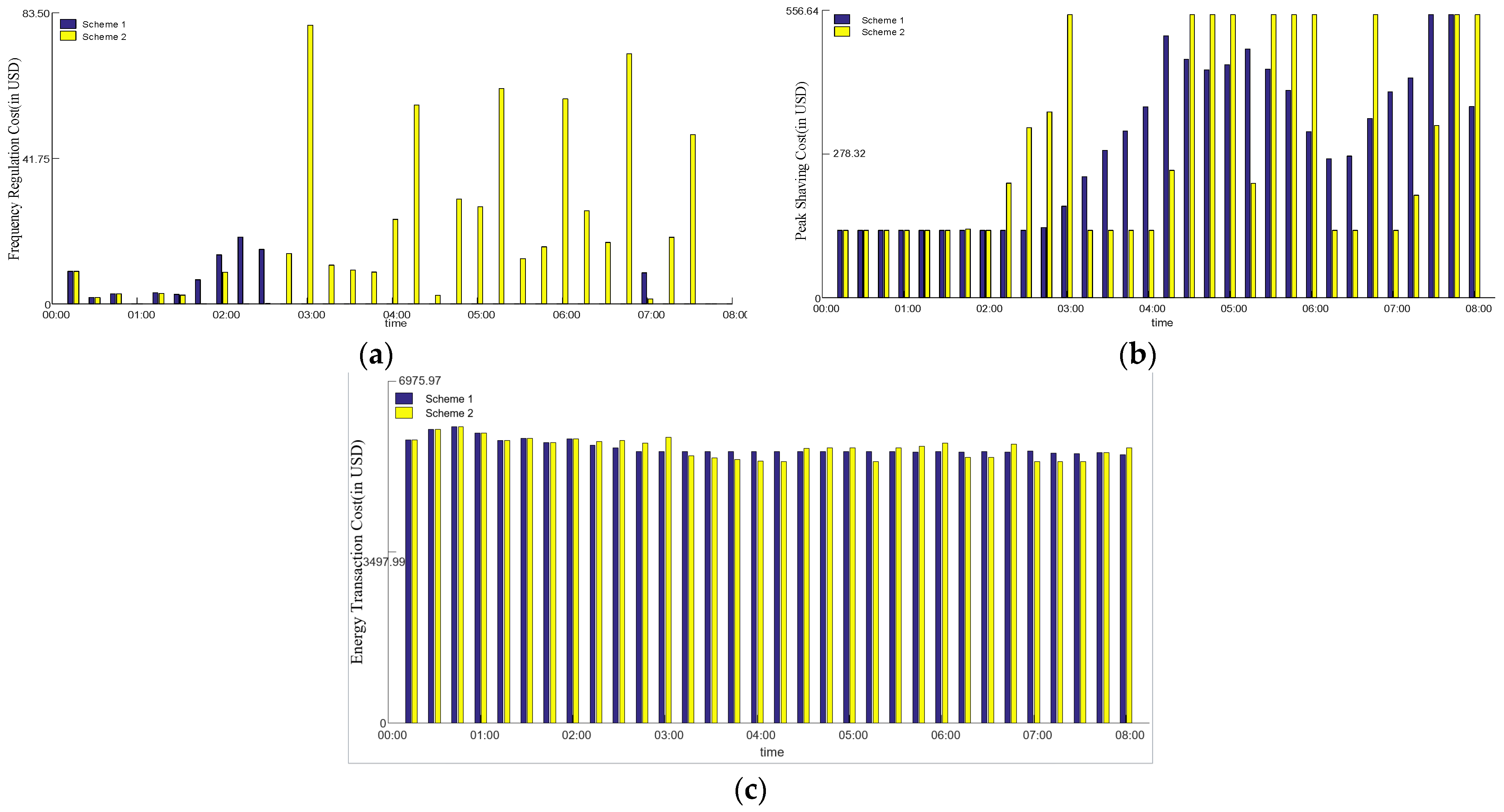
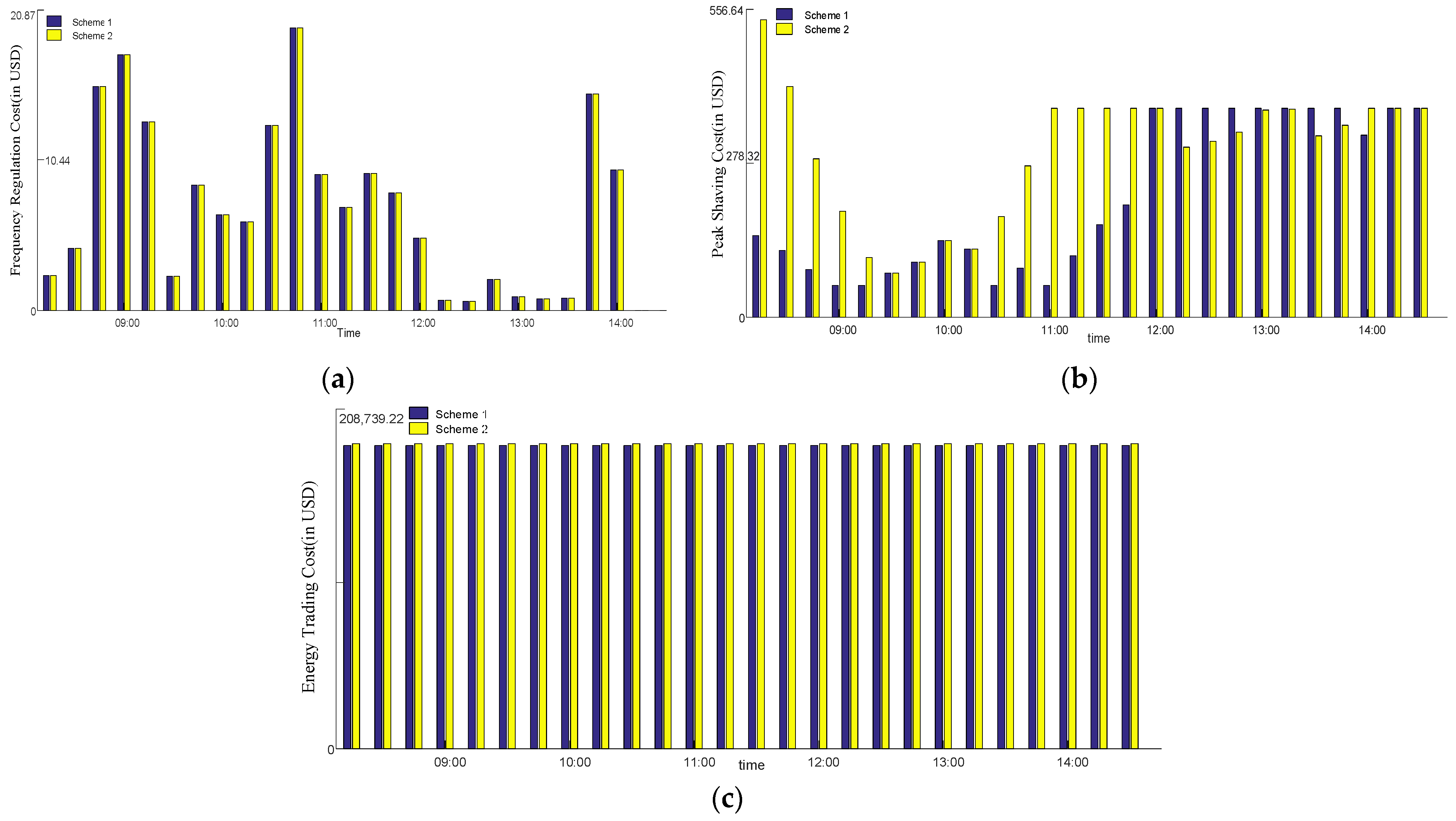
Figure 6 presents the costs incurred for ancillary services and energy transactions during the off-peak period. The analysis reveals: (1) regarding the frequency regulation ancillary service costs, the expenses induced by the grid-connected new energy generation under Scheme 1 and Scheme 2 are 8.49 USD and 63.08 USD, respectively. This indicates that Scheme 1 significantly reduces the frequency regulation ancillary service costs induced by grid-connected new energy generation; (2) pertaining to the peak shaving ancillary service costs, the expenses induced by the grid-connected new energy generation under Scheme 1 and Scheme 2 are 914.82 USD and 935.00 USD, respectively. This implies that Scheme 1 saves on peak shaving ancillary service costs compared to Scheme 2; (3) for the off-peak period, the energy transaction costs under Scheme 1 and Scheme 2 are 17,826.33 USD and 17,937.66 USD, respectively, signifying that Scheme 1 results in savings in energy transaction costs compared to Scheme 2.

Figure 6.
The upper dispatching model simulation results during load valley period: (a) frequency regulation ancillary service cost; (b) peak shaving ancillary service cost; (c) energy transaction expenditure.
Furthermore, considering that spinning reserves mainly address grid equivalent load forecasting deviations and fluctuations [26], both schemes require an additional positive and negative spinning reserve of 9.09 MW. Thus, the auxiliary service cost induced by grid-connected new energy generation for spinning reserves remains constant for every cycle, which is not presented here.
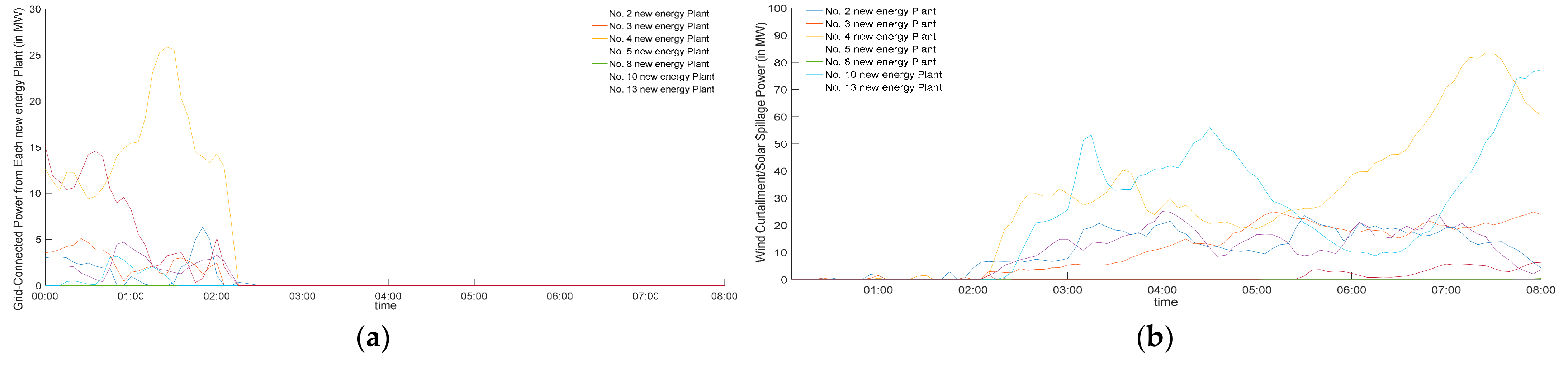
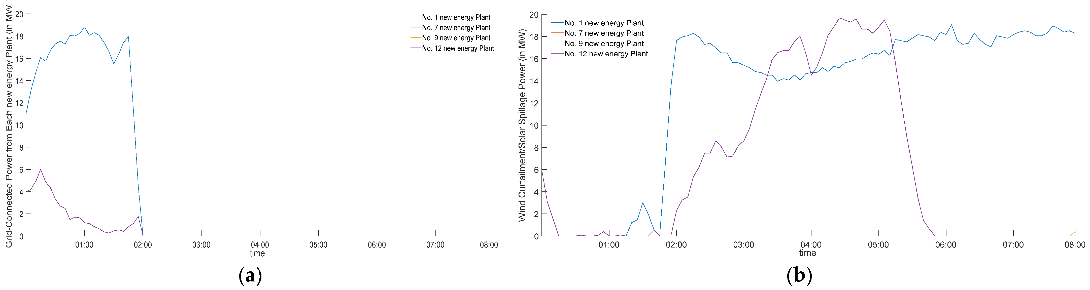
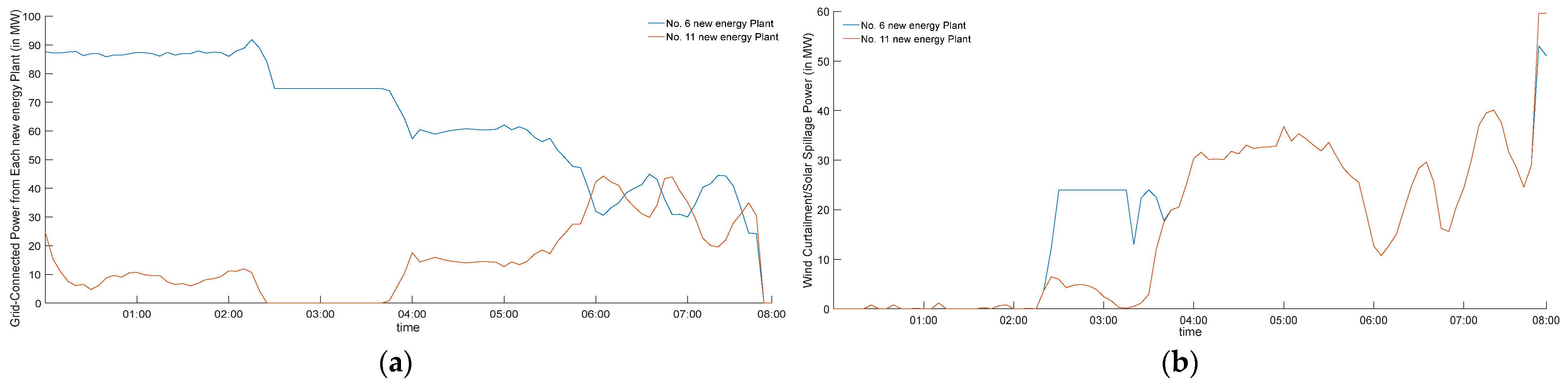
Figure 7, Figure 8 and Figure 9 respectively present the optimized dispatching results of the new energy power plant groups during the load valley period when applying the lower-level optimization dispatching scheme proposed in this paper. Analysis indicates the following: (1) during the lower-level optimization dispatching process of the regional power grid, the 1st and 2nd new energy power plant groups can be fully integrated into the grid during the initial period (approximately 00:00 to 02:00). However, as time progresses, the grid’s original load further decreases and the reservoir capacity of the pumped storage power station reduces, leading to the withdrawal of the 1st and 2nd new energy power plant groups from grid dispatching, resulting in curtailment of new energy generation; (2) compared to the 1st and 2nd new energy power plant groups, although the 3rd new energy power plant group also experiences some wind curtailment after 02:00 due to system absorption constraints, its relatively lower grid clearing price ensures its continuous participation in grid dispatching; (3) during the curtailment of new energy generation by the new energy power plant groups, the losses from curtailed new energy generation are evenly distributed within the group as much as possible. For instance, after 02:00, when the 3rd new energy power plant group faces curtailment, the wind curtailment losses are evenly shared between the two wind farms. This observation corroborates the fairness and rationality of the wind/solar curtailment scheme in the lower-level optimization dispatching model established in this paper.
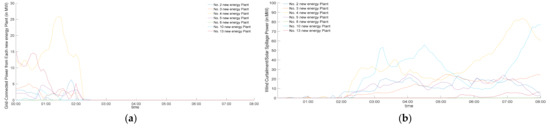
Figure 7.
The dispatching results of No. 1 new energy power plant group during lower level optimization dispatching of the power grid: (a) actual grid-connected power from each new energy plant; (b) wind curtailment/solar spillage power from each new energy plant.
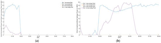
Figure 8.
The dispatching results of No. 2 new energy power plant group during lower level optimization dispatching of the power grid: (a) actual grid-connected power from each new energy plant; (b) wind curtailment/solar spillage power from each new energy plant.
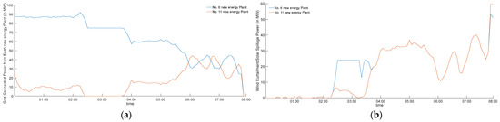
Figure 9.
The dispatching results of No. 3 new energy power plant group during lower level optimization dispatching of the power grid: (a) actual grid-connected power from each new energy plant; (b) wind curtailment/solar spillage power from each new energy plant.
6.2.2. Load Peak Period in the Early Morning
Figure 10 displays the results of the upper-level optimization dispatching during the early morning load peak period. Analysis reveals that: (1) during the early morning load peak period, with the increase of the original grid load, the output of the 1st and 2nd new energy power plant groups can be fully integrated into the grid. Under both Scheme 1 and Scheme 2, the ancillary service costs for frequency regulation induced by the integration of new energy generation remain consistentl; (2) during the early morning load peak period, under most time intervals, Scheme 1 incurs lower ancillary service costs for load leveling induced by new energy integration compared to Scheme 2. This demonstrates that the bi-level optimization dispatching method established in this paper, which considers ancillary service costs, can significantly reduce the load leveling ancillary service expenses caused by the integration of new energy; (3) the energy trading costs under Scheme 1 and Scheme 2 are 4,834,167.27 USD and 4,874,060.67 USD, respectively, suggesting that the bi-level optimization dispatching method proposed in this paper, which takes into account ancillary service costs, can also reduce energy trading costs.

Figure 10.
The upper dispatching model simulation results during first load peak period: (a) frequency regulation ancillary service cost; (b) peak shaving ancillary service cost; (c) energy trading cost.
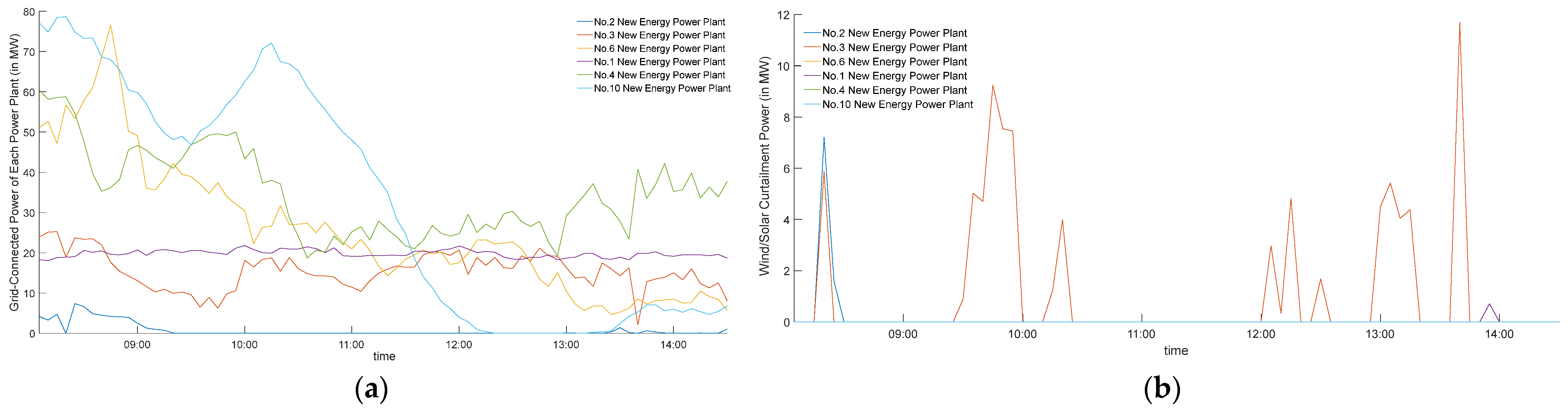
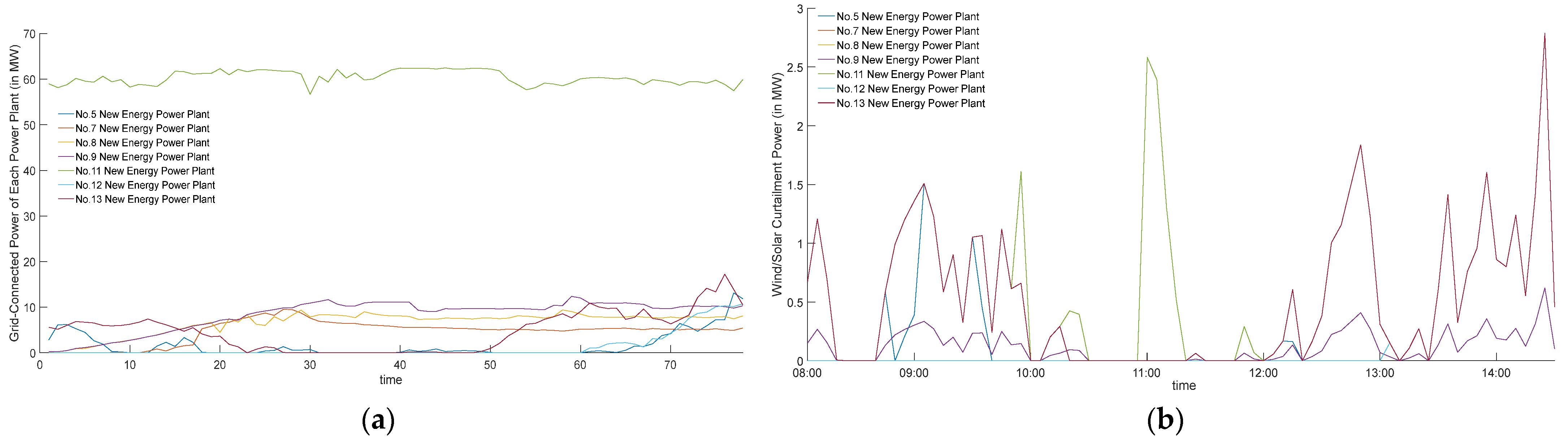
Figure 11 and Figure 12 respectively present the optimized dispatching results of new energy power plant groups during the early morning load peak period using the lower-level optimization dispatching of the regional grid. From the analysis, it can be inferred that: (1) due to the bi-level optimization dispatching model established in this paper, which respectively realizes several hours of grid optimization dispatching and several tens of minutes of optimization dispatching, the upper-level optimization dispatching model and the lower-level optimization dispatching model are based on different timescale predictions of new energy power output. Therefore, during the early morning load peak period, when the lower-level optimization dispatching model is implemented, there are occasional instances of a small amount of new energy being discarded in the 1st and 2nd new energy power plant groups; (2) when the 1st and 2nd new energy power plant groups have a slight amount of discarded new energy, the loss of wind curtailment/solar curtailment is as evenly distributed as possible among the new energy power plants within the group, further corroborating the fairness and rationality of the wind/solar curtailment scheme in the grid lower-level optimization dispatching model established in this paper.
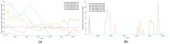
Figure 11.
The grid connected power of each power plant in the No. 1 new energy power plant group during the first load peak period: (a) grid-connected power of each power plant; (b) wind/solar curtailment power of each power plant.
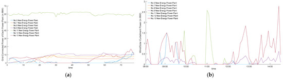
Figure 12.
The grid connected power of each power plant in the No. 2 new energy power plant group during first load peak period: (a) grid-connected power of each power plant; (b) wind/solar curtailment power of each power plant.
7. Conclusions
(1) To address the elevated ancillary service costs resulting from the grid integration of new energy power generation, this study introduces a bi-level optimization dispatching method for grids with high penetration of new energy, considering grid ancillary service costs. The upper-level optimization dispatching model carries out several-hour grid optimization, primarily aimed at saving ancillary service costs and grid energy procurement costs induced by the new energy grid connection. The lower-level optimization achieves optimization dispatching in tens of minutes, focusing on ensuring that new energy power plants/groups closely follow the upper-level dispatching plan.
(2) Compared with the traditional optimization dispatching methods for grids with high penetration of new energy, the proposed bi-level optimization dispatching method not only saves on the ancillary service costs caused by the new energy grid connection but also reduces grid energy procurement costs.
(3) During the implementation of the lower-level optimization dispatching, when the output of the new energy power plant/group might exceed the dispatching plan provided by the upper-level optimization dispatching model, the wind/solar curtailment model established in this paper ensures that the losses from wind/solar curtailment are evenly distributed among different new energy power plants within the group, guaranteeing balanced grid integration benefits for each new energy power plant.
(4) Since the bi-level optimization dispatching model for grids with high penetration of new energy, taking into account grid ancillary service costs, is based on new energy power output predictions on different timescales, there might be occasional instances where individual new energy power plant groups have a slight amount of discarded new energy during certain periods in the lower-level optimization dispatching process.
Author Contributions
Conceptualization, R.T. and F.L.; methodology, R.T.; software, Y.L.; validation, R.T., F.L., and Y.L.; formal analysis, Y.L.; investigation, F.L.; resources, R.T.; data curation, F.L.; writing—original draft preparation, R.T.; writing—review and editing, R.T.; visualization, F.L.; supervision, Y.L.; project administration, F.L.; funding acquisition, R.T. All authors have read and agreed to the published version of the manuscript.
Funding
This research was funded by the Chinese National Natural Science Foundation (No. 51767023) and Fuyang Normal University PhD Initiation Project (2020KYQD0001).
Data Availability Statement
The data presented in this study are available on request from the corresponding author. The reason the data and details in the simulation study part are not publicly available is that Xinjiang Power Grid in China does not allow the public disclosure of operational data for operational safety reasons.
Conflicts of Interest
The authors declare no conflicts of interest.
References
- Sha, Q.; Wang, W.; Wang, H. A Distributionally Robust Chance-Constrained Unit Commitment with N-1 Security and Renewable Generation. Energies 2021, 14, 5618. [Google Scholar] [CrossRef]
- Xin, Y.; Shi, J.; Zhou, J.; Gao, Z.; Yan, J. The Overall Architecture of Smart Grid Dispatching Control System, 1st ed.; China Electric Power Press: Beijing, China, 2016; pp. 174–298. [Google Scholar]
- Gong, G.; Wang, H.; Zhang, T.; Chen, Z.; Wei, P.; Su, C.; Wem, Y.; Liu, X. Research on electricity market about spot trading based on blockchain. Proc. CSEE 2018, 38, 6955–6966. [Google Scholar]
- North Star Electric News Network. Available online: https://news.bjx.com.cn/topics/xjdlfzfw/ (accessed on 10 September 2023).
- Safari, N.; Chung, C.Y.; Price, G.C.D. A Novel Multi-Step Short-Term Wind Power Prediction Framework Based on Chaotic Time Series Analysis and Singular Spectrum Analysis. IEEE Trans. Power Syst. 2017, 33, 590–601. [Google Scholar] [CrossRef]
- Guo, H.; Bai, H.; Liu, L.; Wang, Y. Optimal scheduling model of virtual power plant in a unified electricity trading market. Trans. China Electrotech. Soc. 2015, 30, 136–145. [Google Scholar]
- Meng, X.; Gao, J.; Sheng, W.; Gu, W.; Fan, W. A day-ahead two-stage optimal scheduling model for distribution network containing distributed generations. Power Syst. Technol. 2015, 39, 1294–1300. [Google Scholar]
- Li, B.; Li, X.; Bai, X.; Li, W. A Research on the IL Control Strategy of Distribution Network in Electricity Market. Proc. CSEE 2018, 38, 6573–6582. [Google Scholar]
- Sun, Y.; Wang, Y.; Wang, B. Multi-time scale decision method for source-load interaction considering demand response uncertainty. Autom. Electr. Power Syst. 2018, 42, 106–113. [Google Scholar]
- Qiu, H.; Zhao, B.; Gu, W.; Bo, R. Bi-level two-stage robust optimal scheduling for AC/DC hybrid multi-microgrids. IEEE Trans. Smart Grid 2018, 9, 5455–5466. [Google Scholar] [CrossRef]
- Tan, Z.F.; Ju, L.W.; Li, H.H.; Li, J.Y.; Zhang, H.J. A two-stage scheduling optimization model and solution algorithm for wind power and energy storage system considering uncertainty and demand response. Int. J. Electr. Power Energy Syst. 2014, 63, 1057–1069. [Google Scholar] [CrossRef]
- Liang, N.; Deng, C.; Tan, J.; Chen, Y.; Xia, P.; Liang, X. Optimization Scheduling with Multiple Time Scale for Active Distribution Network Considering Electricity Price Elasticity. Autom. Electr. Power Syst. 2018, 42, 44–50. [Google Scholar]
- Liu, Q.; Xie, P.; Ouyang, J.; Zhu, J.; Xiong, X.; Xuan, P. Dynamic economic dispatch strategy based on multi-time scale complementarity of heterogeneous energy sources. Electr. Power Autom. Equip. 2018, 38, 55–64. [Google Scholar]
- Hedayati-Mehdiabadi, M.; Zhang, J.; Hedman, K.W. Wind power dispatch margin for flexible energy and reserve scheduling with increased wind generation. IEEE Trans. Sustain. Energy 2015, 6, 1543–1552. [Google Scholar] [CrossRef]
- Xue, Y.; Chen, Q.; Cai, H.; Xia, M.; Gu, H. Conflict Mechanism Analysis Method for Electric Vehicles Participating in Multiple Types of Power Grid Ancillary Services. In Proceedings of the 2023 International Conference on Power System Technology (PowerCon), Jinan, China, 21–22 September 2023; pp. 1–6. [Google Scholar]
- Khajeh, H.; Laaksonen, H. Potential Ancillary Service Markets for Future Power Systems. In Proceedings of the 2022 18th International Conference on the European Energy Market (EEM), Ljubljana, Slovenia, 3–15 September 2022; pp. 1–6. [Google Scholar]
- MacDowell, J.; Dutta, S.; Richwine, M.; Achilles, S.; Miller, N. Serving the future: Advanced wind generation technology supports ancillary services. IEEE Power Energy Mag. 2015, 13, 22–30. [Google Scholar] [CrossRef]
- Xia, S.; Bu, S.Q.; Luo, X.; Chan, K.W.; Lu, X. An autonomous real-time charging strategy for plug-in electric vehicles to regulate frequency of distribution system with fluctuating wind generation. IEEE Trans. Sustain. Energy 2017, 9, 511–524. [Google Scholar] [CrossRef]
- Tan, J.; Zhang, Y. Coordinated control strategy of a battery energy storage system to support a wind power plant providing multi-timescale frequency ancillary services. IEEE Trans. Sustain. Energy 2017, 8, 1140–1153. [Google Scholar] [CrossRef]
- Camal, S.; Michiorri, A.; Kariniotakis, G. Optimal offer of automatic frequency restoration reserve from a combined PV/wind virtual power plant. IEEE Trans. Power Syst. 2018, 33, 6155–6170. [Google Scholar] [CrossRef]
- Ding, T.; Wu, Z.; Lv, J.; Bie, Z.; Zhang, X. Robust co-optimization to energy and ancillary service joint dispatch considering wind power uncertainties in real-time electricity markets. IEEE Trans. Sustain. Energy 2016, 7, 1547–1557. [Google Scholar] [CrossRef]
- Di, P.; Zhao, Y.; Wu, G.; Liu, S.; Cai, Q.; Meng, X.; Zha, P.; Chen, Y. A Review of Supervision Measures in the US Ancillary Service Markets and Suggestions for China. In Proceedings of the 2022 Asian Conference on Frontiers of Power and Energy (ACFPE), Chengdu, China, 21–23 October 2022; pp. 414–418. [Google Scholar]
- Wu, Z.; Hu, J.; Wu, J.; Ai, X. Optimal Charging Strategy of an Electric Vehicle Aggregator in Ancillary Service Market. In Proceedings of the 2019 IEEE Innovative Smart Grid Technologies—Asia (ISGT Asia), Chengdu, China, 21–24 May 2019; pp. 3223–3228. [Google Scholar]
- Derek, W.B. Competitive Electricity Market Simulation Pricing Mechanism, 1st ed.; China Electric Power Press: Beijing, China, 2016; pp. 282–317. [Google Scholar]
- Tao, R.; Li, F.; Li, Y.; Su, C.; Gao, G.; Fu, L. A Dynamic Tariff Calculation Method of Renewable Power Plants Based on Ancillary Service Cost Allocation. Autom. Electr. Power Syst. 2020, 44, 962–972. [Google Scholar]
- Tao, R.; Li, F.; Li, Y.; Zhou, S.; Gao, G.; Fu, L. Optimal configuration of generalized spinning reverse for power grid based on characteristics of system frequency response. Autom. Electr. Power Syst. 2019, 43, 82–91. [Google Scholar]
- Tao, R. Study on Optimal Operation Strategies for Grid with High Penetration of New Energy in Electricity Market Environment. Ph.D. Thesis, Xinjiang University, Xinjiang, China, 2019. [Google Scholar]
- Xu, Z.; Zeng, M. Analysis on electricity market development in US and its inspiration to electricity market construction in China. Power Syst. Technol. 2011, 35, 161–166. [Google Scholar]
- Ye, H.; Huang, H.; He, Y.; Xu, M.; Yang, Y.; Qiao, Y. Optimal Scheduling Method of Virtual Power Plant Based on Model Predictive Control. In Proceedings of the 2023 3rd International Conference on Energy, Power and Electrical Engineering (EPEE), Wuhan, China, 15–17 September 2023; pp. 1439–1443. [Google Scholar]
- Li, M.; Hou, J.; Niu, Y.; Liu, J. Economic dispatch of wind-thermal power system by using aggregated output characteristics of virtual power plants. In Proceedings of the IEEE International Conference on Control and Automation, Kathmandu, Nepal, 1–6 June 2016; IEEE: Piscataway, NJ, USA, 2016; pp. 830–835. [Google Scholar]
- Luo, F.; Dong, Z.Y.; Meng, K.; Qiu, J.; Yang, J.; Wong, K.P. Short-term operational planning framework for virtual power plants with high renewable penetrations. IET Renew. Power Gener. 2016, 10, 623–633. [Google Scholar] [CrossRef]
- Wang, Y.; Ai, X.; Tan, Z.; Yan, L.; Liu, S. Interactive Dispatch Modes and Bidding Strategy of Multiple Virtual Power Plants Based on Demand Response and Game Theory. IEEE Trans. Smart Grid 2015, 7, 510–519. [Google Scholar] [CrossRef]
- Peng, Y. Capacity Optimization of Pumped Storage Power Stations to Promote New Energy Consumption. Master’s Thesis, Xinjiang University, Xinjiang, China, 2018. [Google Scholar]
- Reddy, S.S.; Bijwe, P.R.; Abhyankar, A.R. Joint energy and spinning reserve market clearing incorporating wind power and load forecast uncertainties. IEEE Syst. J. 2013, 9, 152–164. [Google Scholar] [CrossRef]
- Chen, Z.; Jing, Z.; Chen, D.; Xie, W. Analysis on pricing mechanism in frequency regulation ancillary service market of United States. Autom. Electr. Power Syst. 2018, 42, 1–10. [Google Scholar]
- He, Y.; Hu, J.; Yan, Z.; Shang, J. Compensation mechanism for ancillary service cost of grid-integration of large-scale wind farms. Power Syst. Technol. 2013, 37, 3552–3557. [Google Scholar]

Disclaimer/Publisher’s Note: The statements, opinions and data contained in all publications are solely those of the individual author(s) and contributor(s) and not of MDPI and/or the editor(s). MDPI and/or the editor(s) disclaim responsibility for any injury to people or property resulting from any ideas, methods, instructions or products referred to in the content. |
© 2024 by the authors. Licensee MDPI, Basel, Switzerland. This article is an open access article distributed under the terms and conditions of the Creative Commons Attribution (CC BY) license (https://creativecommons.org/licenses/by/4.0/).