Leveraging Optimal Sparse Sensor Placement to Aggregate a Network of Digital Twins for Nuclear Subsystems

Abstract

Nuclear power plants (NPPs) require continuous monitoring of various systems, structures, and components to ensure safe and efficient operations. The critical safety testing of new fuel compositions and the analysis of the effects of power transients on core temperatures can be achieved through modeling and simulations. They capture the dynamics of the physical phenomenon associated with failure modes and facilitate the creation of digital twins (DTs). Accurate reconstruction of fields of interest (e.g., temperature, pressure, velocity) from sensor measurements is crucial to establish a two-way communication between physical experiments and models. Sensor placement is highly constrained in most nuclear subsystems due to challenging operating conditions and inherent spatial limitations. This study develops optimized data-driven sensor placements for full-field reconstruction within reactor and steam generator subsystems of NPPs. Optimized constrained sensors reconstruct field of interest within a tri-structural isotropic (TRISO) fuel irradiation experiment, a lumped parameter model of a nuclear fuel test rod and a steam generator. The optimization procedure leverages reduced-order models of flow physics to provide a highly accurate full-field reconstruction of responses of interest, noise-induced uncertainty quantification and physically feasible sensor locations. Accurate sensor-based reconstructions establish a foundation for the digital twinning of subsystems, culminating in a comprehensive DT aggregate of an NPP.

1. Introduction

Sensors and instrumentation are indispensable for nuclear power plants (NPPs) as they play an important role in nuclear safety, remote monitoring, model predictive control, as well as regulatory and reliability considerations. A typical pressurized water reactor (PWR)-type NPP consists of various systems, structures, and components such as the fuel, control rods, moderators, coolants, pressurizers, heat exchangers, steam generators, and condensers. These components function together to typically comprise the four subsystems within the NPP, which require continuous monitoring and control: reactor vessel, steam generator, coolant subsystem, and pressurizer subsystem. Accurate measurements and real-time data streaming capabilities of critical process responses such as power, coolant levels, temperature, velocity, pressure, and neutron distribution are severely limited. Two-way communication between the NPP and the control room is critical to establishing ‘digital twins’ (DTs) of nuclear systems. Individual parts such as the control rods or the steam generators have instances of DTs where multiple instances of either the same product (mass production) or different components form a higher-level twin called an aggregate.

A nuclear fission chain reaction takes place in the reactor core, which contains the fuel, moderator, coolant, and control rods. Monitoring neutron flux is crucial for maintaining reactor power stability and controlling the reaction. The reactor core monitoring system uses neutron flux sensors to monitor core neutron flux under normal operation. It also detects conditions in the core that threaten the overall integrity of the fuel barrier due to excessive power generation. In PWRs and boiling water reactors (BWRs), ionization chambers and self-powered neutron detectors are used [1]. Temperature sensors such as thermocouples (TCs) and resistance temperature detectors (RTDs) monitor the core temperature to prevent overheating and ensure optimal performance [2].

The heat released by the nuclear reaction must be transferred from the fuel by the primary coolant to maintain the fuel cladding temperature limit. In a PWR-type NPP, heat from the primary coolant is transferred to the secondary coolant in a steam generator to produce steam. Steam is then used to spin a turbine to generate electricity or process heat applications. Within the coolant circulation system, ultrasonic and electromagnetic flow meters are used to measure coolant flow rates, ensuring proper cooling of the core [3]. Differential pressure transmitters and pressure gauges monitor the pressure within the coolant loop, preventing leaks or ruptures [4]. The heated coolant is used to generate steam that drives a turbine for electricity generation, as shown in Figure 1. In the steam generation and turbine system, microwave-based steam quality sensors assess the quality of steam generated, ensuring optimal efficiency in electricity production. Accelerometers and displacement sensors monitor turbine vibrations, preventing mechanical failures and ensuring operational safety.

Throughout the NPP, the radiation monitoring system is critical for personnel safety and environmental protection. Gamma and alpha/beta detectors detect and measure radiation levels in different areas of the plant.

Sensor placement for the control design and fault diagnosis of NPP subsystems is an integral part of instrumentation and control [5]. However, the complexity of the underlying physics, coupled with the constraints on sensor placements and their quantity, makes this task highly challenging [6]. To overcome these challenges, a directed graph-based approach based on observability and fault resolution is proposed to optimize sensor locations for efficient fault identification [7]. This technique was extended to optimize sensor locations for anomaly detection and isolation in process systems, devices, and instrument channels [8]. Another approach uses Bayesian networks for sensitivity analysis of available instrumentation and control components [9], while another technique employs principal component analysis for sensor fault detection and isolation in NPPs [10]. Information on the axial and radial flux distribution in the core of the reactor is essential to alert the operator regarding abnormal or unexpected occurrences in the core. An approach determines optimal sensor locations to inform the instrumentation of the in-core systems by representing the nuclear reactor as a linear stochastic distributed parameter system [11]. The next generation of NPPs is expected to include fiber-optic and wireless sensors due to extreme core temperatures; thus, determining optimal sensor networks and configurations of fiber-optic cables are essential research areas [12].

In NPPs, the implementation of optimally positioned sensors within distinct units such as steam generators, reactor fuel capsules, and other downstream components is paramount for enhancing the efficacy and safety of operations. The integration of these sensors is crucial for the effective functioning of a nuclear digital twin, which operates across its four pivotal spaces: physical space, digital/virtual space, data space, and recommendation and action space. This integrated approach not only facilitates robust monitoring and reactor control but also minimizes the need for human intervention, thereby elevating both safety and operational efficiency [13].

Optimal sensor deployment across critical components enables the collection of vital real-time data that mirrors the dynamic processes occurring within the physical assets of the plant. These data are crucial as they feed into the digital space, where sophisticated reduced-order models recreate the operational dynamics of the plant. By providing a precise and continuously updated representation, the digital twin allows for the accurate reconstruction of operational fields and aids in differentiating between authentic operational signals and noise interference. For instance, sensors placed in the reactor core can monitor critical metrics like temperature changes, while sensors in steam generators assess fluid dynamics and heat transfer efficiencies, ensuring that the virtual model accurately reflects the cooling performance.

The data space usually contain data lakes and/or data warehouses utilizing different relational databases (using structured querying language to query smaller chunks of the data), or non-relational (e.g., NoSQL or graph databases) depending on the format of the data. The accumulated sensor data from various plant units can be decentralized on distributed servers on the cloud or centralized in a single source of truth (i.e., digital thread) and are analyzed using advanced analytics and machine learning techniques. These analyses are instrumental in identifying anomalies, categorizing potential accident scenarios, and forecasting their likelihood and timing. Machine learning algorithms, for instance, can predict component wear or detect early signs of operational failure, thereby enabling pre-emptive maintenance actions that enhance safety and prevent unplanned outages.

The insights gained from the data space inform the recommendation and action space, where they are translated into actionable guidance for plant operators. This conversion of data into operational strategies enables timely and informed decision-making, allowing plant staff to implement necessary adjustments swiftly and effectively. Continuous feedback from the virtual sensors ensures that the digital twin remains a reliable and accurate tool for decision support, thereby streamlining plant operations and enhancing the decision-making process.

Therefore, the scalable optimization of sensor placement is critical in sensor-limited environments such as NPPs. Sensor placements that are strategically designed to extract flow physics result in highly accurate fluid flow reconstructions [14,15,16], flow classification [17,18], and anomaly detection [8,19,20]. However, global optimization of sensor placement generally results in an NP-hard brute-force search, which is computationally intractable for high-dimensional grids of candidate locations. Standard optimization objectives include maximizing the information criteria [21,22,23,24], Bayesian statistics [25,26], compressed sensing [27,28], heuristic methods [29], and submodular sensor optimization [30]. These objectives can be efficiently optimized for up to thousands of candidate locations using convex optimization [17,31,32,33] or greedy methods [30], but do not scale to high-dimensional system models or spatiotemporal fields with millions of grid points.

In these settings, the pioneering methods for sensor optimization employ reduced-order models of field physics, such as proper orthogonal decomposition (POD), to optimize a sparse measurement operator to estimate modal coefficients of the physics [14,15,34,35]. Recent work [16] formulates D-optimal criteria to minimize error covariance of physics-based reconstruction, achieving near-optimal sensor placements and reconstruction under noisy measurements, and have been extended to actuator placement for control [36], greedy cost constraints [37,38], multi-fidelity sensors [39], and multi-scale physics [40]. These approaches can be further extended to provide a sensor optimization landscape based on data-induced interactions to inform the placement of new sensors and quantify reconstruction uncertainty at each grid point [41] and incorporate placement constraints during optimization [42]. This constrained sensing approach is leveraged in this work to optimize sensor placement for components of NPPs.

This work leverages computational models developed for nuclear subsystems to apply a constrained data-driven sensor optimization approach [42] to establish instrumentation during the design stage of NPPs. Our target application is the reconstruction of fields of interest from optimized sensor measurements of temperature, pressure, velocity, and heat flux during the service phase. The optimized sensors under constraints are demonstrated to provide highly accurate reconstructions, and uncertainty estimates under noisy measurements for high-dimensional fuel irradiation, various boiling regimes, and flow distributions in a steam generator. Our algorithm provides physics-revealing, interpretable models for flow field reconstruction, which can be used for the licensing, safety analysis, and DT aggregations of NPPs.

2. Materials and Methods

This section details the models and simulations used for reactor vessels, fuel capsules, and steam generators, outlines the constraints of sensor instrumentation in each, and presents a general method of sensor placement that leverages low-dimensional data structures to optimally distribute sparse sensors. Finally, uncertainty estimates are described under noisy sensor measurements to provide evaluation metrics for a certain sensor configuration.

2.1. Modeling and Simulation for Reactor Components

Monitoring temperature fields and neutron flux throughout reactor vessels is critical for assessing fuel rod lifecycles and controlling the nuclear reaction. However, extreme operating conditions, including high temperatures and radiation, impose constraints on sensor placement and maintenance. Therefore, strategic sensor placement, informed by integrating model physics with these constraints, is crucial in nuclear power plant design. The digital twin evolves through continual development and refinement of simulations, data-driven sensor placements, sensor feedback, and model recalibration. In this work, we leverage modeling and simulation data from two real-life case studies to optimize and validate sensor locations in nuclear digital twins.

2.1.1. Three-Dimensional Modeling of Fuel Capsules

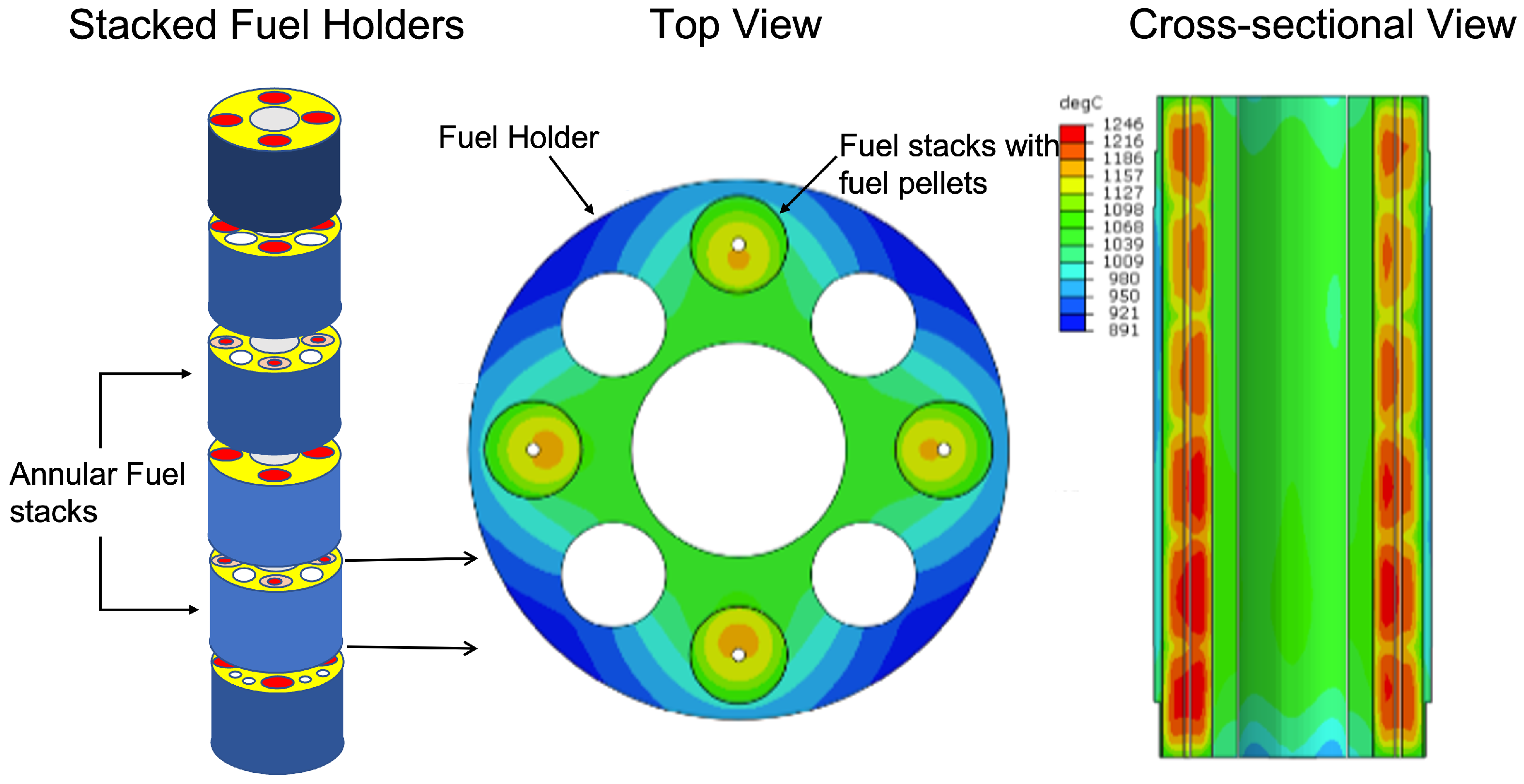
This case study will optimize thermocouple locations for accurately predicting the TRISO fuel temperature for an irradiation experiment being placed in the north–east flux trap of the advanced test reactor (ATR) at Idaho National Laboratory (INL). The algorithms are modular and agnostic with regard to the choice of fuel type, with the demonstration focused on TRISO fuel for the availability of data and models from ongoing projects at INL. The experiment comprises several capsules, each of which is equipped with its own temperature control and fission gas monitoring systems. The temperature control is achieved by real-time temperature measurement using TCs and through the flow of different composition gas blends (a helium–neon mixture) for temperature adjustment. To ensure independent temperature control for each capsule, a stainless steel wall pressure boundary and bottom and top caps are used for physical separation. Two types of fuel pellets are irradiated: solid and annular. The purpose of irradiating annular fuel is to obtain accurate temperature measurements as the solid fuel does not allow for TC penetration. Fuel temperature must be derived from the surrounding graphite-holder temperature measurement. If the TC positions in the holder are optimal, fuel temperature can be traced accurately. The annular fuel TCs then serve another function: a comparison of the derived and measured fuel temperatures. Figure 2 shows the cross-section of one of the annular fuel capsules. In the capsule, TCs are inserted into the graphite holder or the center hole of the annular fuel.

The capsule wall has a uniform inner diameter larger than the holder, thus leaving a convective heat gap between the holder and the capsule. The desired temperature of the fuel is achieved by adjusting the gap size. The convection influence on the fuel temperature evaluation has been investigated by a STAR-CCM+ 2210 (17.06.008-R8) simulation using a 2.54 mm (a bounding size that will not be exceeded) gap. As the temperature difference with or without convection is less than 1 K, without convective heat transfer, the experiment can be modeled by Abaqus 2021, a finite element code. The fuel generates both neutron and gamma heating while the non-fuel parts generate only gamma heating. Analyses of these heating regimes are obtained by the reactor physics analysis. Forced convection cooling outside the capsule wall is simulated through a convective (Neumann) boundary condition. The gas gap is affected by the holder and capsule thermal expansions, and irradiation induces graphite dimensional change. The in situ influence has been considered in the GAPCON subroutine of Abaqus. After obtaining the temperature field, these data are utilized to determine the optimal radial and axial coordinates for thermocouples, ensuring that they are constrained within the holder to accurately reconstruct the fuel temperature.

2.1.2. Lumped-Parameter Model of OPTI-TWIST

The OPTI-TWIST (Out-of-Pile Testing and Instrumentation Transient Water Irradiation System) is an electrically heated system to prototype TWIST, a nuclear fuel test vehicle. OPTI-TWIST tests instrumentation that is used to qualify nuclear fuel under accident scenarios, like a loss-of-coolant accident (LOCA) or a reactivity insertion accident. Monitoring temperature through optimally placed TCs in OPTI-TWIST eliminates complications of irradiation effects while preserving extreme thermal-hydraulic conditions. A lumped-parameter code, the Reactor Excursion and Leak Analysis Program (RELAP5-3D) [43], was used to model the system’s thermal-hydraulic parameters under transient operation.

Figure 3 shows the RELAP nodalization of OPTI-TWIST. The system is made up of two cylindrical pressure vessels connected by a quick-acting blowdown valve to simulate a break in a LOCA. The model assumes axis-symmetric conditions. Hydrodynamic volumes capture the fluid parameters at various elevations, while heat structures represent the solid internal and external walls. The electric surrogate fuel rod is seen to be vertically discretized but also radially discretized to represent the larger thermal gradients present. Spatial constraints are imposed on sensor placement in the heater region due to restrictions on the number of TCs that can be placed within the compact heater. Data that capture the evolution of thermal gradients through the transient can be used to determine constrained TC locations.

2.1.3. Instrumentation for TRISO Fuel Irradiation and OPTI-TWIST

Certain locations in the TRISO fuel experiment can reach temperatures up to 1500 °C. To withstand these conditions, high-temperature irradiation-resistant thermocouples (HTIR-TCs) made from molybdenum/niobium thermoelements have been developed at Idaho National Laboratory (INL), as shown in Figure 4. Monitoring the temperature of TRISO fuel over extended periods of irradiation is challenging due to thermocouple drift. Therefore, it is crucial to optimize the placement of these sensors to minimize uncertainty and maximize accuracy.

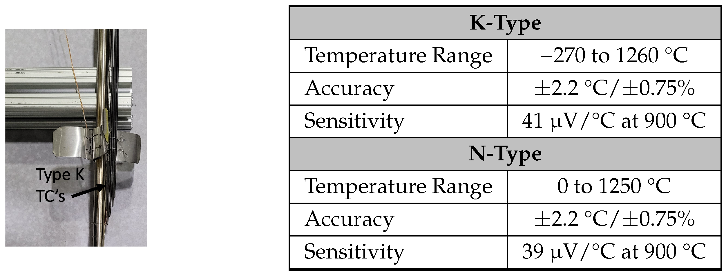
Conversely, K- and N-type thermocouples are commonly used for sensing in OPTI-TWIST, steam generators, and reactor vessels (Figure 5). While type K is the older standard, type N was specifically designed to withstand the irradiation in nuclear environments. With an accuracy of ±0.75%, it is essential to minimize errors and uncertainties arising from sensor reconstructions.

2.2. Modeling and Simulation for Steam Generators

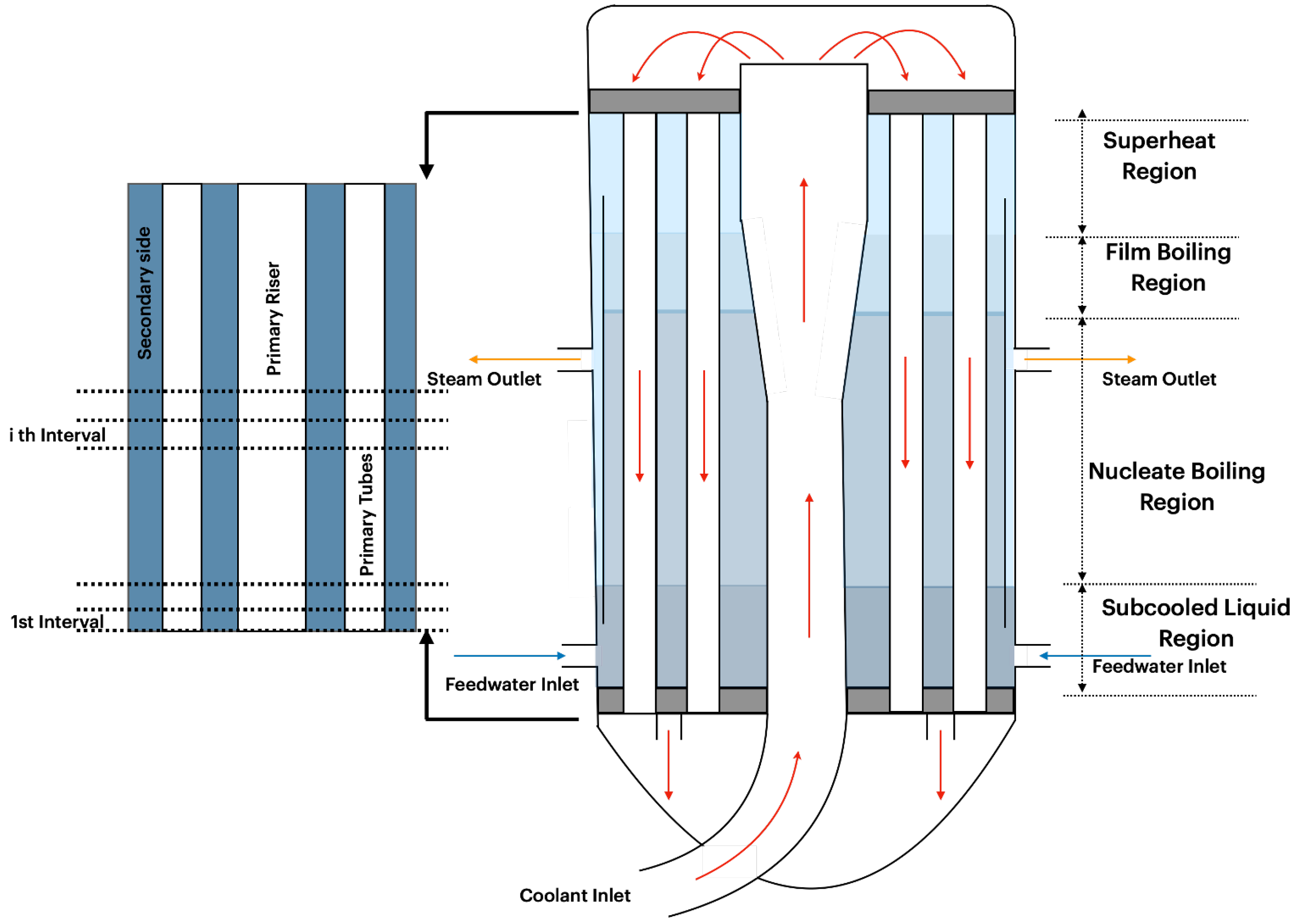
As the reactor coolant is heated due to the nuclear reaction, it enters the steam generator through the riser on the primary side. After a 180° turn, the coolant enters the primary tubes as shown in Figure 6. The heat transfer between the primary fluid to the secondary fluid takes place inside the shell through the walls of the tubes. The water temperature in the shell rises until it reaches saturation temperature and steam is produced, which then drives the turbine to produce electricity, as demonstrated in Figure 1. The secondary-side temperature, heat flux in the primary tubes which drives the conversion of water to steam, and the pressures on the primary and secondary sides are some fields of interest which determine control procedures for the nuclear power plants. As CFD modeling of the phase change phenomenon is challenging, we first explore a 1D model of the SG that simulates boiling. Next, we consider 3D CFD models with increasing complexity but with no phase change for sensor placement.

2.2.1. One-Dimensional Python Model of Steam Generator

Investigation of the thermal–hydraulic performance of the steam generator is essential for normal reactor operations and reactor safety during transients. Modeling and analyzing the single-phase liquid water flow (natural circulation) on the primary side and single-phase liquid water flow, subcooled boiling, saturated nucleate boiling, dispersed flow film boiling, and single-phase vapor/steam flow on the secondary side, and the transition between these flow regimes is essential in predicting the SG performance. A Python code which uses 1D grids to discretize the long SG tubes into thousands of intervals and model phase transition regimes along the SG height is developed for the thermal–hydraulic analysis of a vertical shell once-through steam generator (OTSG) for a PWR.

The code starts the calculation from the bottom of the SG (first computational node), with an initial guess of the primary-side outlet temperature. Through these known fluid properties, the boundary conditions for the second interval and the SG’s overall heat transfer coefficient can be calculated from the effectiveness-NTU method. After looping through all computational nodes/intervals, the primary-side inlet temperature can be obtained and the subsequent convergence criterion depends on the difference between the computed value and the input parameter. The monitoring of the phase transition within the steam generator tubes through optimal locations of TCs, pressure taps, and heat flux sensors along the height of the SG while considering spatial constraints is enabled through this 1D code.

2.2.2. Three-Dimensional CFD Model of Steam Generator

The previous 1D models nodalized and oversimplified fluid flow in the SG to 1D flow paths, and the sensor locations could only be determined along the height. Computational fluid dynamics (CFD) models in 3D are superior to their 1D counterparts in capturing the spatial distribution of velocity, pressure, and other fluid properties throughout the entire domain. This results in a more precise and detailed sensor optimization that captures flow phenomena such as turbulence, boundary layer effects, and fluid interactions with solid boundaries. Monitoring the flow distribution in the upper shell/plenum of the SG plays a critical role in predicting and preventing potential accidents that could jeopardize the structural integrity of the nuclear reactor. While multiple sensors can be mounted in the region of interest, they can impact the flow distribution and lead to high costs. Temperature distribution within the primary riser and secondary tubes is another field of interest captured through thermocouples. For temperature measurements, one of the SG tubes can be replaced with an instrumented tube. Ideally, multiple temperature measurements can be performed along the SG tube. However, the space available for the probes is constrained by the tube size and only a few sensors can be placed along it. Minimizing the number of sensors and strategically placing them to capture the data required to provide insights into the flow distribution and thermal gradients are necessary.

Due to the large size of the SG, the geometry was simplified by excluding the shell’s walls, baffles, lower head, etc. Instead, only the fluid volume of the upper shell, 1.828 m (72 inches) of the riser’s length, and partial tube length (1.828 m) are modeled. The geometry’s fluid domain is further reduced by modeling only a quarter of the steam generator, as illustrated in Figure 7, to reduce the computational cost of the CFD models. Figure 7 summarizes the dimensions used to generate the CAD model.

The geometry is discretized using a polyhedral mesh, as illustrated in Figure 8. The inlet has a mass flow rate boundary condition, while the tubes have a pressure outlet boundary condition. For purposes of this analysis, an adiabatic boundary condition is imposed on the outer walls of the upper shell. However, a convection boundary condition is assigned to the riser and tubes. A summary of the assumed boundary conditions is presented in Figure 8 along with the mesh settings.

2.2.3. Instrumentation for Steam Generators

The Sporian ThermaFlow™ 700 sensor, refer to Figure 9, manufactured by Sporian Microsystems Inc. in Lafayette, CO, USA, is a velocity probe that can withstand the operating conditions of the SG. Its length can be manufactured according to user requirements and it is used to monitor flow distribution. The probe can perform both velocity and temperature measurements, and its technical specifications are summarized in Figure 9. An instrumentation port can be machined in the upper plenum for the sensor. The K- and N-type thermocouples (Figure 5) in the previous section are also used for temperature measurements within the SG. Pressure taps and fiber-optic sensors can be placed within SG tubes and shell to provide localized measurements (Figure 10). Heat flux can be measured through small square sensors that are mounted to the outer and/or inner surface of the SG wall (Figure 11).

2.3. Constrained Sensor Placement for Reconstruction

The proposed sensor placement methodology can be summarized in few simple steps. First, a high-fidelity code (e.g., Star-CCM+ for CFD, ABAQUS for structural mechanics, or RELAP5-3D for reactor thermal–hydraulics) is used to create a large data cloud by perturbing the problem’s parameters. The data are then split into a training set and a testing set. The training data are then used to extract a proper reduced basis that best describes/fits the data. Next, a greedy algorithm based on QR factorization with column pivoting is used to approximate the optimal solution to the reconstruction problem and avoid solving the combinatorial exhaustive search. The pivoting process rearranges the columns such that the leading columns reflect the most important points in the discretized grid which are in turn, the optimal sensor locations. Finally, the testing set is used to validate the reconstructed field based on the sparse measurements in the optimal locations. The key performance indicator (KPI) and validation metric in this case is the relative error in the reconstructed signal from sparse measurements relative to the high-fidelity simulation. The detailed mathematics is outlined below. In nuclear capsules and steam generators, the number of locations available for sensor measurements is extremely limited compared to the high-dimensional latent flow fields that need reconstruction. However, most nuclear processes are governed by a smaller set of underlying physical principles. Reduced-order models (ROMs), such as proper orthogonal decomposition (POD), enable sparse sensing by providing a minimal rank approximation of data ($\mathbf{X}$) from high-fidelity simulations through a singular-value decomposition (SVD) of data snapshots $\mathbf{X}=\mathsf{\Psi }\mathbf{D}{\mathbf{V}}^{*}$. This approach represents high-dimensional system states $\mathbf{x}\in {\mathbb{R}}^n$ as a truncated linear combination of the leading r POD modes:

$$\mathbf{x}={\mathsf{\Psi }}_r\mathbf{a},$$

where $\mathbf{a}$ is a low-dimensional vector of mode coefficients, facilitating sparse sensing reconstruction. The problem then reduces to estimating $\mathbf{a}$ from sparse measurement data.

Each case study is analyzed using optimal sensor placement with uncertainty developed in our previous work [41,42], summarized next. The reconstruction setup encodes sensor placement as a sparse measurement operator of high-dimensional system states, where the resulting vector of p measurements ($\mathbf{y}\in {\mathbb{R}}^n$) can contain additive zero-mean Gaussian noise $\eta \sim \mathcal{N}(\mathbf{0},{\beta }^2)$:

$$\mathbf{y}=\mathbb{S}\mathbf{x}+\mathit{\eta }.$$

(1)

The measurement selection operator $\mathbb{S}\in {\mathbb{R}}^{p\times n}$ is designed to select p maximally informative sensor measurements of the full state $\mathbf{x}$. The desired selection operator $\mathbb{S}$ is a sparse matrix containing canonical basis vectors ${\mathbf{e}}_j$ for ${\mathbb{R}}^n$ with a unit entry where a sensor is selected and zeros everywhere else. The vector $\mathbb{S}\mathbf{x}$ represents locations of the state that are chosen to be measured. By substituting the POD representation of the unknown state, the full state is reconstructed using the Moore–Penrose pseudoinverse of the product $\mathsf{\Theta }=\mathbb{S}{\mathsf{\Psi }}_r$, known as Gappy POD [46]:

$$\begin{array}{ccc}\hfill \mathbf{y}& =\mathbb{S}{\mathsf{\Psi }}_r\mathbf{a}+\mathit{\eta }\hfill & \hfill =\mathsf{\Theta }\mathbf{a}+\mathit{\eta }\\ \hfill \widehat{\mathbf{x}}& ={\mathsf{\Psi }}_r{\left(\mathbb{S}{\mathsf{\Psi }}_r\right)}^{†}\mathbf{y}\hfill & \hfill ={\mathsf{\Psi }}_r{\mathsf{\Theta }}^{†}\mathbf{y}.\end{array}$$

(2)

The optimal sensors are row indices of ${\mathsf{\Psi }}_r$ that condition the matrix inversion to enable the best reconstruction of $\widehat{\mathbf{x}}$. The developed methodology minimizes error covariance $\mathsf{\Sigma }$ between the true state and reconstructions from noisy measurements

$$\mathsf{\Sigma }=\mathrm{Var}(\mathbf{a}-\widehat{\mathbf{a}})={\beta }^2{\left({\mathsf{\Theta }}^T\mathsf{\Theta }\right)}^{-1}$$

(3)

using D-optimal design criteria. Given a budget of p sensors, this statistical metric aims to capture maximum information volume by maximizing the determinant of the Fisher information of the measurements [47], ${\mathsf{\Theta }}^T\mathsf{\Theta }$. Maximizing the logarithm of this criterion also results in a selection of an optimized sensor set:

$${\gamma }_{*}=arg\underset{\gamma ,\left|\gamma \right|=p}{max}logdet\left({\mathsf{\Theta }}^T\mathsf{\Theta }\right).$$

(4)

Brute-force optimization over $\gamma$ scales combinatorially with the number of candidate locations and is therefore intractable. We develop a greedy strategy based on QR factorization with column pivoting that decomposes a matrix $\mathbf{W}\in {\mathbb{R}}^{m\times n}$ into a unitary matrix $\mathbf{Q}$, an upper-triangular matrix $\mathbf{R}$, and a column permutation matrix $\mathsf{\Pi }$, such that $\mathbf{W}\mathsf{\Pi }=\mathbf{Q}\mathbf{R}$. QR pivoting is applied to ${\mathsf{\Psi }}_r^T$ and the permutation matrix keeps track of the selected sensors. A partial QR factorization step in the pivoting procedure can be shown as

$$\mathbf{W}\mathsf{\Pi }=\mathbf{Q}\mathbf{R}=\mathbf{Q}\left[\begin{array}{cc}{\mathbf{R}}_{11}^{\left(k\right)}& {\mathbf{R}}_{12}^{\left(k\right)}\\ 0& {\mathbf{R}}_{22}^{\left(k\right)}\end{array}\right],$$

(5)

where $\mathbf{Q}\in {\mathbb{R}}^{m\times m}$ is orthogonal, ${\mathbf{R}}_{11}^{\left(k\right)}\in {\mathbb{R}}^{k\times k}$ is upper-triangular, ${\mathbf{R}}_{12}^{\left(k\right)}\in {\mathbb{R}}^{k\times (n-k)}$, ${\mathbf{R}}_{22}^{\left(k\right)}\in {\mathbb{R}}^{(m-k)\times (n-k)}$, and $\mathsf{\Pi }\in {\mathbb{R}}^{n\times n}$ is the permutation matrix containing information about the first k chosen sensors [39,48,49]. Having selected k sensors, the ${(k+1)}^{st}$ is chosen by selecting a column from submatrix ${\mathbf{R}}_{22}^{\left(k\right)}$ that has the maximal two-norm.

Constraints are introduced while choosing the next iterate by forcing the selected pivot column to lie within allowable column indices based on the constraints applied [42]. The algorithm handles region constraints where exactly or a maximum of s sensors are allowed in a particular constraint region and the remaining $r-s$ must be outside it. It can handle cases where a certain number of sensor locations s are predetermined and the remaining $r-s$ need to be optimized or adaptive distance constraints, where sensors must be located at a specific distance d apart from each other. These constraints are implemented in the final $r-s$ steps of the QR pivoting procedure, so as to allow upper triangularization of the first few terms of $\mathbf{R}$ to proceed normally [42]. Thus, allowing the best sensors to be chosen in allowable regions at each iteration is the key driver of reconstruction accuracy. We evaluate the reconstruction accuracy through the relative reconstruction error ($ϵ$), where

$$\mathrm{relative}\mathrm{reconstruction}\mathrm{error}\left(ϵ\right)=\frac{\parallel \mathbf{x}-{\mathsf{\Psi }}_r{\left(\mathbb{S}{\mathsf{\Psi }}_r\right)}^{†}{\mathbf{y}\parallel }_2}{{\parallel \mathbf{x}\parallel }_2}\times 100.$$

(6)

Sensor measurements often contain noise levels that contribute to reconstruction errors. Noisy sensor readings of pressure, velocity, and temperature within nuclear fuel and steam generators can lead to critical safety risks for the entire nuclear power plant. To quantify the uncertainty in the reconstructed state in the presence of noise, previous work [41] estimates the expected state covariance for a regularized Gappy estimator. The standard deviation in the reconstruction of each grid point is calculated from the diagonal of the estimated error covariance matrix:

$$\begin{array}{cc}\hfill \mathbb{E}[\Delta \widehat{\mathbf{x}}\Delta {\widehat{\mathbf{x}}}^T]& ={\mathsf{\Psi }}_r\frac{{\mathsf{\Sigma }}^{-1}}{{\beta }^2}{\mathsf{\Theta }}^T\mathbb{E}[\Delta y\Delta y^T]\mathsf{\Theta }\frac{{\mathsf{\Sigma }}^{-1}}{{\beta }^2}{\mathsf{\Psi }}_r^T,\hfill \end{array}$$

(7)

$${\sigma }_i=\beta \sqrt{\sum _j{\left({\mathbf{F}}_{ij}\right)}^2}\mathrm{where}\mathbf{F}\equiv {\mathsf{\Psi }}_r{\mathsf{\Sigma }}^{-1}\frac{{\mathsf{\Theta }}^T}{{\beta }^2}.$$

(8)

To inform the recalibration of DT models and to predict when sensor measurements are corrupted by noise, $3\sigma$ standard deviation bounds computed from the diagonal entries of the covariance matrix ${\mathsf{\Sigma }}_{\mathit{i}\mathit{i}}$ can be a useful metric to quantify uncertainty in the reconstruction errors $\mathbf{a}-\widehat{\mathbf{a}}$. However, true sensor measurements $\mathbf{a}$ are required for this uncertainty estimate. When true coefficients are unavailable, a statistical analysis of the distribution of each estimated coefficient $\widehat{\mathbf{a}}$ provides metrics for detecting the divergence of sensor readings from expected values. The expected mean ${\mu }_i=\mathbb{E}\left[{\widehat{\mathbf{a}}}_i\right]$, covariance, and standard deviation of the distributions of estimated POD coefficients are computed using

$$\mathbb{E}\left[{\widehat{\mathbf{a}}}_i\right]={\mathsf{\Sigma }}^{-1}\frac{{\mathsf{\Theta }}^T}{{\beta }^2}\mathbb{E}\left[{\mathbf{y}}_i\right]$$

(9)

$$\begin{array}{c}\hfill \mathbb{E}[\Delta \widehat{\mathbf{a}}\Delta {\widehat{\mathbf{a}}}^T]=\frac{{\mathsf{\Sigma }}^{-1}}{{\beta }^2}{\mathsf{\Theta }}^T\mathbb{E}[\Delta y\Delta y^T]\mathsf{\Theta }\frac{{\mathsf{\Sigma }}^{-1}}{{\beta }^2}.\end{array}$$

(10)

$${\sigma }_i=\beta \sqrt{\sum _j{\left({\mathbf{T}}_{ij}\right)}^2}\mathrm{where}\mathbf{T}\equiv {\mathsf{\Sigma }}^{-1}\frac{{\mathsf{\Theta }}^T}{{\beta }^2}.$$

(11)

We extend the methodology developed in [42] to locate sensors for estimating mass flow rates and other parameters in steam generator models. These sensor placements minimize reconstruction errors, provide statistical bounds for noise-induced uncertainties, and initiate two-way communication between the physical components of an NPP and the DT.

2.4. Uncertainty Estimation in Digital Twins

Uncertainty can originate extrinsically such as uncertain inputs to a model, user-introduced errors, truncation errors, and misinterpretations. This is usually referred to as epistemic uncertainties for they can be reduced by acquiring more knowledge, adding more terms to the truncated model, or acquiring more data/samples. Uncertainty can also originate intrinsically such as inherent stochasticity, noisy telemetry data, low-resolution images, and instrumental uncertainty. This is usually referred to as aleatoric uncertainty because it cannot be reduced since it usually incorporates random probabilistic natures. In nuclear applications, the separation between these types of uncertainties is imperative for its tight coupling to safety and regulatory aspects [50], which explains significant investments to integrate covariance cross-section data in nuclear codes such as SCALE.

Uncertainty in digital twin (DT) predictions propagates from sensor noise, upstream process disturbances, and modeling errors. This uncertainty, originating in the precision and noise of sensor measurements, cascades through DT subsystem components. Uncertainty quantification is crucial for verifying predicted temperatures, heat flux, and flow components within nuclear reactors. In this study, we design sensor placements to systematically minimize and characterize uncertainty from sensor-based state reconstruction in digital twin components, utilizing low-dimensional representations of simulation data.

3. Results

This section illustrates the optimization of sensors for reconstructing key fields within the reactor and steam generator subsystems of the NPP. We account for various constraints arising from working conditions, manufacturing considerations, and spatial limitations during optimization. Our focus lies on reconstructing temperature, pressure, velocity, and heat flux within a steam generator, a TRISO fuel irradiation experiment, and an electrically heated fuel rod prototype capsule (OPTI-TWIST), using thermocouples, pressure taps, velocity probes, and heat flux sensors as described in Section 2. We achieve minimal error in reconstructing the target response compared to randomly selected sensor locations and conduct uncertainty analysis on noisy measurements to flag recalibration of digital twin models.

3.1. One-Dimensional Steam Generator Model

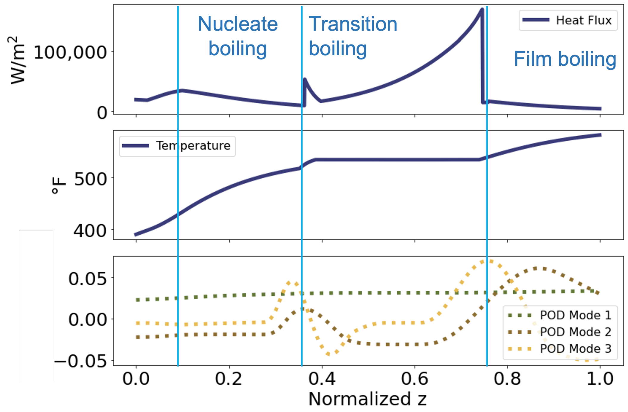
The 1D steam generator (SG) model, described in Section 2.2.1, offers a computationally efficient alternative to more complex computational fluid dynamics (CFD) solvers. This model is particularly useful for estimating key parameters such as temperature, heat flux, and pressure within the steam generator. The model helps to estimate secondary-side temperature, especially during the phase transition of water to steam. Temperature measurements are typically obtained using K- and N-type thermocouples (TCs) (Figure 5), which provide point-wise temperature readings. On the secondary side, the steam generator tubes are supported by 42 baffles evenly distributed along their length. These baffles maintain tube positioning during assembly and prevent vibration from flow-induced eddies during operation. Sensor placement is constrained by the need to avoid these baffles. The sensor placement algorithm is trained on 442 steady-state samples of secondary-side temperature to determine optimal sensor locations while accounting for baffle constraints. Using p = 3 sensors, the field of interest is reconstructed for one test sample, achieving a maximum reconstruction error ($ϵ$) of 0.9% compared to the ground truth (Figure 12). In the presence of noisy sensor measurements, state reconstruction uncertainty is low along the height of the SG with a maximum of 0.01 °F (Figure 12). Below $z=0.4$, the temperature of water rises and remains constant between $z=0.4$ and $z=0.8$ due to phase change from water to steam. Across the entire test set (162 samples), the maximum reconstruction error is 0.9% for QR-selected sensors compared to ($ϵ$ = 6.4%) for randomly placed sensors.

The relationship between the secondary-side temperature and heat flux ($\dot{\mathbf{Q}}$) in the steam generator tubes was further analyzed. Optimized temperature sensors capture energy fluctuations in the POD modes. The leading POD mode represents the overall temperature profile, and the second and third modes capture the heat flux that causes the temperature variation (Figure 13). Heat flux, dependent on temperature gradients, can be estimated from TC-based temperature reconstructions outside the phase change region $z\in [0.4,0.8]$. During phase change, temperature gradients vanish, and the heat flux is determined by the latent heat coefficient and the mass of the substance undergoing phase change. Heat flux for the different boiling regions is calculated separately, resulting in abrupt changes between boiling regimes. Further analysis of time-dependent data can allow for the inference of heat flux from temperature measurements.

Currently, the algorithm is trained on 442 steady-state samples of heat flux in the tubes and shell for locating baffle-constrained optimal sensors. Heat flux can be measured using small square sensors attached to the steam generator’s outer/inner wall (Figure 11). The highest reconstruction error over all samples compared to the ground truth is $ϵ$ = 20.6% for QR-selected sensors (Figure 12). The higher error is due to modeling discontinuities in the training data for heat flux across different boiling regimes. Experimentally, heat flux decreases gradually after the phase change, as shown by sensor-based reconstructions, in contrast with the abrupt decrease caused by modeling discontinuities. For randomly placed sensors, the maximum error rises to $ϵ$ = 48.9%. Under noisy sensor measurements, state reconstruction uncertainty is low for QR-optimized sensors along the height of the SG with a maximum of 0.0099 W/m² (Figure 12).

Another important field of interest is secondary-side pressure, measured locally with pressure taps on the steam generator shell (Figure 10). Due to the low pressure variation (≈0.04 MPa), QR-selected sensors reconstruct the field with very high accuracy, achieving a maximum reconstruction error of $ϵ=0.002\%$ across all test samples (Figure 12). In contrast, randomly placed sensors fail to capture these small variations in pressure, resulting in a maximum error of $ϵ=1\%$ (Figure 12). The maximum noise-induced uncertainty in pressure reconstruction is also low (0.009 MPa). Additionally, there is a linear relationship between secondary- and primary-side pressures, allowing regression techniques to infer one field from measurements of the other.

In conclusion, 3D CFD modeling of phase change phenomena is computationally expensive for complex systems such as steam generators. Using 1D nodalization provides an efficient alternative, offering real-time updates of multiple fields of interest. Optimized sensor locations derived from 1D modeling data can help uncover the underlying physics of boiling regimes to estimate preliminary errors and uncertainties, aiding in the development of control regimes through digital twinning. Despite the advantages of 1D models, it is crucial to instrument specific tubes and place sensors in a 3D coordinate system. For licensing and safe operations, measuring flow distribution within the shell and tubes is essential. The next section explores a 3D model of the steam generator for optimizing temperature and velocity sensors.

Three-Dimensional Steam Generator Model

This section applies the sensor placement methodology to a 3D CFD model of the steam generator described in Section 2.2.2. The mass flow rate $\left(\dot{m}\right)$ kg/s of the primary coolant varies between $\dot{m}\in [0.1,3]$ and $\delta \dot{m}=0.1$. As the mass flow rate increases, the temperature variation ($\Delta T=T_{maximum}-T_{minimum}$) decreases, given a constant heat flux boundary condition. Temperature measurements can be taken using K- or N-type point TCs or the Sporian ThermaFlow sensors described in Section 2.2.3. These sensors can be placed within the shell, riser, and tubes of the SG. It is easier to place sensors in the shell as compared to the tubes and riser, as the flow within these narrow cylindrical bodies can be obstructed due to sensors. Instrumenting one tube or just the riser reduces sensor costs and allows for normal flow development in the remaining tubes. The objective of optimizing sensor locations is to limit instrumentation to lie either within the shell or to just one of the tubes.

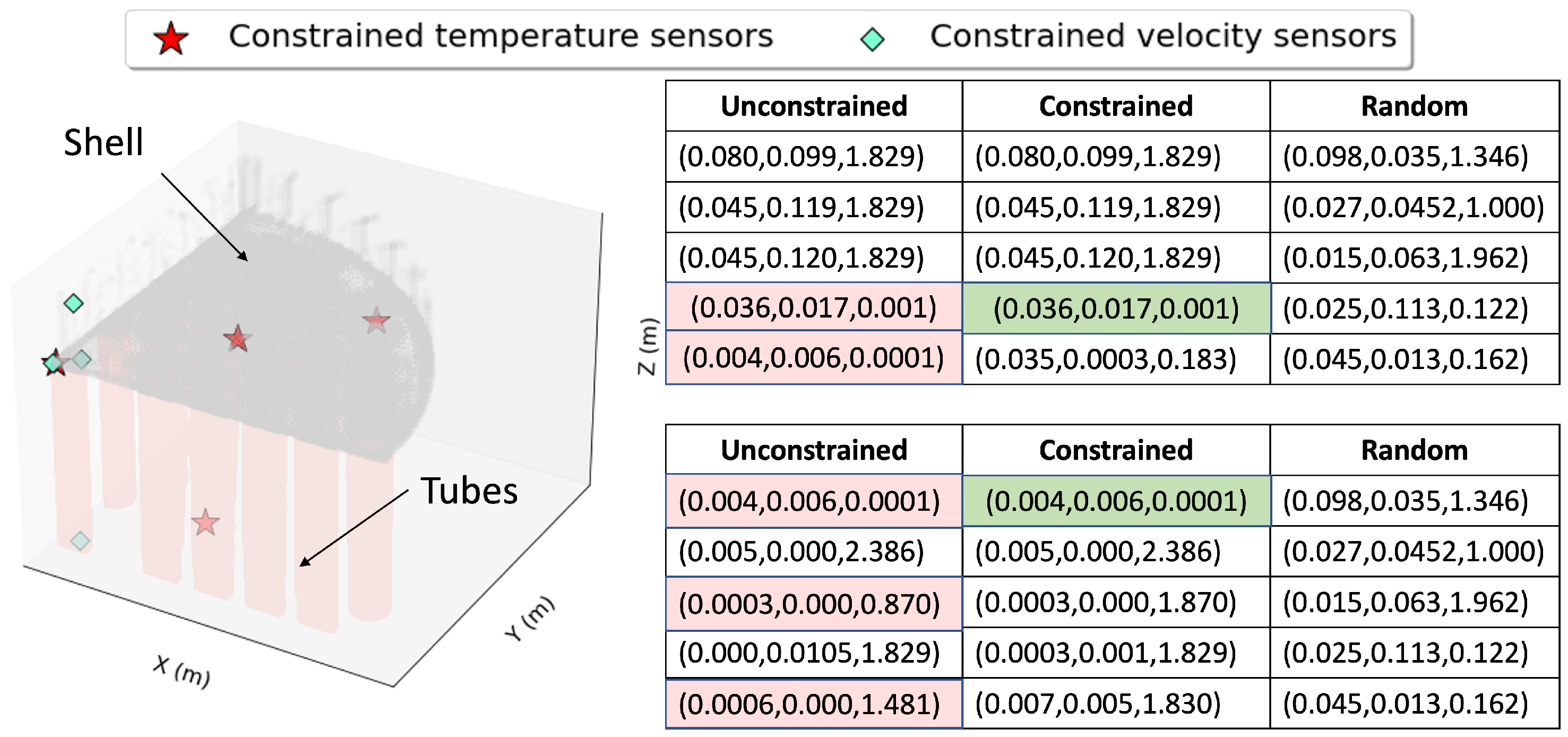
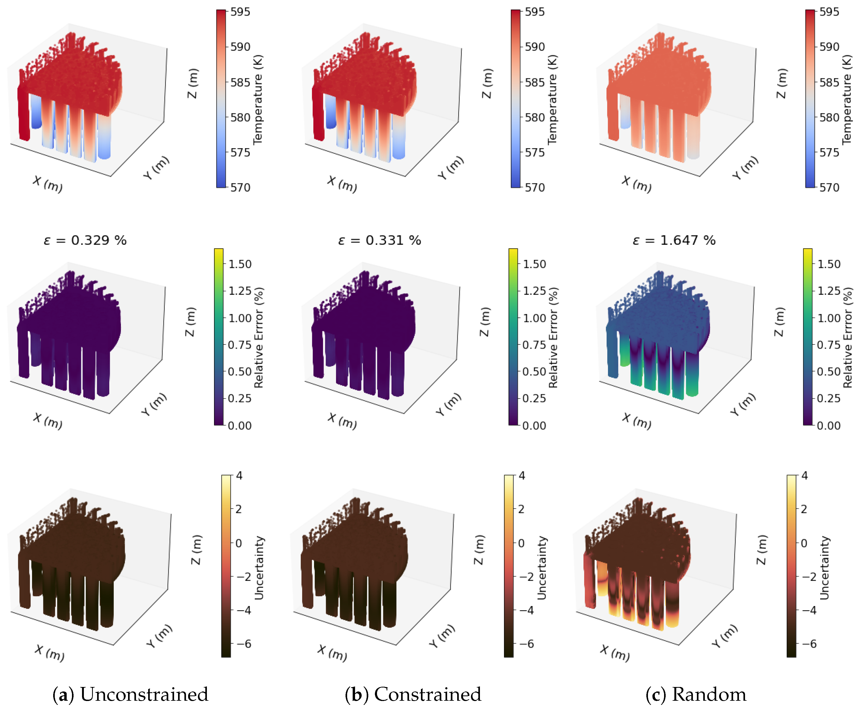
Optimized, unconstrained QR pivoting locates two sensors in the SG tubes (z < 1.828 m in Figure 14) and achieves a reconstruction error of $ϵ=0.329\%$. In contrast, constrained optimization places only one sensor in the tube while maintaining a comparable reconstruction error of $ϵ=0.331\%$ (Figure 15a,b). Optimal sensor reconstructions outperform randomly placed sensor reconstructions which have a maximum error of $ϵ=1.647\%$ (Figure 15c). In these figures, we reconstruct temperature profiles developed by the nominal mass flow rate $\dot{m}$ = 1.2 m/s. Additionally, reconstruction errors decrease with increasing mass flow rate (Figure 16) due to reduced temperature variation at higher mass flow rates (brown dots in Figure 16). Ensembles of randomly located sensors (error bars in Figure 16) fail to accurately capture the temperature field across the SG. A similar trend is observed in noise-induced uncertainties, with QR-optimized sensors showing a maximum uncertainty of 0.010 °K, while random sensor placements result in uncertainties up to 20% (as shown in row 3 of Figure 15a–c).

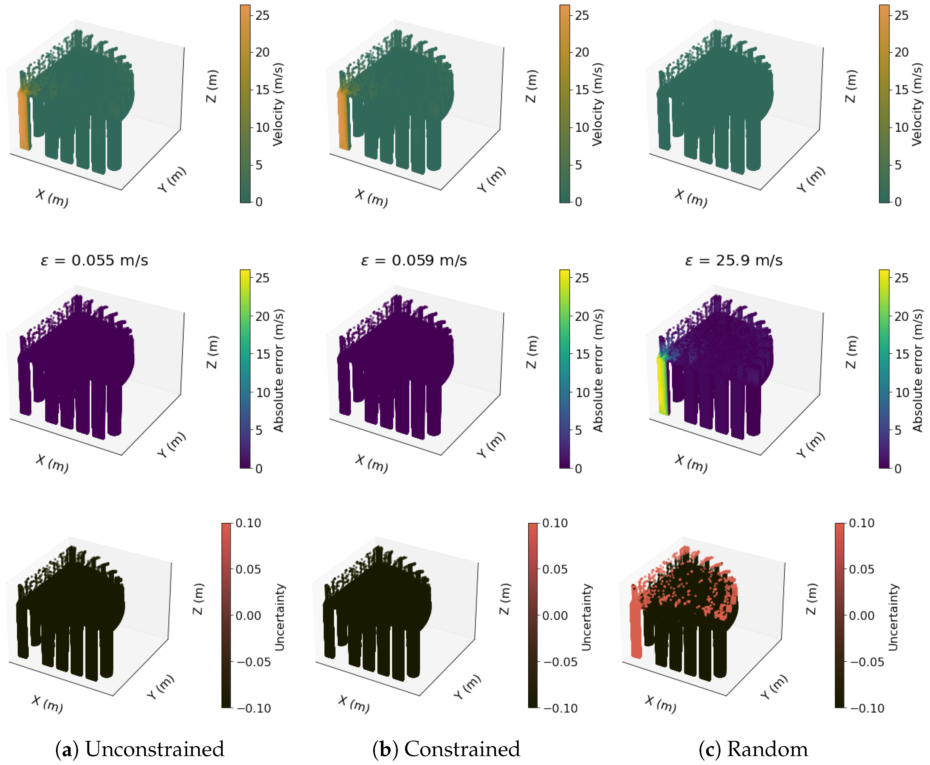
Next, the algorithm was applied to velocity data of the 3D SG as the coolant flows through the riser, makes a 180° turn through the shell, and returns to the tubes. Measuring the distribution of coolant entering the various tubes is crucial for manufacturing and can be achieved using Sporian ThermaFlow sensors described in Section 2.2.3. Similar to TC placement, instrumenting just one tube is key to allowing for normal flow development in the others. Optimized unconstrained QR places three sensors among the tubes (z < 1.828 m in Figure 14), achieving a maximum absolute reconstruction error of 0.005 m/s and a maximum noise-induced uncertainty of 0.010 m/s (Figure 17a). With constraints, only one sensor is placed in the tubes, with the rest in the shell, resulting in a maximum absolute reconstruction error of 0.005 m/s and a comparable maximum uncertainty of 0.8 m/s (Figure 17b). Randomly placed sensors fail to reconstruct velocity accurately, and have a maximum absolute error of 25 m/s while uncertainty rises to ${10}^3$ m/s (Figure 17c). Across all mass flow rates, QR-optimized sensors maintain a low reconstruction error of 0.05 m/s, whereas random sensors exhibit high errors as indicated by the blue error plots (25 m/s) (Figure 18).

Unconstrained optimization favors locating sensors within the tube and riser due to the richer dynamics that exist there. Imposing sensor constraints within QR results in a near-optimal placement in the shell and one of the tubes, as well as a negligible loss of reconstruction performance. The 3D CFD model of the steam generator, comprising 5,616,200 mesh points, provides the velocity and temperature data. QR-optimized sensors can reconstruct these high-dimensional fields using just five sensors ($p=5$) with minimal errors, which enables real-time monitoring of the SG. On the other hand, the random placement of sensors within the SG introduce large errors and uncertainties. Therefore, placing sensors without optimizing them in regard to the underlying flow especially in the presence of noisy sensor measurements can introduce large errors in the corresponding digital twins. Informed planning of instrumentation for the steam generator can play a key role in real-time digital twinning, monitoring steam quality, flow distributions, and nominal working conditions while also preventing accidents and detecting anomalies.

3.2. Irradiation of TRISO Fuel

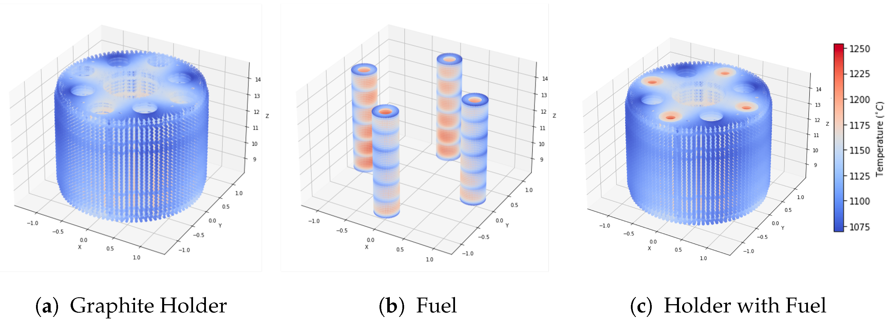
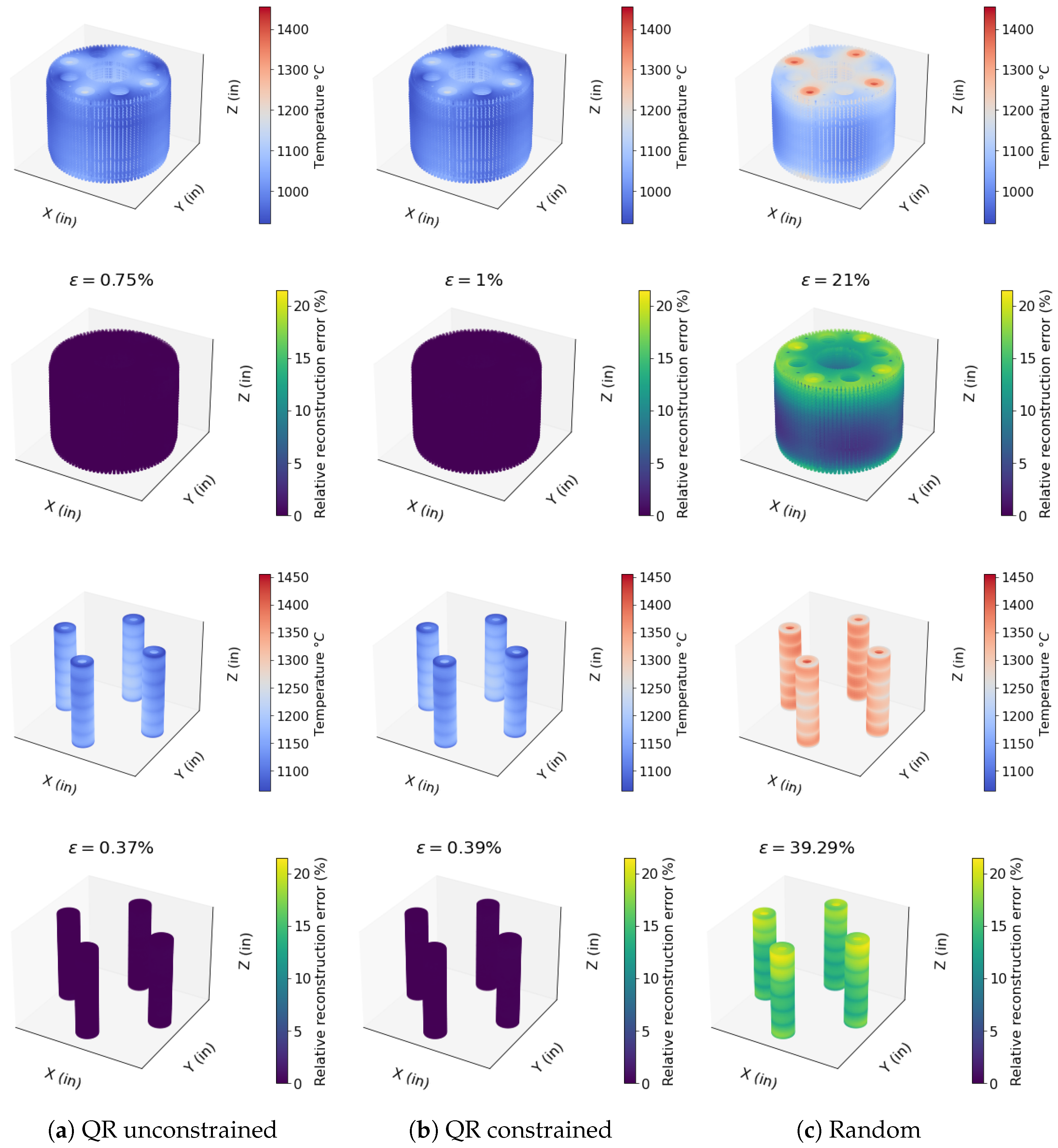
To support the next generation of reactors, testing, validation, and performance assessment of new fuels under reactor working conditions are essential. Monitoring TRISO fuel temperature (Figure 19a) during irradiation experiments is challenging due to the extreme temperatures (1200–1300 °C) inside the fuel. As detailed in Section 2.2.3, HTIR-TCs can withstand temperatures exceeding 1600 °C [51]. However, nuclear TCs eventually drift due to long-term exposure to neutron bombardment and high temperatures [52]. Placing sensors in the surrounding graphite holder (Figure 19b) allows for accurate temperature reconstruction within the fuel stacks, reducing TC exposure to high temperatures, minimizing drift and extending sensor lifespan.

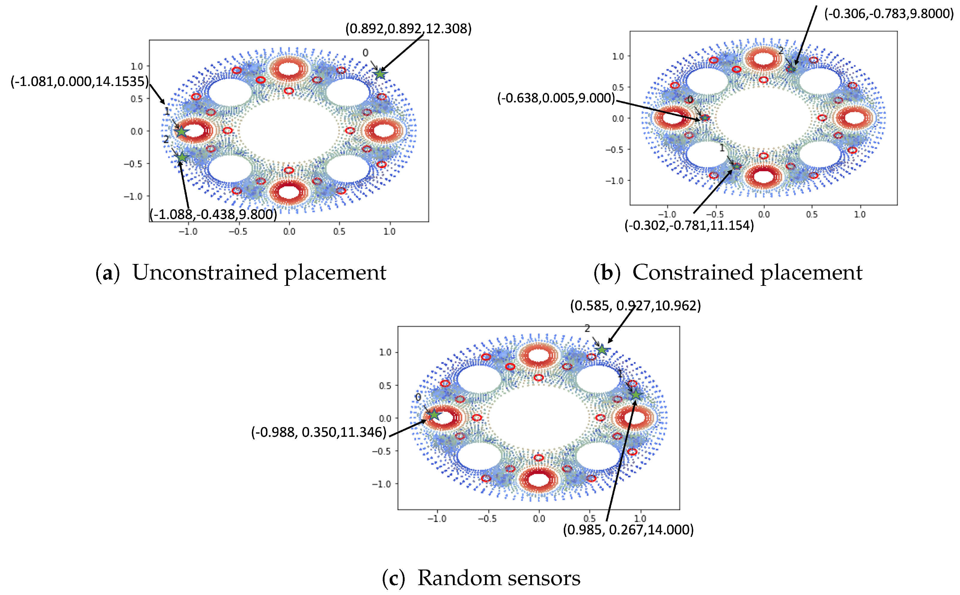
In the graphite holder, TCs cannot be placed at all locations due to constraints on drilling holes to accommodate sensors and inert gas inlets and outlets. Figure 20 illustrates available drilling locations for TCs (red circles). The developed sensor placement algorithm must select three to four holes from the given nineteen possibilities, with each hole accommodating just one sensor, while also determining the depth of the TC within the drilled holes. Data are derived from a 3D FEM model described in Section 2.1.1, representing the beginning (BOC) and end (EOC) of fuel irradiation cycle. Neutron and gamma heating information is obtained through reactor physics analysis, which is computationally intensive and time-consuming and can only provide 10 samples. The algorithm is trained using eight randomly selected samples of EOC and BOC data and tested on the remaining two samples.

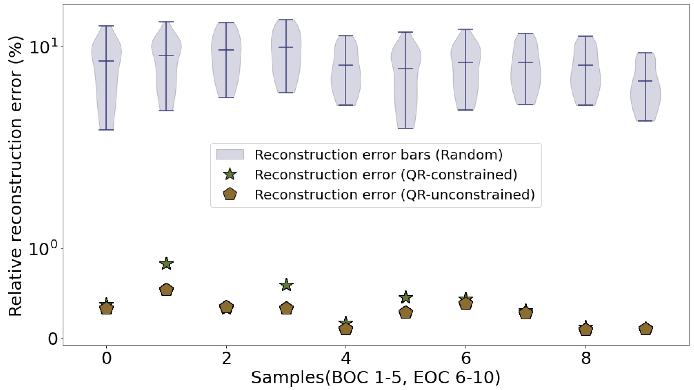
Optimized, unconstrained QR pivoting selects sensors strategically within the fuel and along the edges of the capsule to capture maximum temperature variance (Figure 20a). However, due to constraints on drill locations for TCs within the capsules, these unconstrained sensor placements are not feasible in a physical experiment. Thus, the developed algorithm constrains sensor optimization to points within the 19 possible drill locations (Figure 20b). Measurements at these constrained locations result in a maximum relative reconstruction error of $1\%$ (Figure 21b), whereas unconstrained reconstruction yields a maximum error of $ϵ=0.75\%$ (Figure 21a) for the entire capsule. Random sensor placement (Figure 20c) refers to intuitive selection based on the ease of maintenance and access, which leads to inaccurate reconstruction with higher errors $ϵ=25\%$ (Figure 21c). To illustrate various random selections of sensors, 20 ensembles of random unconstrained sensor combinations were used to reconstruct temperature profiles for all the samples. A comparison with QR-optimized sensors ($1\%$) shows higher reconstruction errors for random ensembles (30%) (Figure 22).

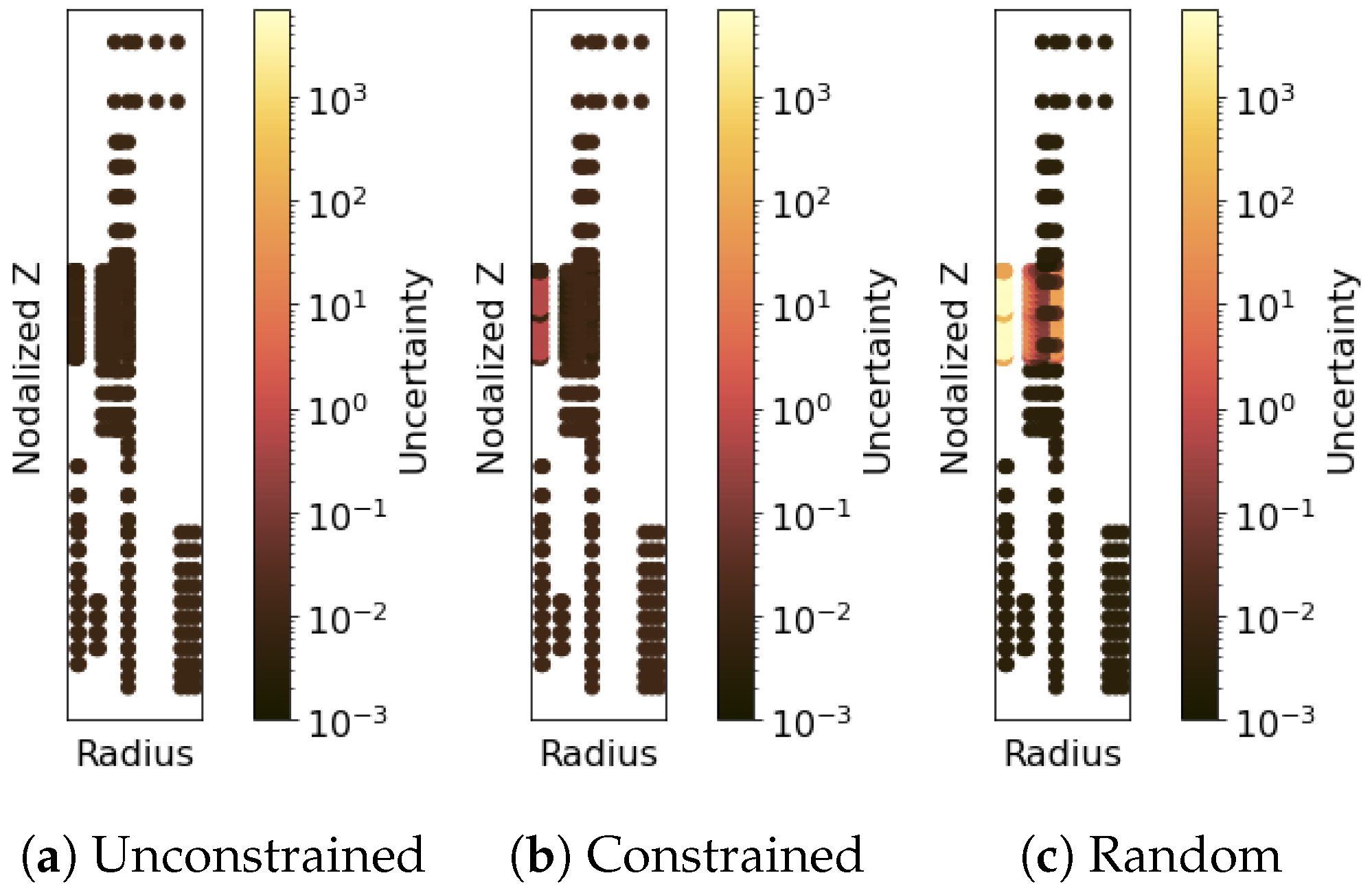
Zero-mean Gaussian noise with $\beta =0.01$ is added to analyze uncertainty heatmaps for temperature reconstruction to illustrate noisy TC readings as in Equation (7). The maximum uncertainty for constrained sensing is 0.0241 °C (Figure 23b) as compared to unconstrained sensor placement (Figure 23a), which has an uncertainty of 0.010 °C. Randomly placed sensors result in very high uncertainty for state reconstruction (9.8 °C) (Figure 23). In summary, the sensor placement framework accounts for design, manufacturing, and deployment constraints to optimize sensor placement. It provides error estimates and uncertainty for noisy sensor readings from modeling data, aiding in approximating errors in physical experiments and establishing manufacturing parameters such as drill hole depths for TCs. Accurate reconstructions and uncertainty bounds (Equation (10)) through sensors can help quantify TC drift due to long-term radiation exposure in TRISO fuel through digital twinning.

3.3. Electrically Heated Prototype Capsule- OPTI-TWIST

In this section, thermocouple (TC) locations are optimized for reconstructing temperature within an electrically heated fuel rod (OPTI-TWIST), simulating the behavior of a nuclear fuel rod as described in Section 2.1.2. Analyzing the impact of power transients on reactor core coolant temperature, pressure, and velocity is crucial for real-time safety monitoring and control in a nuclear reactor. In this study, sensor placements were optimized to capture heat flow dynamics during power transients. It is important to detect when sensor readings diverge from predicted metrics in the presence of noise during transients. This early detection can signal the need for digital twin recalibration and prevent accidents caused by power surges at a nuclear facility. In this case, the power surge is modeled as

$$\begin{array}{cc}\hfill P\left(t\right)& =P_t,\mathrm{if}t\le t_1,\hfill \\ \hfill P\left(t\right)& =P_n,\mathrm{if}t>t_1,\hfill \end{array}$$

(12)

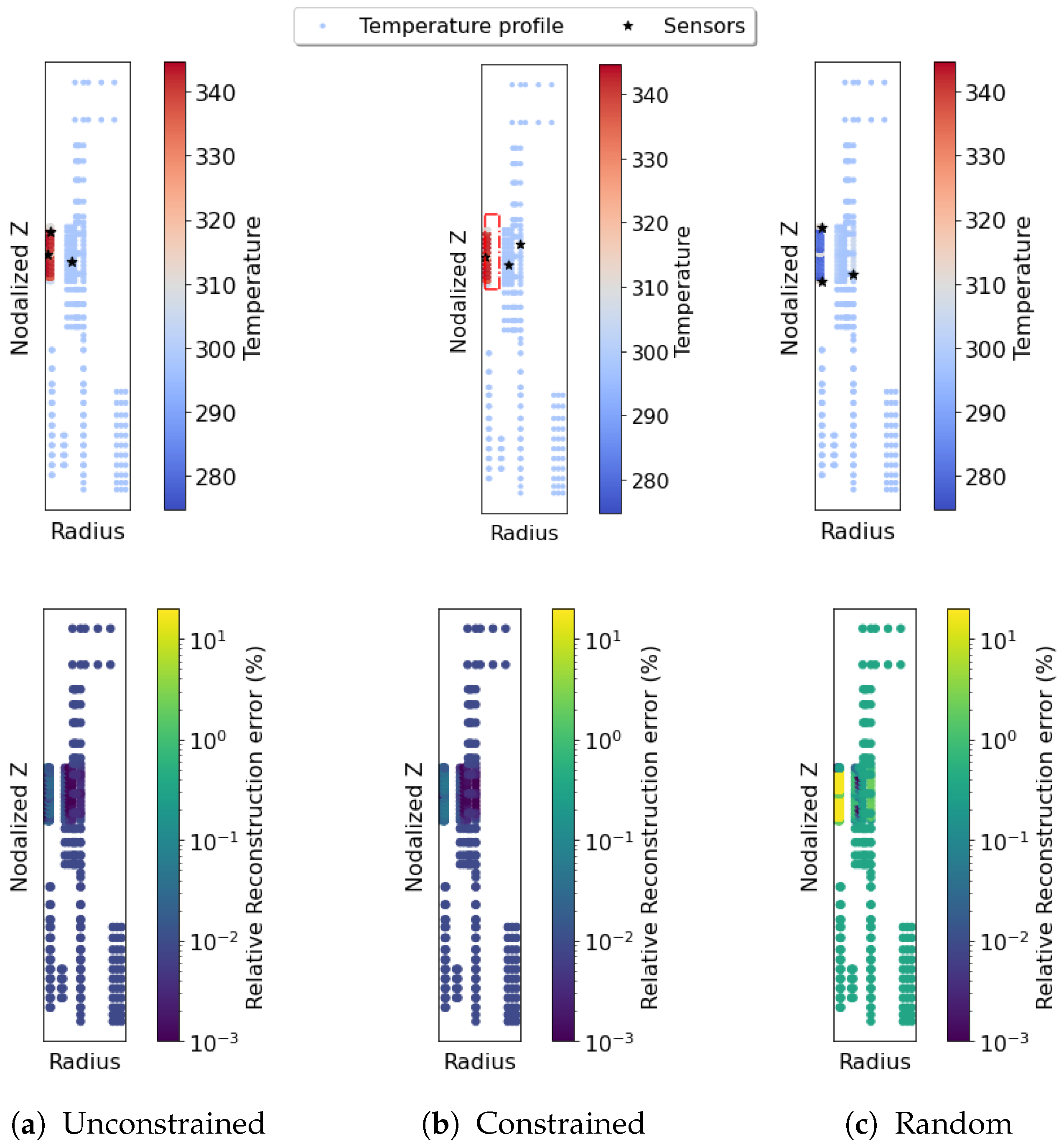
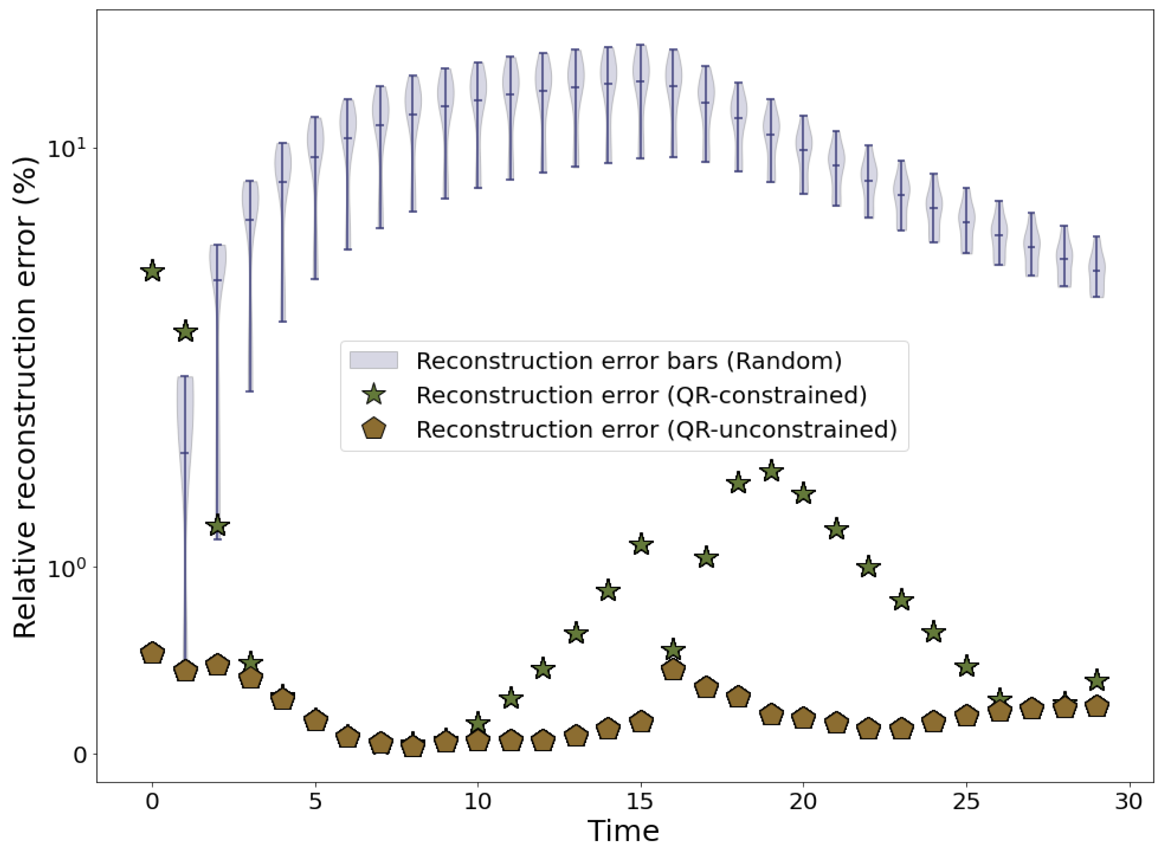
where $P_t=500$ W, $P_n=0$ W, and $t_1=15$ s. The power rises to 500 W within the first 15 s and remains off for the next 85 s. Heat flow through the capsule during this transient is simulated by the nodalization of the OPTI-TWIST geometry to capture temperature gradients in RELAP (described in Section 2.1.2). K- and N-type TCs are used for instrumentation of the rod (Figure 5), with their number restricted to $p=3$. The unconstrained QR method places two sensors near the heater, as seen in Figure 24a, capturing richer dynamics close to the heat source and resulting in a maximum relative reconstruction error of $ϵ=$ 0.06%. However, spatial constraints limit TC placement to just one sensor in this region (Figure 24b), resulting in a comparable $ϵ=$ 0.15%. POD modes, averaging over the time domain for time-dependent data, capture maximum variance in the temperature profile. When the heater power is at 500 W, the temperature variation is around 60 °C, whereas it becomes negligible when the power is off. Randomly placed sensors, with two located near the heater, fail to capture this temperature variation, resulting in high errors ($ϵ$ = 30%) reconstructing the OPTI-TWIST temperature profile (Figure 24c). Errors are calculated for the temperature profile at 8 s (mid-way through the transient). For the first two time-steps, the reconstruction error for an ensemble of twenty combinations of three randomly placed sensors (pink error bars) is comparable to QR placements (Figure 25). Subsequently, as the algorithm captures temperature variation, QR sensors result in significantly lower reconstruction errors ($ϵ=$ 0.2%) as compared to randomly placed sensors ($ϵ=$ 75%) over the transient domain. As the transient subsides, the error for both QR-optimized and random sensors briefly increases as the capsule cools down and temperature differences diminish. While POD modes capture maximum temperature variance during the transient, further analyses using DMD, DMDc, and time-delayed embedding are needed to accurately model the transient’s time-dependent nature.

The uncertainty in state reconstruction due to noisy measurements is calculated using Equation (7). Adding Gaussian i.i.d noise $\eta \sim \mathcal{N}(0,0.01)$ results in higher uncertainty (0.825 °K) around the heater when sensors are constrained away from the heat source (Figure 26b) as compared to unconstrained heater-adjacent sensors (0.009 °K) (Figure 26a). For three randomly selected sensors near the heater, the uncertainty in reconstruction is high (${10}^3$ °K) for regions adjacent to the heat source (Figure 26c). Optimizing sensor locations to capture underlying dynamics reduces reconstruction errors and uncertainty from TC readings in the presence of noise. This optimization enables the establishment of digital twins (DTs) for reliability and safety analysis of power transients and surges in nuclear fuel rods.

4. Discussion and Conclusions

This research heralds a transformative approach in managing the lifecycle of complex systems, spanning from initial design to eventual retirement. Traditionally, the lifecycle has been characterized by sequential phases: design, prototype construction, prototype testing, full-scale unit construction, full-scale experimentation, model building, launch, and finally, retirement. This study proposes an innovative reordering by advancing the modeling stage to immediately follow the initial design phase. This adjustment leverages digital models to inform and refine prototype development and identifies optimal instrumentation placements for experimental validation.

Crucially, this methodology advocates for a concurrent virtual timeline, where artificial intelligence models support design, prototyping, and experimental design, including the strategic selection of sensors and instruments (S&Is). This digital-first mindset is poised to be a cornerstone of the fourth industrial revolution, dramatically reducing the costs associated with iterative processes.

Moreover, the strategic placement of sensors, coupled with the use of reconstruction reduced-order models (ROMs), facilitates the continuous validation of digital twins. This enhances real-time monitoring capabilities, enabling predictions of potential anomalies, off-normal conditions, and even subtle discrepancies at a pace surpassing real time. Consequently, this allows for the adjustment of physics-trained digital models [53] without the need for frequent retraining whenever unexplained discrepancies arise from sensor data. Instead, smaller, specialized models (such as neural networks) are developed to specifically address these discrepancies (i.e., discrepancy modeling [54,55]), thus maintaining operational continuity of the digital twins while delving deeper into the root causes of the observed deviations.

If a discrepancy is traced back to physical causes such as leakage or degradation, the digital twin system should recommend appropriate actions, such as scheduling maintenance or replacing components. Conversely, if the root cause points to the digital model and not the physical asset, this indicates potential oversights in the modeling process, necessitating a reconsideration of the model or calibration to incorporate missing physical dynamics.

This enhances all safety protocol and significantly elevates the operational standards of nuclear power plants by not only anticipating known accident scenarios but also by detecting and addressing anomalies that could detrimentally impact performance and efficiency. Additionally, the sensor placement algorithms introduced here enable full-field reconstructions, providing “virtual sensors” at critical yet physically inaccessible locations within harsh environments. These algorithms also aid in distinguishing physical patterns from instrumentation biases, and should be utilized to learn drifting patterns of specific sensors under specific conditions, thereby lending unprecedented rigor and reliability to power plant operations, enhancing diagnostics and prognostics, and ultimately raising efficiency levels during plant operation.

This work leverages computational models of NPP subsystems, including steam generators, fuel capsules, and fuel irradiation experiments, to provide optimal sensor locations subject to inherent spatial limitations. The developed data-driven approach applied to preliminary 1D simulations of the steam generator establish sensor layouts that capture multiple fields of interest with high accuracy. They also provide interpretable models to study boiling regimes in steam generators. Further, TC locations that are identified by the algorithm for the 3D CFD model of the steam generator are able to capture temperature variations as the mass flow rate of the primary coolant changes. Flow distribution within the shell and tube can be accurately reconstructed with just one instrumented tube and the rest of the sensors constrained to the shell. In TRISO fuel irradiation experiments, sensors constrained to lie in the graphite holder outside the fuel accurately reconstruct the temperature within the fuel with low noise-induced uncertainty. In the event of sudden increases in power during accident scenario testing in fuel rods, sensor layouts capture temperature variations across the transient while constraining sensors to lie outside the heater-adjacent region. It is desirable to place the fewest number of sensors in locations that have extreme conditions (TRISO fuel) or where sensors would obstruct the development of nominal flow (SG tubes). We show that accurate reconstruction can be achieved with as few as three intrusive sensors. In conclusion, constrained sensor locations minimize reconstruction errors and provide statistical bounds for noise-induced uncertainties for high-dimensional nuclear applications that can be further used for safety analysis, licensing, accident scenario testing, and reliability analysis of the NPP.

Constrained sensor-based reconstruction of responses of interest from different subsystems, including temperature measurements from the reactor core, heat flux, pressure, and velocity in the steam generator, can enable the formation of individual DTs.Networks of individual DTs can form aggregates that inform control decisions, detect anomalies, and lead to enhanced safety of the NPP. Constraints for these test cases arise from experimental requirements, space availability, ease of maintenance, and in ensuring structural integrity. Constraints on sensor locations are selected by prioritizing end users and best practices to capture dynamics of the flow. Established digital twinning framework leverages computational models for the non-destructive testing of failure modes. Through CFD, FEM, and Python models, the effectiveness of adaptive sensor placement and accuracy of the reconstructed responses of interest have been demonstrated. Moreover, the scalability and broad applicability of the algorithms on a variety of applications and constraints have been showcased.

Nevertheless, to form DT aggregates, it is important to infer another field of interest through a sensor-based reconstruction of a particular response, for example, by inferring heat flux from temperature or primary-side pressure from available measurements of secondary-side pressure in the steam generator. When off-normal working conditions arise due to power transients or loss of power in one of the subsystems, accurate measurements lead to early detection of anomalies and enhance safety and security of the NPP. Tube breaks in the steam generator play a crucial role for safe operating conditions. Optimizing sensor locations for tube breakage prediction and classification is a challenge for DTs. Such early-stage anomaly and accident detection would enable further improvement of the presented model with added features for interpretability of advanced DTs for nuclear applications.

Although, an accurate and real-time reconstruction of flow fields are test-case-specific, as presented in this study, understanding the potential challenges in the verification and validation efforts would lead to the development of useful computational models. For nuclear systems, DTs and data analytics models would eventually require features like explainability and trustworthiness, which will be the future research direction of this study.

References

1. International Atomic Energy Agency. Core Knowledge on Instrumentation and Control Systems in Nuclear Power Plants; IAEA Nuclear Energy Series; No. NP-T-3.12, Technical Report; International Atomic Energy Agency: Vienna, Austria, 2011. [Google Scholar]
2. Fernandez, A.F.; Gusarov, A.I.; Brichard, B.t.; Bodart, S.; Lammens, K.; Berghmans, F.; Decreton, M.; Megret, P.; Blondel, M.; Delchambre, A. Temperature monitoring of nuclear reactor cores with multiplexed fiber Bragg grating sensors. Opt. Eng. 2002, 41, 1246–1254. [Google Scholar]
3. Messai, A.; Mellit, A.; Abdellani, I.; Pavan, A.M. On-line fault detection of a fuel rod temperature measurement sensor in a nuclear reactor core using ANNs. Prog. Nucl. Energy 2015, 79, 8–21. [Google Scholar] [CrossRef]
4. Hashemian, H.M. On-line monitoring applications in nuclear power plants. Prog. Nucl. Energy 2011, 53, 167–181. [Google Scholar] [CrossRef]
5. Upadhyaya, B.; Perillo, S.; Xu, X.; Li, F. Advanced control design, optimal sensor placement, and technology demonstration for small and medium nuclear power reactors. In Proceedings of the International Conference on Nuclear Engineering, Brussels, Belgium, 12–16 July 2009; Volume 43550, pp. 763–773. [Google Scholar]
6. Argaud, J.P.; Bouriquet, B.; De Caso, F.; Gong, H.; Maday, Y.; Mula, O. Sensor placement in nuclear reactors based on the generalized empirical interpolation method. J. Comput. Phys. 2018, 363, 354–370. [Google Scholar] [CrossRef]
7. Li, F.; Upadhyaya, B.R. Design of sensor placement for an integral pressurized water reactor using fault diagnostic observability and reliability criteria. Nucl. Technol. 2011, 173, 17–25. [Google Scholar] [CrossRef]
8. Upadhyaya, B.R.; Li, F. Optimal sensor placement strategy for anomaly detection and isolation. In Proceedings of the 2011 Future of Instrumentation International Workshop (FIIW) Proceedings, Oak Ridge, TN, USA, 7–8 November 2011; pp. 95–98. [Google Scholar]
9. Khalil Ur, R.; Shin, J.; Zubair, M.; Heo, G.; Son, H. Sensitivity study on availability of I&C components using bayesian network. Sci. Technol. Nucl. Install. 2013, 2013, 656548. [Google Scholar]
10. Li, W.; Peng, M.; Wang, Q. Improved PCA method for sensor fault detection and isolation in a nuclear power plant. Nucl. Eng. Technol. 2019, 51, 146–154. [Google Scholar] [CrossRef]
11. Oh, D.Y.; No, H.C. Determination of the minimal number and optimal sensor location in a nuclear system with fixed incore detectors. Nucl. Eng. Des. 1994, 152, 197–212. [Google Scholar] [CrossRef]
12. Hashemian, H.; Bean, W.C. Sensors for next-generation nuclear plants: Fiber-optic and wireless. Nucl. Sci. Eng. 2011, 169, 262–278. [Google Scholar] [CrossRef]
13. He, R.; Chen, G.; Dong, C.; Sun, S.; Shen, X. Data-driven digital twin technology for optimized control in process systems. ISA Trans. 2019, 95, 221–234. [Google Scholar] [CrossRef]
14. Willcox, K. Unsteady flow sensing and estimation via the gappy proper orthogonal decomposition. Comput. Fluids 2006, 35, 208–226. [Google Scholar] [CrossRef]
15. Yildirim, B.; Chryssostomidis, C.; Karniadakis, G. Efficient sensor placement for ocean measurements using low-dimensional concepts. Ocean Model. 2009, 27, 160–173. [Google Scholar] [CrossRef]
16. Manohar, K.; Brunton, B.W.; Kutz, J.N.; Brunton, S.L. Data-driven sparse sensor placement for reconstruction: Demonstrating the benefits of exploiting known patterns. IEEE Control Syst. Mag. 2018, 38, 63–86. [Google Scholar]
17. Brunton, B.W.; Brunton, S.L.; Proctor, J.L.; Kutz, J.N. Sparse sensor placement optimization for classification. SIAM J. Appl. Math. 2016, 76, 2099–2122. [Google Scholar] [CrossRef]
18. Mohren, T.L.; Daniel, T.L.; Brunton, S.L.; Brunton, B.W. Neural-inspired sensors enable sparse, efficient classification of spatiotemporal data. Proc. Natl. Acad. Sci. USA 2018, 115, 10564–10569. [Google Scholar] [CrossRef]
19. Bigoni, C.; Zhang, Z.; Hesthaven, J.S. Systematic sensor placement for structural anomaly detection in the absence of damaged states. Comput. Methods Appl. Mech. Eng. 2020, 371, 113315. [Google Scholar] [CrossRef]
20. Jamei, M.; Scaglione, A.; Roberts, C.; Stewart, E.; Peisert, S.; McParland, C.; McEachern, A. Anomaly Detection Using Optimally Placed μPMU Sensors in Distribution Grids. IEEE Trans. Power Syst. 2017, 33, 3611–3623. [Google Scholar] [CrossRef]
21. Krause, A.; Singh, A.; Guestrin, C. Near-optimal sensor placements in Gaussian processes: Theory, efficient algorithms and empirical studies. J. Mach. Learn. Res. 2008, 9, 235–284. [Google Scholar]
22. Pei, X.Y.; Yi, T.H.; Qu, C.X.; Li, H.N. Conditional information entropy based sensor placement method considering separated model error and measurement noise. J. Sound Vib. 2019, 449, 389–404. [Google Scholar] [CrossRef]
23. Paninski, L. Asymptotic theory of information-theoretic experimental design. Neural Comput. 2005, 17, 1480–1507. [Google Scholar] [CrossRef]
24. Wang, S.; Lai, X.; He, X.; Li, K.; Lv, L.; Song, X. Optimal sensor placement for digital twin based on mutual information and correlation with multi-fidelity data. Eng. Comput. 2024, 40, 1289–1308. [Google Scholar] [CrossRef]
25. Caselton, W.F.; Zidek, J.V. Optimal monitoring network designs. Stat. Probab. Lett. 1984, 2, 223–227. [Google Scholar] [CrossRef]
26. Lin, X.; Chowdhury, A.; Wang, X.; Terejanu, G. Approximate computational approaches for Bayesian sensor placement in high dimensions. Inf. Fusion 2019, 46, 193–205. [Google Scholar] [CrossRef]
27. Donoho, D.L. Compressed sensing. IEEE Trans. Inf. Theory 2006, 52, 1289–1306. [Google Scholar] [CrossRef]
28. Candes, E.J.; Tao, T. Near-optimal signal recovery from random projections: Universal encoding strategies? IEEE Trans. Inf. Theory 2006, 52, 5406–5425. [Google Scholar] [CrossRef]
29. Akbarzadeh, V.; Gagné, C.; Parizeau, M.; Mostafavi, M.A. Black-box optimization of sensor placement with elevation maps and probabilistic sensing models. In Proceedings of the 2011 IEEE International Symposium on Robotic and Sensors Environments (ROSE), Montreal, QC, Canada, 17–18 September 2011; pp. 89–94. [Google Scholar]
30. Summers, T.H.; Cortesi, F.L.; Lygeros, J. On submodularity and controllability in complex dynamical networks. IEEE Trans. Control Netw. Syst. 2015, 3, 91–101. [Google Scholar] [CrossRef]
31. Joshi, S.; Boyd, S. Sensor selection via convex optimization. IEEE Trans. Signal Process. 2008, 57, 451–462. [Google Scholar] [CrossRef]
32. Chepuri, S.P.; Leus, G. Continuous sensor placement. IEEE Signal Process. Lett. 2014, 22, 544–548. [Google Scholar] [CrossRef]
33. Liu, S.; Chepuri, S.P.; Fardad, M.; Maşazade, E.; Leus, G.; Varshney, P.K. Sensor selection for estimation with correlated measurement noise. IEEE Trans. Signal Process. 2016, 64, 3509–3522. [Google Scholar] [CrossRef]
34. Chaturantabut, S.; Sorensen, D.C. Nonlinear model reduction via discrete empirical interpolation. SIAM J. Sci. Comput. 2010, 32, 2737–2764. [Google Scholar] [CrossRef]
35. Drmac, Z.; Gugercin, S. A new selection operator for the discrete empirical interpolation method—Improved a priori error bound and extensions. SIAM J. Sci. Comput. 2016, 38, A631–A648. [Google Scholar] [CrossRef]
36. Manohar, K.; Kutz, J.N.; Brunton, S.L. Optimal sensor and actuator selection using balanced model reduction. IEEE Trans. Autom. Control 2021, 67, 2108–2115. [Google Scholar] [CrossRef]
37. Clark, E.; Kutz, J.N.; Brunton, S.L. Sensor selection with cost constraints for dynamically relevant bases. IEEE Sens. J. 2020, 20, 11674–11687. [Google Scholar] [CrossRef]
38. Clark, E.; Askham, T.; Brunton, S.L.; Kutz, J.N. Greedy sensor placement with cost constraints. IEEE Sens. J. 2018, 19, 2642–2656. [Google Scholar] [CrossRef]
39. Clark, E.; Brunton, S.L.; Kutz, J.N. Multi-fidelity sensor selection: Greedy algorithms to place cheap and expensive sensors with cost constraints. IEEE Sens. J. 2020, 21, 600–611. [Google Scholar] [CrossRef]
40. Manohar, K.; Kaiser, E.; Brunton, S.L.; Kutz, J.N. Optimized sampling for multiscale dynamics. Multiscale Model. Simul. 2019, 17, 117–136. [Google Scholar] [CrossRef]
41. Klishin, A.A.; Kutz, J.N.; Manohar, K. Data-Induced Interactions of Sparse Sensors. arXiv 2023, arXiv:2307.11838. [Google Scholar]
42. Karnik, N.; Abdo, M.G.; Estrada-Perez, C.E.; Yoo, J.S.; Cogliati, J.J.; Skifton, R.S.; Calderoni, P.; Brunton, S.L.; Manohar, K. Constrained optimization of sensor placement for nuclear digital twins. IEEE Sens. J. 2024, 24, 15501–15516. [Google Scholar] [CrossRef]
43. RELAP5-3D© Code Development Team. RELAP5-3D© Code Manual Volume II: User’s Guide and Input Requirements; Technical Report; Idaho National Lab. (INL): Idaho Falls, ID, USA, 2015. [Google Scholar]
44. Palmer, A.; Skifton, R.; Scervini, M.; Haggard, D.; Swank, W. Performance of custom-made very high temperature thermocouples in the advanced gas reactor experiment AGR-5/6/7 during irradiation in the advanced test reactor. EPJ Web Conf. 2020, 225, 04010. [Google Scholar] [CrossRef]
45. Sporian Microsystems, Inc. ThermalFlow 700; Sporian Microsystems Inc.: Lafayette, CO, USA, 2024. [Google Scholar]
46. Everson, R.; Sirovich, L. Karhunen–Loeve procedure for gappy data. JOSA A 1995, 12, 1657–1664. [Google Scholar] [CrossRef]
47. Fisher, R.A. Statistical Methods for Research Workers. In Breakthroughs in Statistics: Methodology and Distribution; Springer: New York, NY, USA, 1970; pp. 66–70. [Google Scholar]
48. Businger, P.; Golub, G.H. Linear least squares solutions by Householder transformations. Numer. Math. 1965, 7, 269–276. [Google Scholar] [CrossRef]
49. Gu, M.; Eisenstat, S.C. Efficient algorithms for computing a strong rank-revealing QR factorization. SIAM J. Sci. Comput. 1996, 17, 848–869. [Google Scholar] [CrossRef]
50. Kochunas, B.; Huan, X. Digital twin concepts with uncertainty for nuclear power applications. Energies 2021, 14, 4235. [Google Scholar] [CrossRef]
51. Wilkins, S.C. Low Cross-Section Mo-Nb Thermocouples for Nuclear Application: The State-of-the-Art; Technical report; EG and G Idaho, Inc.: Idaho Falls, ID, USA, 1988. [Google Scholar]
52. Skifton, R. High-temperature irradiation-resistant thermocouple instability model for in-pile reactor use. Front. Energy Res. 2023, 11, 1099584. [Google Scholar] [CrossRef]
53. Gong, H.; Cheng, S.; Chen, Z.; Li, Q. Data-enabled physics-informed machine learning for reduced-order modeling digital twin: Application to nuclear reactor physics. Nucl. Sci. Eng. 2022, 196, 668–693. [Google Scholar] [CrossRef]
54. Kaheman, K.; Kaiser, E.; Strom, B.; Kutz, J.N.; Brunton, S.L. Learning discrepancy models from experimental data. arXiv 2019, arXiv:1909.08574. [Google Scholar]
55. Ebers, M.R.; Steele, K.M.; Kutz, J.N. Discrepancy modeling framework: Learning missing physics, modeling systematic residuals, and disambiguating between deterministic and random effects. arXiv 2022, arXiv:2203.05164. [Google Scholar] [CrossRef]
56. de Silva, B.M.; Manohar, K.; Clark, E.; Brunton, B.W.; Kutz, J.N.; Brunton, S.L. PySensors: A Python package for sparse sensor placement. J. Open Source Softw. 2021, 6, 2828. [Google Scholar] [CrossRef]
57. Rabiti, C.; Alfonsi, A.; Mandelli, D.; Cogliati, J.J.; Wang, C.; Talbot, P.W.; Malijovec, D.P.; Kinoshita, R.A.; Abdo, M.G.; Sen, S.; et al. RAVEN User Manual; Technical report; Idaho National Lab. (INL): Idaho Falls, ID, USA, 2021. [Google Scholar]
Figure 1. Optimized sensor placement in individual subsystems of nuclear power plants allows for real-time two-way communication between the physical asset and its digital twin. It further empowers digitally enabled decision-making, control strategies, predictive maintenance, and risk assessment to form a network of DTs called aggregates.
Energies 17 03355 g001
Figure 2. Irradiation of TRISO fuel experiment in the advanced test reactor.
Energies 17 03355 g002
Figure 3. OPTI-TWIST RELAP nodalization for simulating thermal-hydraulic behavior of test fuel rods.
Energies 17 03355 g003
Figure 4. HTIR-TCs can withstand temperatures up to 1600 °C and are used in graphite holders for irradiation of TRISO fuel experiments. They exhibit high sensitivity at 900 °C, but due to higher experimental temperatures, precise placement is crucial for accurate measurements [44].
Energies 17 03355 g004
Figure 5. A series of K-type thermocouples are arranged at various heights for temperature monitoring in the OPTI-TWIST experiment.
Energies 17 03355 g005
Figure 6. One-dimensional model of a steam generator, which empirically simulates boiling phenomena occurring in the SG at different heights.
Energies 17 03355 g006
Figure 7. Three-dimensional CAD of the primary side which models 1/4th of the steam generator.
Energies 17 03355 g007
Figure 8. Discretization of SG geometry using a polyhedral mesh and boundary conditions generated in Star-CCM+ 2210 (17.06.008-R8).
Energies 17 03355 g008
Figure 9. Sporian ThermaFlowTM 700 velocity sensor and technical specifications [45].
Energies 17 03355 g009
Figure 10. Pressure taps and fiber-optic-based pressure sensors can be placed anywhere in the secondary tubes to provide localized pressure measurements.
Energies 17 03355 g010
Figure 11. Square sensors mounted to the outer and/or inner surface of the wall can be used for heat flux measurements.
Energies 17 03355 g011
Figure 12. The secondary-side temperature, flux, and pressure can be accurately reconstructed with minimal reconstruction uncertainty using only 3 QR-constrained sensors. The sampling rate is p / n = 0.27 % .
Energies 17 03355 g012
Figure 13. The leading three POD modes of secondary-side temperature accurately approximate temperature fields with 99% of the energy content. The first mode captures the overall temperature profile, and the second and third modes capture heat flux variations along the normalized z-coordinates in the steam generator.
Energies 17 03355 g013
Figure 14. Temperature and velocity sensor locations for unconstrained, constrained, and randomly placed sensors. Unconstrained QR places 2 temperature and 3 velocity sensors in the tubes (z < 1.828 m) highlighted by the red boxes. Physically, just one of the tubes is instrumented. Constrained QR restricts just one temperature and one velocity sensor within tubes (green boxes).
Energies 17 03355 g014
Figure 15. QR-optimized sensors reconstruct the temperature field with high accuracy (a). Constraining a single sensor to lie within one of the steam generator tubes results in only a minimal increase in error and noise-induced uncertainty for temperature reconstruction (b), compared to the high error of randomly placed sensor reconstructions (c). (Top) Sensor-based reconstructions. (Middle) Relative reconstruction error. (Bottom) Noise-induced uncertainty heatmaps (log scale).
Energies 17 03355 g015
Figure 16. QR-optimized sensors capture temperature variance within the SG, leading to higher reconstruction accuracy across all mass flow rates compared to random sensor placement. Optimized sensors achieve low reconstruction errors ( ϵ 0.34 % ), and random placements result in larger errors ( ϵ 2 % ). Plot is shown on a symbolic log scale to highlight differences in reconstruction errors.
Energies 17 03355 g016
Figure 17. QR-optimized sensors (both unconstrained and constrained) detect the underlying dynamics of coolant flow within the SG and reconstruct the velocity field with high accuracy and low noise-induced uncertainties (a,b). By contrast, random sensors are unable to reconstruct the field, resulting in high errors and uncertainty (c). (Top) Sensor-based reconstructions. (Middle) Relative reconstruction error. (Bottom) Noise-induced uncertainty heatmaps (log scale).
Energies 17 03355 g017
Figure 18. QR-optimized sensors capture flow of the coolant through the riser as it make a 180° turn through the shell, leading to higher reconstruction accuracy across all mass flow rates compared to random sensor placement. Optimized sensors achieve low reconstruction errors ( ϵ 0.05 m/s), while random placements result in much larger errors ( ϵ 25 m/s). Plot is shown on a symbolic log scale to highlight differences in reconstruction errors.
Energies 17 03355 g018
Figure 19. Temperature profile of the fuel capsule at the end-of-cycle stage. The temperature in the fuel reaches 1250 °C (b), compared to around 1000 °C in the graphite holder (a). Accurate reconstruction of the temperature profile within the fuel through TCs is crucial due to the richer dynamics inside the TRISO fuel (c).
Energies 17 03355 g019
Figure 20. The unconstrained sensor locations (a) are infeasible since one of the thermocouples is placed in the fuel. The developed algorithm constrains the TCs to lie within potential structural holes (red circles) (b), selecting drill locations where the drill depth is given by the Z coordinate, and the random sensor layout is shown in (c). Green stars reflect sensor locations.
Energies 17 03355 g020
Figure 21. QR-optimized sensors reconstruct temperature profiles within both the TRISO fuel (3rd column, 4th row (a,b)) and the graphite holder (1st column, 2nd row (a,b)) when compared to random sensor locations (c). (1st row) Sensor-based reconstructions. (2nd row) Relative reconstruction error. (3rd row) Fuel reconstruction through sensors. (4th row) Fuel relative reconstruction error.
Energies 17 03355 g021
Figure 22. QR-optimized sensors are the most accurate in capturing the neutron and gamma heating dynamics at both beginning-of-cycle and end-of-cycle stages. Optimized sensors reconstruct temperature fields with low errors ( ϵ 1 % ), whereas random placements result in significantly larger errors ( ϵ 30 % ). Plot is shown on a symbolic log scale to highlight differences in reconstruction errors.
Energies 17 03355 g022
Figure 23. Optimized sensors result in lower estimation uncertainty in state reconstruction within the fuel when sensor measurements are corrupted by noise (a,b) compared to random placement (c). These estimation errors propagate through the digital twin and affect downstream control decisions. Plots are shown on a log scale to highlight regions of higher uncertainty.
Energies 17 03355 g023
Figure 24. Richer dynamics close to the heat source result in the selection of unconstrained sensors near the heater (a-top), achieving negligible reconstruction error ϵ = 0.06 % (a-bottom). However, these locations are unfeasible as the heater cannot accommodate multiple sensors. Constraining sensors to lie outside the heater region (b-top) produces a layout with comparable reconstruction errors ϵ = 1 % (b-bottom). Random sensor placement leads to inaccurate reconstructions (c-top) with high reconstruction errors ϵ 10 1 % (c-bottom).
Energies 17 03355 g024
Figure 25. Constrained QR-optimized sensors initially fail to capture temperature variation at t = 0 due to the transient but achieve lower error as the transient progresses ( ϵ 0.5 % ). Once the transient ends at t = 15, constrained QR reconstruction error briefly rises before capturing the cooling down of the capsule. Reconstruction error for ensembles of randomly selected sesnors increases and then stays the same with time ( ϵ 75 % ), while unconstrained QR sensors placed in heater-adjacent locations result in the lowest error through the entire transient. Plot is shown on a symbolic log scale to highlight differences in reconstruction errors.
Energies 17 03355 g025
Figure 26. When sensors are constrained to lie outside the heater region (b), the uncertainty in the heater region increases slightly by 0.95 °K, and for randomly placed sensors, it can increase up to 1000 °K.
Energies 17 03355 g026
Disclaimer/Publisher’s Note: The statements, opinions and data contained in all publications are solely those of the individual author(s) and contributor(s) and not of MDPI and/or the editor(s). MDPI and/or the editor(s) disclaim responsibility for any injury to people or property resulting from any ideas, methods, instructions or products referred to in the content.