Abstract
Today, the analysis and synthesis methods of electro-pneumatic systems with position control actuated by pneumatic artificial muscles (PAMs) are quite well known. In these methods, pneumatic artificial muscle is considered as an object with lumped parameters. However, the PAM is an object with distributed parameters, where the pressure, density, and mass flow rate of gas are varied along the bladder length. Thus, in the case of certain design parameters of the pneumatic artificial muscle and certain frequencies of the supply pressure, resonant gas oscillations affected by the wave processes in the bladder may occur. Thereby, in the PWM-driven PAM-actuated system, certain operation frequencies of the control pneumatic valve can cause oscillations of gas in the bladder and in the connected pipeline. These processes could lead to vibrations of the executive device. To solve this practical problem, a distributed parameter model of the PAM that takes into account the pressure fluctuations in the bladder and in the pipeline was elaborated. Also, in this work, a new method in which the wave processes are described by ordinary differential equations instead of partial differential equations was proposed.
1. Introduction
In recent years, many researchers have devoted themselves to investigations on pneumatic systems based on pneumatic artificial muscles (PAMs). PAMs are used in industrial applications as parts of manipulators for lifting and lowering a load [1,2], parallel platforms [3], dexterous anthropomorphic robots [4,5,6], and rehabilitation and orthotic devices [7,8,9,10].
PAM-actuated systems are usually built on electro-pneumatic valves and include a complex control system that contains different sensors and controllers. In modern electro-pneumatic systems, there are two types of valves used to control the flow rate in the actuator, i.e., the proportional (servo) valves and solenoid on–off (fast-switching) valves. Proportional control valves allow obtaining high control precision and have linear output characteristics. However, they are expensive and have a slow response speed, complex structure, and difficult maintenance compared to on–off valves. Nowadays, digital on–off solenoid valves with high switching speeds are available [11,12,13] and can be used instead of servo valves. They are simple and less expensive, but their flow characteristics are nonlinear. To linearize the volume flow characteristics of fast-switching valves, PWM techniques are generally used. In a number of studies, the authors proposed different PWM techniques to control the position of pneumatic cylinders [11,13,14,15,16,17,18,19] and pneumatic artificial muscles [12,20,21,22,23,24]. Typically, a PWM algorithm is used in conjunction with other control approaches, such as in the works mentioned above. The parameters, types of models, and control methods of pneumatic systems are presented in Table 1.
Many studies have focused on the development of control systems for PAM-actuated devices with the required performance characteristics. To address this problem and obtain high positioning accuracy of the executive device, different mathematical models have been elaborated and introduced.
Pneumatic artificial muscles are complex objects for modeling and their dynamic characteristics crucially depend on their construction and physical properties. Therefore, design of a PAM-actuated system with accurate and reliable positioning is a difficult task. PAMs are characterized by nonlinearity of force characteristics, threshold pressure, and phenomena such as hysteresis [5,25,26]. Additionally, PAM modeling is complicated due to the different types of commercial [27,28,29,30] and noncommercial muscles [31,32,33,34] and the impossibility of developing a universal equation of static force. Nowadays, most of the studies are mainly focused on the investigation of the characteristics and properties of the braided PAMs, such as McKibben pneumatic artificial muscles and commercial PAMs, designed by FESTO Company. The models of static force of McKibben PAMs are proposed in [5,25,34,35,36,37,38,39,40] and cannot be applied to FESTO PAMs. Models describing the static force of FESTO PAMs are presented in [41,42,43,44,45,46,47,48,49,50,51].
All models of PAMs can be divided into the three following types: analytical or geometric models, empirical models, and phenomenological models [31]. Geometric models are based on the geometry and physical properties of the pneumatic artificial muscle, while empirical models are based on experimental data. Geometric and empirical models are more suitable for describing the static characteristics of PAMs, whereas phenomenological models are applied to describe the dynamic behavior [48,49,52,53,54,55,56]. In Table A1 in Appendix A, a brief chronology of PAM models is presented.

Table 1.
Parameters of the electro-pneumatic systems with the PWM algorithm.
Table 1.
Parameters of the electro-pneumatic systems with the PWM algorithm.
| Authors, Year | Type of Model | Additional Control Method | PWM Frequency, Hz | PAM Characteristics |
|---|---|---|---|---|
| Ville T. Jouppila et al., 2014 [21] | geometric [42] | SMC | 100 | diameter: 30 mm length: 100 mm |
| Xie S. et al., 2016 [12] | empirical [47] | PID | 100–180 | diameter: 20 mm length: 500 mm |
| Pipan M., and Harakovic N. 2018 [22] | no data | PID | 250 | diameter: 20 mm length: 200 mm |
| Rimar M. et al., 2019 [23] | geometric [25] | – | 50 | diameter: 40 mm length: 1000 mm |
The main conclusions of the above review are as follows:
- The models mentioned above consider the pneumatic artificial muscle as an object with lumped parameters.
- As can be seen from Table 1, the impact of the design parameters of PAMs and PWM frequency of the control valve have not been studied in previous works. Also, in these works, the geometric and empirical mathematical models of PAMs are applied.
However, in this paper, a PAM is considered as an object with distributed parameters, i.e., the pressure, density, and viscosity of gas would be varied along the length of the bladder. Therefore, in the bladder of the PAM, resonant gas oscillations caused by the wave processes are possible. The resonant gas oscillations occur due to certain PAM parameters and certain frequencies of the supply pressure. This must be taken into account when designing a PAM-actuated system with position control based on a PWM algorithm. These gas oscillations can result in undesirable vibrations of the output link at the positioning point.
When designing an industrial pneumatic circuit, typically, the components are arranged in such a way as to reduce the length of the pipeline to provide minimum response of the control system. However, the elements can have large distances between each other. In this case, it is necessary to take into account the wave processes in the pipelines.
The goals of this this study are:
- to develop a distributed parameter mathematical model of the PAM with the connected pipeline;
- to carry out the numerical investigations of pressure change in the end of the bladder;
- to explore the impact of the parameters of the pneumatic artificial muscle and pneumatic circuit on the wave processes;
- to create a methodology for finding out undesirable PWM frequencies of the control pressure.
The main contribution in this study was made by Donskoy A.S., who is the author of the method for describing wave processes in pipelines using ordinary partial equations [57]. The previous studies dedicated to the development and experimental validation of the PAM model were conducted by Donskoy et al. [41,50].
This paper is organized as follows. Section 2 presents the description of the PAM-actuated system with a PWM control signal. It contains the brief review of the mathematical models of pneumatic pipelines with distributed parameters. Also, in Section 2, the distributed parameter model with ODEs of a PAM with the connected supply pipeline is synthesized. The approach for calculation of the pressure change with ODEs is proposed and substantiated. The results and discussion of the numerical investigations are given in Section 3. The summary of this study presented drawn in Section 4.
2. Methods
2.1. Object of the Study
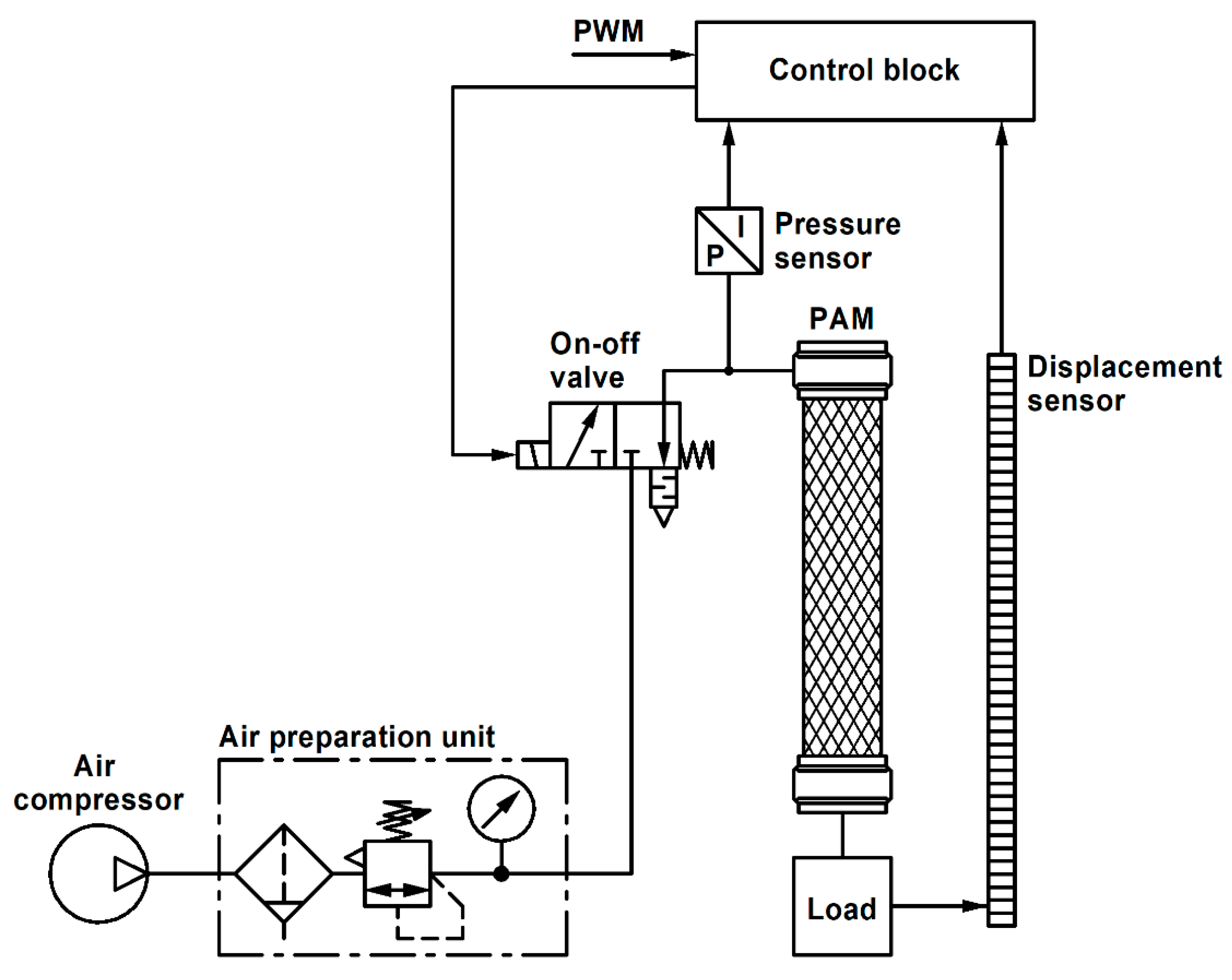
Figure 1 shows a PAM-actuated system with a PWM signal control. The PAM-actuated device consists of the PAM that connects with a load, and on–off valve that controls the airflow in the bladder. The control system consists of control block, pressure sensor, and displacement sensor. The control block transmits a PWM signal to the valve solenoid, converts the output analog signal to digital from the displacement sensor, and compares it with the desired position of a load.
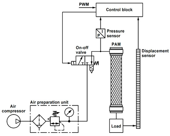
Figure 1.
A PAM-actuated system with a PWM signal control.
The air compressor connects with the air preparation unit and delivers a volume of air in the system. The air preparation unit consists of a filter, a relief valve, and a manometer that controls the degree of contamination of the filter. When the on–off valve is shut down, the PAM is connected with the external environment and the pressure in the bladder is equal to atmospheric pressure. The valve opening area and thereby the flow rate of compressed air change according to a PWM control signal. When a PWM signal from the control block excitates the solenoid, the on–off valve opens and delivers the pressurized air into the PAM, which results in contraction of the bladder. The PAM produces force and lifts the load. The pressure sensor and the displacement sensor connect with the control block and measure the current pressure in the bladder and the current coordinate of the load accordingly. Then, the analog signals are sent to the control block with the analog–digital converter. During the control of the output link position, the duty cycle of the PWM control signal is decreased proportionally to the error of the desired coordinate. When a load reaches the desired position, the PWM control signal is set to zero.
2.2. Proposed Approach
Existing mathematical models of the wave processes in pneumatic lines are based on relationships between the following gas parameters: pressure, velocity, density, and viscosity. These relationships are usually described by the following equations: Navier–Stokes equations (continuity equation and momentum equation), the ideal gas law equation, and equation of empiric viscosity [58]; therefore, they are defined as a set of partial differential equations (PDEs) [58,59,60,61,62,63,64]. In [58,63,64], different numerical methods for the solution of PDEs are presented.
These approaches significantly complicate numerical investigation of the wave processes. Modelling of pneumatic pipelines with the application of PDEs is a complex task, especially when considering the dynamics of other system objects such as pumps, valves, and tanks. The different approximation methods of PDEs limit the use of such models. Additionally, since the gas dynamics equations roughly describe the physical phenomena, these models do not always give accurate simulation results.
In PWM control systems, the positioning regime is the most undesirable regime, since the occurrence of the resonant gas oscillations can happen at the desired coordinate with the highest probability. With this consideration, the following assumptions can be made:
- To estimate possibility of gas oscillation occurrence at the positioning point, it is necessary to obtain the pressure change characteristics at the end of the PAM instead of this distribution along the bladder length.
- At the positioning point, the amplitude of the output link oscillations is negligible compared to the PAM’s entire length. Therefore, the change in the bladder length can be neglected and we can consider a PAM as a pipeline.
Therefore, the task can be simplified and we can apply the methodology of calculation of the pressure change at the ends of a pipeline [57]. With this approach, the wave processes can be described by ordinary differential equations (ODEs), since at the positioning point, they would be equal to PDEs. In [57], a comparison of the results of modeling wave processes using PDEs and using ODEs, as well as a comparison with experimental data, is given. The solutions obtained using ODEs show good convergence results, both with solutions using the PDE and with experimental data. The proposed method allows us to obtain simulation results with accuracy up to 5% and is universal for all types of pneumatic lines. In addition, this method is confirmed by other independent researchers [65,66].
Nowadays, there are many types of PAMs, from those widespread in industry (FESTO fluidic muscle, Shadow Air Muscle, Rubbertuator) to noncommercial PAMs [31,32,33]. The elaborated model considers the PAM bladder as a pipeline and universal for all types of PAMs. After obtaining simulation results using this model, the calculations can be continued with the models mentioned above, which take into account physical properties and construction parameters of the chosen type of PAM.
2.3. Distributed Parameter Mathematical Model
The system of the pneumatic artificial muscle with the supply pipeline (system «Pipeline—PAM») is presented in Figure 2.
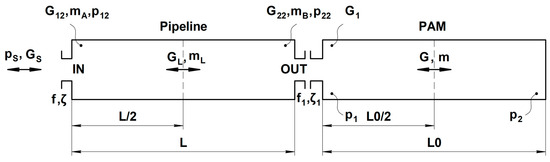
Figure 2.
System «Pipeline—PAM».
In order to elaborate the model of this system, the following processes are considered:
- The process of the gas mass acceleration leads to change in the flow rate inside the bladder and the pipeline.
- The process of the gas mass change due to the filling/emptying processes leads to change in the gas pressure, density, and mass flow rate.
- The process of the pressure change at the ends of the bladder and the pipeline is due to the wave processes.
The mathematical model of a PAM-actuated system, taking into account the wave processes, consists of the following equations:
- The equation of the gas motion in the pipeline.
- The equation of the gas motion in the bladder.
- The equations of the average mass flow rate and flow rates at the inlet and at the outlet of the pipeline.
- The equations of the average mass flow rate and the mass flow rate at the inlet of the PAM bladder.
According to the laws of gas dynamics, the pressure change in a given volume is determined by the difference between the incoming and outgoing flow rates and the value of this volume.
For our case, the following hypothesis was accepted. The pressure change at the inlet (the outlet) of the pneumatic line (the pipeline or the PAM bladder) is determined by the difference between the average mass flow rate and the mass flow rate at the inlet (the outlet) of the pneumatic line. The pressure changes according to the same law as the pressure in the pipeline, which volume is equal to half of the pipeline volume.
As can be seen from Figure 2, when compressed air with the pressure pS and the mass flow rate GS is delivered to the inlet of the pipeline, the pipeline is filled with the gas mass mL. According to the continuity equation, the mass flow rate GS at the inlet is equal to the mass flow rate G12 down the inlet of the pipeline. The movement of the gas mass mL inside the pipeline occurs under the influence of the pressure differential down the inlet p12 and at the outlet p22. The average mass flow rate GL and the flow rates on the ends of the pipeline would be different. Therefore, due these processes, the flow density changes at the ends of the pipeline and causes the pressure p22 to change. According to Figure 2, under the difference between the flow rates G12 and GL, the change in the pressure p12 occurs. The change in the pressure p22 occurs under the difference between GL and G22 at the outlet.
The time of the wave propagation [57,67] is
where L is the length of the pipeline, and c is the speed of sound.
t = L/c,
Consider the motion of the gas mass from the moment of delivering the supply pressure pS at the inlet of the pipeline.
The time t < L/c is the time from the pressure supply moment during the time of the wave propagation through the pipeline. For t < L/c, the pressure at the end of the pipeline is constant and is equal to initial value p220. At this time, the gas mass movement starts with some average speed due to the gas particle displacement at the inlet of the pipeline. At the same time, the speed of the gas at the outlet of the pipeline would be reduced, which leads to gas layer compression.
After time t = L/c, the pressure wave reaches the outlet of the pipeline. As a result, the pressure changes abruptly from p220 to some value p22. After that, the pressure changes permanently to the steady value.
The following assumptions are accepted:
- The gas mass movement is one-dimensional, i.e., the gas parameters are the functions of the z coordinate passing along the axis of the line.
- The considered processes are isothermal since the temperature change is negligible in most cases in pipelines of industrial systems.
- The length and the diameter of the pipeline and the PAM are constant (see the assumptions made in Section 2).
- The gas mass movement through the valves is quasi-static, i.e., the instantaneous value of gas consumption at the inlet in the transition processes is the same as in the steady-state flow at the same pressure drop.
- Dependence of the friction loss per the Reynolds number at the transitional process is the same as at the steady state [57]:
The air resistance coefficient λ is defined as [68]
In order to derive the equation of the gas movement in the pipeline, it is necessary to select volume with the mass mL. The pressure down the inlet p12 and the pressure at the end of the pipeline p22 impact the selected volume. Based on the above assumption, a one-dimensional gas flow is considered, so the pressure p12 and p22 would be distributed evenly over the pipeline cross-section. At the same time, the effect of the gas flow delivered to the inlet of the pipeline will be taken into account. With these considerations, the gas movement is described by the following system of equations [57]:
where mL is the current value of the gas mass in the pipeline, υ’ is the acceleration of the gas mass in the pipeline, fL = πDL/4 is the cross-section area of the pipeline, p12 is the pressure down the inlet of the pipeline, p22* is the current pressure at the end of the pipeline, p220 is the initial pressure at the end of the pipeline, p22 is the pressure characterizing the dynamics of gas layer compression at the end of the pipeline.
To obtain the solution of the system (4), the relationship between the pressures p12, p22, pFR and the average speed of the gas υ is defined below.
The current value of the gas mass mL in the pipeline is determined from the following equation:
where mA is the current value of the gas mass down the inlet of the pipeline, and mB is the current value of the gas mass at the outlet of the pipeline.
mL = mA + mB,
According to the continuity equation, the flow rate at the inlet is defined as
where G12 is the mass flow rate down the inlet of the pipeline.
m’A = GS = G12
The mass flow rate in the left half of the pipeline is obtained from the difference between the mass flow rate down the inlet of the pipeline and the average flow rate:
where GL is the average mass flow rate in the pipeline.
Considering the hypothesis given below, the pressure p12 changes according to the same law as the pressure in the pipeline, which volume is equal to half of the pipeline volume. The current value of the gas mass in the left half of the pipeline m12 is given by [68]
where VL is the current value of gas volume in the pipeline, VL = fLL.
The average gas density ρ according to the Clapeyron–Mendeleev equation is expressed as [68]
where TS is the gas temperature in the pipeline and the bladder, and R is the gas constant.
Substituting (9) in (8), the gas mass m12 is defined from the following equation:
Differentiating (10) and combining with (7), the pressure change for isothermal flow (TS = const) is expressed as
The average mass flow rate GL is given by
where υ is the average speed of the gas in the pipeline.
Merging (6) and (12) in (11), is obtained by
As mentioned above, the pressure at the end of the pipeline is constant during the time t of the wave propagation. When the wave reaches the end of the pipeline, the pressure abruptly changes its value. The magnitude of this jump and further change is determined by the degree of the gas compression at the end of the pipeline. The pressure change is determined by the amount of gas, which volume is equal to half of the pipeline volume.
The mass flow rate in the second half of the pipeline is defined as
where G22 is the mass flow rate at the outlet of the pipeline.
Similarly to Equation (10), the current value of the gas mass m22 in the second half of the pipeline is given by
Differentiating (15) and combining with (14), the pressure change for isothermal flow (TS = const) is expressed as
According to the continuity equation, the m’B is defined as
m’B = G22.
Through combining (12), (16), and (17), can be determined as
The average gas density ρ is given by
Then, Equation (2) for the friction loss in the pipeline, taking into account (19), can be written as
According to Figure 2, the equations for the mass flow rate at the inlet and at the outlet of the pipeline for the filling and emptying processes will look as follows [50,68,69]:
where f is the cross-section area of the pipeline inlet, f = πd/4, where d is the diameter of the pipeline inlet, ζ is the resistance coefficient of the pipeline inlet, pS is the pressure at the pipeline inlet, k is the polytropic coefficient, f1 is the cross-section area of the inlet of the PAM, f1 = πd1/4, where d1 is the diameter of the PAM inlet, f = f1, ζ1 is the resistance coefficient of the PAM inlet, p1 is the pressure down the PAM inlet.
The is the Heaviside step function, which is [50]
Figure 2 shows that the mass flow rate at the end of the bladder would be equal to zero. Therefore, the change in the pressure p1 down the inlet of the PAM occurs under the difference between the mass flow rate G22 and the average mass flow rate G in the bladder. Mass flow rate G is determined by the gas mass mL in the pipeline at a given time. According to the continuity equation, the mass flow rate G22 at the outlet of the pipeline would be equal to the mass flow rate G1 down the inlet of the bladder. The pressure p2 at the end of the bladder would be changed under the change in the average mass flow rate G.
The wave processes in the PAM bladder are similar to the wave processes in the pipeline described below:
- During the time of wave propagation, i.e., t < L0/c, the pressure at the end of the bladder is constant and equal to its initial value p20. At this time, the speed of the gas at the end of the bladder is equal to zero, which leads to gas layer compression.
- After time t = L0/c, the pressure changes abruptly from p20 to some value p2 and then changes permanently to the steady value.
Similarly to (4), the system of equations that describes the dynamic processes occurring in the PAM bladder will look as follows:
where m is the current value of the gas mass in the PAM, is the acceleration of the gas mass in the PAM, f0 = πD0/4 is the cross-section area of the PAM, p20 is the initial pressure at the end of the bladder, p2* is the current pressure at the end of the bladder, p2 is the pressure characterizing the dynamics of gas compressing at the end of the bladder.
Consider the volume of the gas in the bladder with mass m. The pressure at the inlet p1 and the pressure at the end p2 of the bladder affect the selected volume. The equations of the pressure change and the friction loss in the bladder will look similar to Equations (13), (18), and (20):
where V0 is the value of the gas volume in the PAM.
The equation of the mass flow rate in the PAM bladder for the filling and emptying processes with the Heaviside step function can be written as
The mathematical model of the pneumatic artificial muscle, taking into account the pressure oscillations in the bladder and the pipeline, consists of Equations (4), (5), (13), (18), (20)–(27) and is designated as Model 1. The system of equations is presented in Appendix B (Equation (A1)).
In order to show the difference in calculations, we compared the simulation results of the pressure change obtained from Model 1 with results obtained from the model considering the bladder as an object with lumped parameters. The design model of the system for this case is presented in Figure 3.
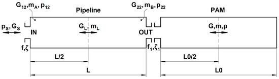
Figure 3.
System «Pipeline—PAM as object with lumped parameters».
The equations of the pressure change p’ and the mass flow rate m’ in the bladder, without taking into account the wave processes, are expressed as
This mathematical model consists of Equations (4), (5), (13), (18), (20–22), (28), and (29) and is designated as Model 2. The system of equations is presented in Appendix B (Equation (A2)).
3. Results
The numerical investigations were carried out to examine the impact of the parameters of the PAM and the supply pipeline in addition to a PWM frequency on the pressure change at the end of the bladder. The values of constant parameters are given below in Table 2.
Table 2.
Constant parameters for simulation.
Consider a PWM signal of the control on–off valve as a periodically time-varying pressure pS:
where pS0 is the pressure delivered from the air compressor, n is the operating frequency of the valve, pA is the atmospheric pressure.
3.1. Numerical Results of the Pressure Change at the End of the PAM
3.1.1. Different Initial Lengths of the PAM Bladder
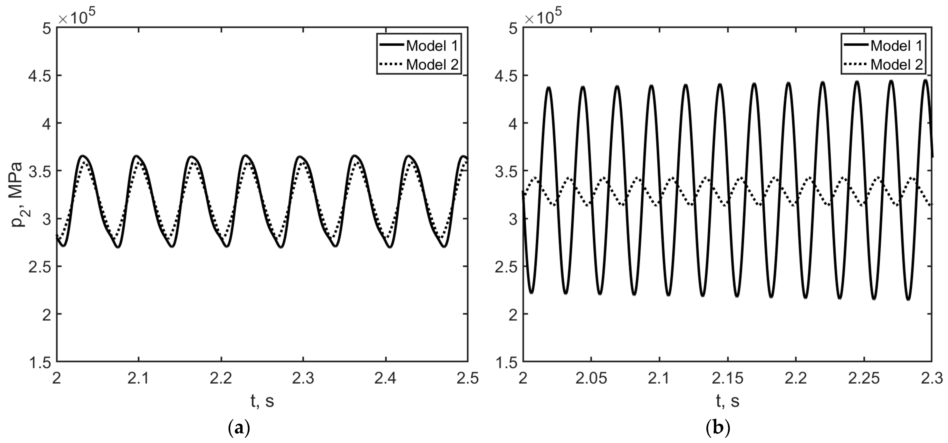
In Figure 4, the calculation results of the pressure change at the end of the PAM bladder in the case of the different initial bladder lengths L0 are shown. The results are obtained from Model 1 and Model 2 for the following initial parameters: L0 equal to 1 m and 2 m, D0 equal to 0.01, ζ1 and ζ2 equal to 25, L equal to 2 m, DL equal to 0.01 m, d and d1 equal to 0.008 m, pS0 equal to 0.5 MPa, n equal to 40 Hz.

Figure 4.
The pressure change at the end of the PAM: (a) L0 = 1 m; (b) L0 = 2 m.
From the analysis of the results, it can be stated that the bladder length has a significant influence on the gas oscillations. Figure 4b shows that the amplitude of the pressure change oscillations obtained from Model 1 exceed the amplitude obtained from Model 2 by 240%. When comparing Figure 4a,b, it can be seen that a significant discrepancy between simulation results obtained from Model 1 and Model 2 occurs. Therefore, correction of the valve operating frequency is necessary.
3.1.2. Different Lengths of the Supply Pipeline
Figure 5 illustrates the influence of the length of the supply pipeline on the wave processes in the bladder.

Figure 5.
The pressure change at the end of the PAM: (a) L = 0.5 m; (b) L = 2 m.
The pipeline length L is equal to 0.5 m and to 2 m, the diameter of the pipeline DL is equal to 0.01 m, the initial diameter of the bladder D0 is equal to 0.01 m, the initial length of the bladder L0 is equal to 2 m, the resistance coefficients ζ1 and ζ2 are equal to 25, the diameters of the pipeline d and the PAM inlet d1 are equal to 0.008 m, the pressure pS0 is equal to 0.5 MPa, the operating frequency n is equal to 40 Hz.
The simulation results presented on Figure 5a,b show that the pressure change at the end of the bladder being stronger depends on the length of the connected pipeline. According to Figure 5a, one can conclude that for a certain combination of parameters, the discrepancy between the amplitudes of the pressure change obtained from Model 1 and Model 2 can achieve 360%.
3.1.3. Different Operating Frequencies
In order to investigate the impact of the valve operating frequency, the calculations were carried out with the operation frequency n equal to 15 Hz and 40 Hz and the initial diameter D0 and the length L0 of the bladder equal to 0.04 m and 1 m, respectively. The other parameters have the following values: L = 1 m, DL = 0.02 m, ζ1 = ζ2 = 18, d = d1 = 0.016 m, pS0 = 0.5 MPa. In Figure 6, the simulation results are presented.

Figure 6.
The pressure change at the end of the PAM: (a) n = 15 Hz; (b) n = 40 Hz.
The resulting curves presented in Figure 6b obtained from Model 1 and Model 2 also show the inappropriate divergence between the amplitudes of the pressure change oscillations, which is equal to 500%. From the comparison of results presented in Figure 6a,b, it can be seen that the elaborated model allows predicting undesirable PWM frequencies that can lead to resonant gas oscillations and correcting them further.
3.2. Numerical Results of the Pressure Force at the End of the PAM
To calculate the pressure force at the end of the PAM bladder, the following equations were added to Model 1 and Model 2, respectively [50]:
where F2 and p2 are the pressure force and the pressure at the end of the bladder according to Figure 2, and F and p are the pressure force and the pressure at the end of the bladder according to Figure 3.
The simulation results are obtained for the following parameters: DL = 0.01 m, L = 1 m, D0 = 0.01 m, L0 = 2 m, d = d1 = 0.008 m, ζ1 = ζ2 = 25, pS0 = 0.5 MPa, n = 40 Hz.
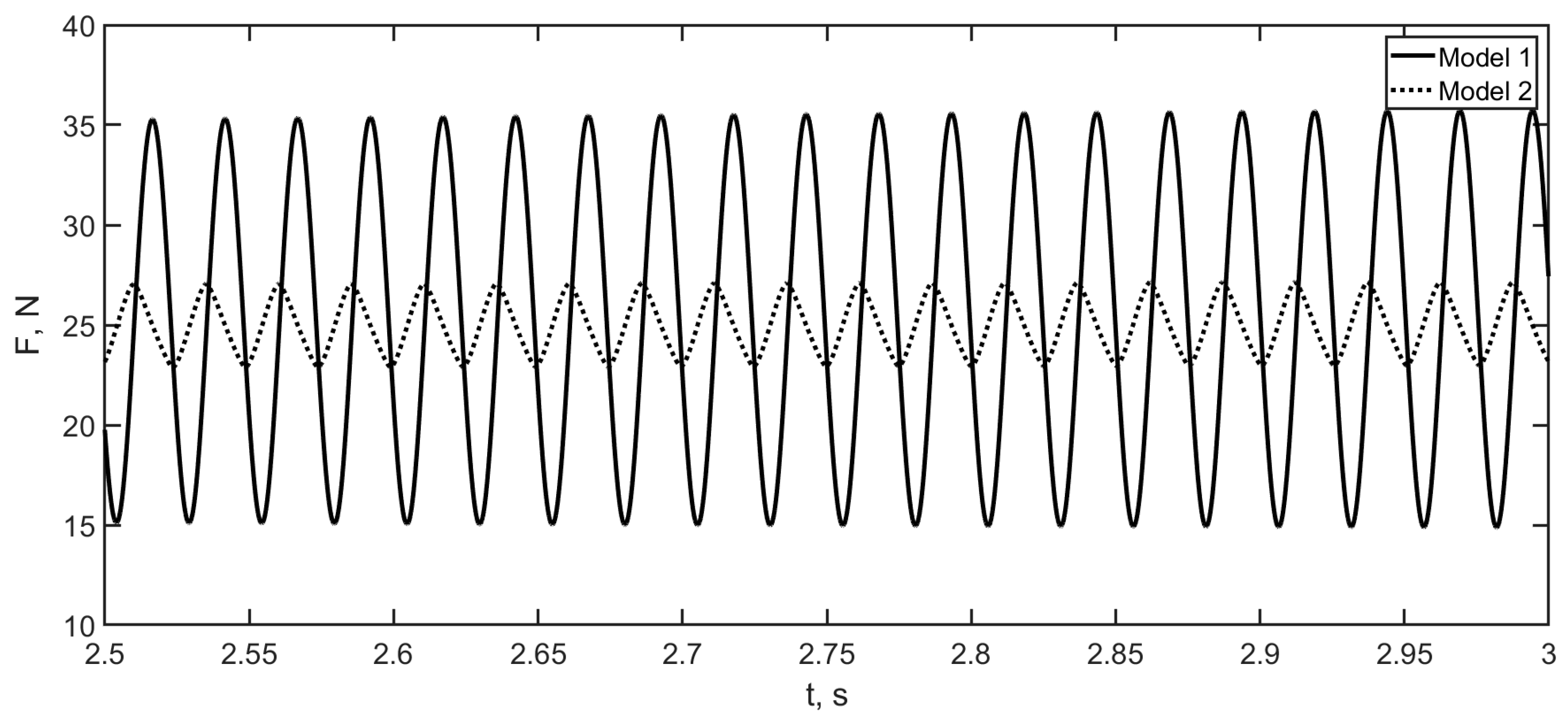
The pressure force curves at the end of the bladder are presented in Figure 7.

Figure 7.
The pressure force at the end of the PAM bladder.
As shown in Figure 7, the divergence between the amplitude of the pressure force oscillations obtained from Model 1 and the amplitude of the pressure force oscillations obtained from Model 2 is equal to 300%.
It can be concluded from Figure 4, Figure 5, Figure 6 and Figure 7 that the presented model enables us to define the working regime in which the wave processes and the oscillations of the pressure can occur. Also, the elaborated models allow determining the conditions under which it is necessary to take into account the pressure change in the connected pipeline.
3.3. The Calculation Algorithm
During the design of a PAM-actuated system with PWM signal control, the following algorithm can be applied:
- Step 1. Calculate the pressure change at the end of the bladder with Model 1 (Equation (A1)), taking into account the length and diameter of the bladder and the pipeline.
- Step 2. Calculate the pressure change at the end of the bladder with Model 2 (Equation (A2)), eliminating the wave processes in the bladder.
- Step 4. If the discrepancy between the results is large, then correction of the frequency of the PWM signal is required. Correct the valve operating frequency to eliminate the discrepancy until the curves match.
- Step 5. Then, continue the calculations using the models of the PAMs that take into account change in the design parameters, for example, with the model elaborated in [41] that describes static and dynamic characteristics of the PAM.
4. Conclusions
Mathematical models of the PAM elaborated earlier by the different authors allow calculating static and dynamic characteristics of the system actuated by pneumatic artificial muscles. However, when designing a pneumatic PAM-actuated system with PWM-based position control, it is necessary to take into consideration the wave processes in the gas flow inside the PAM bladder. These processes can lead to output link vibrations and can have a negative impact on the work of the whole system. These mathematical models consider the PAM as an object with lumped parameters and do not take into account change in the gas parameters along the bladder length.
The main result of our work is the elaborated distributed parameter model of the PAM. The advantages of the presented model are as follows:
- It allows estimating dynamic characteristics of the pressure change at the end of the bladder and avoiding undesirable PWM frequencies.
- It takes into consideration the wave processes in the supply pipeline, since the pipeline length can reach large values.
- It consists of ODEs instead of PDEs, which simplifies the calculations of dynamic characteristics.
- This model is universal for all types of PAMs since it consider the PAM as a pipeline.
It must be noted that the proposed model may have limitations in practical applications. The model does not take into account possible changes in temperature and the pressure in the bladder of the PAM. It may affect the accuracy of the numerical results. However, the experimental validation and correction of the proposed model would be the next step in our research and this will be the focus of future works.
Author Contributions
Conceptualization, A.D. and L.K.; methodology, A.D.; validation, L.K.; formal analysis, A.D. and L.K.; investigation, A.D. and L.K.; resources, A.Z.; data curation, A.Z.; writing—original draft preparation, L.K.; writing—review and editing, N.Z. and A.Z. All authors have read and agreed to the published version of the manuscript.
Funding
The research was partially funded by the Ministry of Science and Higher Education of the Russian Federation as part of the World-Class Research Center Program: Advanced Digital Technologies (contract no. 075-15-2022-311 dated 20 April 2022).
Data Availability Statement
The original contributions presented in the study are included in the article, further inquiries can be directed to the corresponding author.
Conflicts of Interest
The authors declare no conflicts of interest.
Abbreviations
| L | the length of the pipeline, m; |
| DL | the diameter of the pipeline, m; |
| VL | the value of the gas volume in the pipeline, m3; |
| fL | the cross-section area of the pipeline, m2; |
| f | the cross-section area of the pipeline inlet, m2; |
| d | the diameter of the pipeline inlet, m; |
| L0 | the initial length of the PAM, m; |
| D0 | the initial diameter of the PAM, m; |
| V0 | the value of the gas volume in the PAM, m3; |
| f0 | the cross-section area of the PAM, m2; |
| f1 | the cross-section area of the inlet of the PAM, m2; |
| d1 | the diameter of the PAM inlet, m; |
| pS | the supply pressure/the time-varying pressure, MPa; |
| pS0 | the pressure delivered from the air compressor, MPa; |
| pA | the atmospheric pressure, MPa; |
| pFR | the friction loss in the pipeline, MPa; |
| pFR0 | the friction loss in the PAM, MPa; |
| p12 | the pressure down the inlet of the pipeline, MPa; |
| p22* | the current pressure at the end of the pipeline, MPa; |
| p220 | the initial pressure at the end of the pipeline, MPa; |
| p22 | the pressure characterizing the dynamics of gas layer compression at the end of the pipeline, MPa; |
| p1 | the pressure down the PAM inlet, MPa; |
| p2* | the current pressure at the end of the PAM, MPa; |
| p20 | the initial pressure at the end of the PAM, MPa; |
| p2 | the pressure characterizing the dynamics of gas compressing at the end of the PAM, MPa; |
| p | the pressure at the end of the bladder (lumped parameters), MPa; |
| F | the pressure force at the end of the bladder (lumped parameters), H; |
| F2 | the pressure force at the end of the bladder (distributed parameters), H; |
| t | the time of the wave propagation, s; |
| c | the speed of the sound, m/s; |
| TS | the gas temperature in the pipeline and in the bladder, K; |
| R | the gas constant, J/kg·K; |
| k | the polytropic coefficient; |
| λ | the air resistance coefficient; |
| ρ | the average gas density in the pipeline, kg/m3; |
| ρ0 | the average gas density in the PAM, kg/m3; |
| υ | the average speed of the gas of the pipeline, m/s; |
| υ’ | the acceleration of the gas mass in the pipeline, m/s2; |
| υ0 | the average speed of the gas in the PAM, m/s; |
| the acceleration of the gas mass in the PAM, m/s2; | |
| ζ | the resistance coefficient of the pipeline inlet; |
| ζ1 | the resistance coefficient of the PAM inlet; |
| n | the operating frequency of the valve, Hz; |
| GL | the average mass flow rate in the pipeline, m3/s; |
| GS | the mass flow rate at the inlet of the pipeline, m3/s; |
| mL | the current value of the gas mass in the pipeline, kg; |
| mA | the current value of the gas mass at the inlet of the pipeline, kg; |
| mB | the current value of the gas mass at the outlet of the pipeline, kg; |
| m12 | the current value of the gas mass in the left half of the pipeline, m3/s; |
| the mass flow rate in the left half of the pipeline, m3/s; | |
| m22 | the current value of the gas mass in the second half of the pipeline, m3/s; |
| the mass flow rate in the second half of the pipeline, m3/s; | |
| m’A, G12 | the mass flow rate down the inlet of the pipeline, m3/s; |
| m’B, G22 | the mass flow rate at the outlet of the pipeline, m3/s; |
| m’, G | the average mass flow rate in the PAM, m3/s; |
| G1 | the mass flow rate down the inlet of the PAM, m3/s; |
| m | the current value of the gas mass in the PAM, kg; |
| the Heaviside step function |
Appendix A
Table A1.
The chronology of PAM mathematical models.
Table A1.
The chronology of PAM mathematical models.
| Authors | Year | Description of the Model | Type of Model | Type of PAM |
|---|---|---|---|---|
| Gaylord R.H. [34] | 1958 | elaborated the basic equation using the principle of energy conservation | geometric | McKibben |
| Schulte H.F. [35] | 1961 | geometric | McKibben | |
| Chou C.-P. and Hannaford B. [25] | 1996 | added wall thickness of bladder to the basic equation in [31] | geometric | McKibben |
| Repperger D.W. et al. [51] | 1998 | presented model consisting of a spring element, viscous damping element, contractile force element arranged in parallel | phenomenological | McKibben |
| Tondu B. and Lopez P. [5] | 2000 | proposed the equation equivalent to [23]; added empirical parameter k(p); elaborated the friction model | geometric empirical | McKibben |
| Tsagarakis N., Caldwell D.G. [36] | 2000 | considered the geometry of the end-cap surface; calculated radial elasticity | geometric | McKibben |
| Klute G.K. and Hannaford B. [37] | 2000 | considered elastic energy storage in the bladder | phenomenological | McKibben |
| Colbrunn R.W. et al. [56] | 2001 | elaborated the model consisting of a spring, viscous damper, and Coulomb friction arranged in parallel | phenomenological | McKibben |
| Hesse S. [42] | 2003 | proposed the equation of the static force | geometric | FESTO |
| Reynolds D.B. et al. [55] | 2003 | improved and experimentally tested the model in [47] | phenomenological | McKibben |
| Davis S. et al. [38] | 2003 | considered extension of the fiber strand | geometric | McKibben |
| Hildebrandt A. et al. [43] | 2005 | a pneumatic artificial muscle is proposed as combination of a pneumatic piston and mechanical spring | empirical | FESTO |
| Davis S. et al. [40] | 2006 | proposed the braid strands stress analysis; improved the friction model presented in [5] | geometric | McKibben |
| Kerscher T. et al. [44] | 2006 | added empirical function μ(p) in the equation in [5] | geometric empirical | FESTO |
| Doumit M. et al. [39] | 2009 | presented a fully analytical static model; considered the muscle end-fixture-diameter effect | geometric | McKibben |
| Wickramatunge K.C., Leephakpreeda T. [45] | 2010 | a pneumatic artificial muscle is modeled as a spring system and static force is presented as a function of stiffness and stretched length | empirical | FESTO |
| Joupilla V.T. [46] | 2010 | the static force is presented as a function of length contraction and the pressure and deducted from the maximum muscle force | empirical | FESTO |
| Pujana A.A. et al. [47] | 2010 | the static force is presented as a linear function of the internal pressure and length | empirical | FESTO |
| Hosovsky A. Havran M. [48] | 2012 | presented an approximation model of the static force using a polynomial function | empirical | FESTO |
| Sarosi J. et al. [49] | 2015 | presented an approximation model of the static force using an exponential function | empirical | FESTO |
| Donskoj et. al. [50] | 2019 | proposed an equation of the static force and a mathematical model of dynamic characteristics | geometric empirical | FESTO |
Appendix B
Model 1 looks as follows:
Model 2 looks as follows:
References
- Ahn, K.K.; Chau, N.U.T. Intelligent switching control of pneumatic muscle robot arm using learning vector quantization neural network. Mechatronics 2007, 17, 255–262. [Google Scholar] [CrossRef]
- Dolgih, E.V. Manipulator for Performance of Operations Related to Changing the Purpose of the Processing or Product in the Space. RU Patent 118 578 U1, 27 July 2012. [Google Scholar]
- Zhu, X.; Tao, G.; Yao, D.; Cao, J. Adaptive robust posture control of a parallel manipulator driven by pneumatic muscles. Automatica 2009, 44, 2248–2257. [Google Scholar] [CrossRef]
- Tondu, B.; Lopez, P. The McKibben muscle and its use in actuating robot-arms showing similarities with human arm behaviour. Ind. Robot. Int. J. 1997, 24, 432–439. [Google Scholar] [CrossRef]
- Tondu, B.; Lopez, P. Modelling and control of McKibben artificial muscle robot actuators. IEEE Contr. Syst. Mag. 2000, 20, 15–38. [Google Scholar] [CrossRef]
- Verrelst, B.; Vanderborght, B.; Van Ham, R.; Daerden, F.; Lefeber, D.; Vermeulen, J. The pneumatic biped “Lucy” actuated with pleated pneumatic artificial muscles. Auton. Robot. 2005, 18, 201–213. [Google Scholar] [CrossRef]
- Noritisugu, T.; Tanaka, T. Application of rubber artificial muscle manipulator as a rehabilitation robot. IEEE/ASME Trans. Mechatron. 1997, 2, 259–267. [Google Scholar] [CrossRef]
- Belforte, G.; Eula, G.; Ivanov, A.; Sirolli, S. Soft pneumatic actuators for rehabilitation. Actuators 2014, 3, 84–106. [Google Scholar] [CrossRef]
- Chi, H.; Su, H.; Liang, W.; Ren, Q. Control of a Rehabilitation Robotic Device Driven by Antagonistic Soft Actuators. Actuators 2021, 10, 123. [Google Scholar] [CrossRef]
- Nguyen, H.T.; Trinh, V.C.; Le, T.D. An Adaptive Fast Terminal Sliding Mode Controller of Exercise-Assisted Robotic Arm for Elbow Joint Rehabilitation Featuring Pneumatic Artificial Muscle Actuator. Actuators 2020, 9, 118. [Google Scholar] [CrossRef]
- Nguyen, T.; Leavitt, J.; Jabbari, F.; Bobrow, J. Accurate sliding-mode control of pneumatic system using low-cost solenoid valves. IEEE/ASME Trans. Mechatron. 2007, 12, 216–219. [Google Scholar] [CrossRef]
- Xie, S.; Mei, J.; Liu, H.; Wang, P. Motion control of pneumatic muscle actuator using fast switching valve. In Mechanism and Machine Science; Springer: Singapore, 2017; pp. 1439–1451. [Google Scholar] [CrossRef]
- Lin, Z.; Wei, Q.; Ji, R.; Huang, X.; Yuan, Y.; Zhao, Z. An electro-pneumatic force tracking system using fuzzy logic based volume flow control. Energies 2019, 12, 4011. [Google Scholar] [CrossRef]
- Shin, M.C.; Ma, M.A. Position control of a pneumatic rodless cylinder using sliding mode MD-PWM control the high speed solenoid valves. JSME Int. J. Ser C Mech. Elem. Manuf. 1998, 41, 236–241. [Google Scholar] [CrossRef]
- Ahn, K.; Yokota, S. Intelligent switching control of pneumatic actuator using on/off solenoid valves. Mechatronics 2005, 15, 683–702. [Google Scholar] [CrossRef]
- Chen, Y.; Zhang, J.-F.; Yang, C.-J.; Niu, B. Design and hybrid control of the pneumatic force-feedback systems for arm-exoskeleton by using on/off valve. Mechatronics 2007, 17, 325–335. [Google Scholar] [CrossRef]
- Najjari, B.; Barakari, S.; Mohammadi, A.; Futohi, M.; Bostanian, M. Position control of an electro-pneumatic system based on PWM technique and FLC. ISA Trans. 2014, 53, 647–657. [Google Scholar] [CrossRef]
- Hodgson, S.; Tavakoli, M.; Pham, M.; Leleve, A. Nonlinear discontinuous dynamics averaging and PWM-based sliding control of solenoid-valve pneumatic actuators. IEEE/ASME Trans. Mechatron. 2015, 20, 876–888. [Google Scholar] [CrossRef]
- Lin, Z.; Zhang, T.; Xie, Q.; Wei, Q. Intelligent electro-pneumatic position tracking system using improved mode-switching sliding control with fuzzy nonlinear gain. IEEE Access 2018, 6, 34462–34476. [Google Scholar] [CrossRef]
- Leephakpreeda, T. Fuzzy logic based PWM control and neural controlled-variable estimation of pneumatic artifical muscle actuators. Expert. Syst. Appl. 2011, 38, 7837–7850. [Google Scholar] [CrossRef]
- Jouppila, V.T.; Gadsden, S.A.; Bone, G.M.; Ellman, A.U.; Habibi, S.R. Sliding mode control of a pneumatic muscle actuator system with a PWM strategy. Int. J. Fluid Power 2014, 15, 19–31. [Google Scholar] [CrossRef]
- Pipan, M.; Harakovic, N. Closed-loop volume flow control algorithm for fast switching pneumatic valves with PWM signal. Control Eng. Pract. 2018, 70, 114–120. [Google Scholar] [CrossRef]
- Rimar, M.; Fedak, M.; Corny, I.; Kulikov, A.; Kuna, S.; Kulikova, O.; Vahovsky, J. Pulse width modulation modelling for efficient pneumatic artificial muscle control. Adv. Mech. Eng. 2019, 11, 1687814019895439. [Google Scholar] [CrossRef]
- Pipan, M.; Herakovic, N. Volume flow characterization of PWM-controlled fast-switching pneumatic valves with PWM signal. Stroj. Vestn. J. Mech. Eng. 2016, 62, 543–550. [Google Scholar] [CrossRef]
- Chou, C.P.; Hannaford, B. Measurement and modelling of McKibben pneumatic artificial muscle. IEEE Trans. Robot. Autom. 1996, 6, 90–102. [Google Scholar] [CrossRef]
- Sheikh, S.M.; Sadigh, M.J.; Zareinejad, M. Precise dynamic modeling of pneumatic muscle actuators with modified Bouw–Wen hysteresis model. Proc. Inst. Mech. Eng. Part E J. Process Mech. Eng. 2021, 235, 1449–1457. [Google Scholar] [CrossRef]
- Fluidic Muscle DMSP/MAS. Available online: https://www.festo.com/rep/en_corp/assets/pdf/info_501_en.pdf (accessed on 20 March 2024).
- Bergemann, D.; Lorenz, B.; Thallemer, A. Actuating Means. U.S. Patent 6,349,746 B1, 26 February 2002. [Google Scholar]
- Takosoglu, J.E.; Laski, P.A.; Blasiak, S.; Bracha, S.; Bracha, G.; Pietrala, D. Determining the static characteristics of pneumatic muscles. Meas. Control 2016, 49, 62–71. [Google Scholar] [CrossRef]
- Takagi, T.; Sakaguchi, Y. Pneumatic Actuator for Manipulator. U.S. Patent 4,615,260 A, 7 October 1986. [Google Scholar]
- Kalita, B.; Leonessa, A.; Dwivedy, S.K. A review on the development of pneumatic artificial muscle actuators: Force model and application. Actuators 2022, 11, 288. [Google Scholar] [CrossRef]
- Daerden, F.; Lefeber, D. Pneumatic artificial muscles: Actuators for robotics and automation. Eur. J. Mech. Environ. Eng. 2002, 47, 11–21. [Google Scholar]
- Oguntosin, V.; Akindele, A. Design and characterization of artificial muscles from wedge-like pneumatic soft modules. Sens. Actuators A Phys. 2019, 297, 111523. [Google Scholar] [CrossRef]
- Gaylord, R.H. Fluid Actuated Motor System and Stroking Device. U.S. Patent 2,844,126 A, 22 July 1958. [Google Scholar]
- Schulte, H.F. The characteristics of the McKibben artificial muscle. In The Application of External Power in Prosthetics and Orthotics; National Academy of Sciences-National Research Council: Washington, DC, USA, 1961; pp. 94–115. [Google Scholar]
- Tsagarakis, N.; Caldwell, D.G. Improved modelling and assessment of pneumatic muscle actuators. In Proceedings of the 2000 ICRA. Millennium Conference, IEEE International Conference on Robotics and Automation, Symposia Proceedings (Cat. No.00CH37065), San Francisco, CA, USA, 24–28 April 2000; Volume 4, pp. 3641–3646. [Google Scholar] [CrossRef]
- Klute, G.K.; Hannaford, B. Accounting for elastic energy storage in McKibben artificial muscle actuators. J. Dyn. Sys. Meas. Control 2000, 122, 386–388. [Google Scholar] [CrossRef]
- Davis, S.; Tsagarakis, N.; Canderle, J.; Caldwell, D.G. Enhanced modelling and performance in braided pneumatic muscle actuators. Int. J. Robot. Res. 2003, 22, 213–227. [Google Scholar] [CrossRef]
- Doumit, M.; Fahim, A.; Munro, M. Analytical modeling and experimental validation of the braided pneumatic muscle. IEEE Trans. Robot. 2009, 25, 1282–1291. [Google Scholar] [CrossRef]
- Davis, S.; Caldwell, D.G. Braid effects on contractile range and friction modeling in pneumatic muscle actuators. Int. J. Robot. Res. 2006, 25, 359–369. [Google Scholar] [CrossRef]
- Kotkas, L.; Zhurkin, N.; Donskoy, A.; Zharkovsky, A. Design and mathematical modeling of a pneumatic artificial muscle-actuated system for industrial manipulators. Machines 2022, 10, 885. [Google Scholar] [CrossRef]
- Hesse, S. The Fluidic Muscle in Application, 150 Practical Examples Using the Pneumatic Muscle; Blue Digest on Automation, Festo: Esslingen, Germany, 2003. [Google Scholar]
- Hildebrandt, A.; Sawodny, O. Cascaded control concept of a robot with two degrees of freedom driven by four pneumatic muscle actuators. In Proceedings of the 2005, American Control Conference, 2005, Portland, OR, USA, 8–10 June 2005; Volume 1, pp. 680–685. [Google Scholar] [CrossRef]
- Kerscher, T.; Albiez, J.; Zollner, J.M.; Dillmann, R. Evaluation of the dynamic model of fluidic muscles using quick-release. In Proceedings of the First IEEE/RAS-EMBS International Conference on Biomedical Robotics and Biomechatronics, BioRob 2006, Pisa, Italy, 20–22 February 2006; pp. 637–642. [Google Scholar] [CrossRef]
- Wickramatunge, K.C.; Leephakpreeda, T. Study on mechanical behaviours of pneumatic artificial muscle. Int. J. Eng. Sci. 2010, 48, 188–198. [Google Scholar] [CrossRef]
- Jouppila, V.T. Modelling and identification of a pneumatic muscle actuator system controlled by an on/off solenoid valve. In Proceedings of the 7th International Fluid Power Conference, Aachen, Germany, 22–24 March 2010; pp. 1–11. [Google Scholar]
- Pujana-Arrese, A.; Mendizabal, A.; Arenas, J.; Prestamero, R.; Landaluze, J. Modelling in Modelica and position control of a 1-DoF set-up powered by pneumatic muscles. Mechatronics 2010, 20, 535–552. [Google Scholar] [CrossRef]
- Hosovsky, A.; Havran, M. Dynamic modelling of one degree of freedom pneumatic muscle-based actuator for industrial applications. Teh. Vjesn. 2012, 19, 673–681. [Google Scholar]
- Sarosi, J.; Biro, L.; Nemeth, J.; Cveticanin, L. Dynamic modelling of a pneumatic muscle actuator with two-direction motion. Mech. Mach. Theory 2015, 85, 25–34. [Google Scholar] [CrossRef]
- Donskoj, A.S.; Kotkas, L.A.; Salova, T.P.; Barilovich, V.; Girshov, V.; Mertens, K.K.; Cherkesov, G.; Fokin, G.; Akhmetova, I.G. Modelling the static and dynamic characteristics of pneumatic muscle. IOP Conf. Ser. Earth Environ. Sci. 2019, 337, 012042. [Google Scholar] [CrossRef]
- Trojanova, M.; Hosovsky, A.; Cakurda, T. Evaluation of machine learning-based parsimonious models for static modelling of fluidic muscles in compliant mechanisms. Mathematics 2023, 11, 149. [Google Scholar] [CrossRef]
- Repperger, D.W.; Johnson, K.R.; Philips, C.A. A VSC position tracking system involving a large scale pneumatic muscle actuator. In Proceedings of the 37th IEEE Conference on Decision & Control (Cat. No.98CH36171), Tampa, FL, USA, 18 December 1998; Volume 4, pp. 4302–4307. [Google Scholar] [CrossRef]
- Serres, J.L.; Reynolds, D.B.; Philips, C.A.; Gerschutz, M.J.; Repperger, D.W. Characterization of a phenomenological model for commercial pneumatic muscle actuators. Comput. Methods Biomech. Biomed. Eng. 2009, 12, 423–430. [Google Scholar] [CrossRef]
- Kalita, B.; Dwivedy, S.K. Nonlinear dynamic response of pneumatic artificial muscle: A theoretical and experimental study. Int. J. Non-Linear Mech. 2020, 125, 103544. [Google Scholar] [CrossRef]
- Reynolds, D.B.; Repperger, D.W.; Phillips, C.A.; Bandry, G. Modelling the dynamic characteristics of pneumatic muscle. Ann. Biomed. Eng. 2003, 31, 310–317. [Google Scholar] [CrossRef]
- Colbrunn, R.W.; Nelson, G.M.; Quinn, R.D. Modelling of braided pneumatic actuators for robotic control. In Proceedings of the 2001, IEEE/RSJ International Conference on Intelligent Robots and Systems. Expanding the Societal Role of Robotics in the Next Millennium (Cat. No. 01CH37180), Maui, HI, USA, 29 October–3 November 2001; IEEE: Piscataway, NJ, USA, 2001; Volume 4, pp. 1964–1970. [Google Scholar] [CrossRef]
- Donskoy, A.S. Simulation of pressure fluctuations in pneumatic objects using ordinary differential equations. Izv. Vyss. Uchebnykh Zaved. Seriya Teknol. Tekst. Promyshlennosti 1997, 4, 94–97. [Google Scholar]
- Krichel, S.V.; Sawodny, O. Non-linear friction modelling and simulation of long pneumatic transmission lines. Math. Comput. Model. Dyn. Syst. 2013, 20, 23–44. [Google Scholar] [CrossRef]
- Stecki, J.S.; Davis, D.C. Fluid transmission lines—Distributed parameter models, part 1: A review of the state of the art. Proc. Inst. Mech. Eng. Part A 1986, 200, 215–228. [Google Scholar] [CrossRef]
- Stecki, J.S.; Davis, D.C. Fluid transmission lines—Distributed parameter models part 2: Comparison of models. Proc. Inst. Mech. Eng. Part A 1986, 200, 229–236. [Google Scholar] [CrossRef]
- Nikitin, N.V. Direct numerical modelling of three-dimensional turbulent flows in pipes of circular cross section. Fluid. Dynam. 1994, 29, 749–758. [Google Scholar] [CrossRef]
- Kern, R. Physical modelling of a long pneumatic transmission line: Models of successively defreasing complexity and their experimental validation. Math. Comput. Modell. Dyn. Syst. 2017, 23, 1–18. [Google Scholar] [CrossRef]
- Watton, J.; Tadmori, M. A comparison of techniques for the analysis of transmission line dynamics in electrohydraulic control systems. Appl. Math. Modell. 1988, 12, 457–466. [Google Scholar] [CrossRef]
- Makinen, J.; Piche, R.; Ellman, A. Fluid transmission line modelling using a variational method. J. Dyn. Syst. Meas. Control 2000, 122, 153–162. [Google Scholar] [CrossRef]
- Trukhanov, K.I. Methods for Designing Optimal Servo Pneumatic Devices for Controlling Systems with Liquid Working Media. Ph.D. Thesis, Moscow Bauman Moscow State Technical University, Moscow, Russia, 2019. [Google Scholar]
- Tseyrov, E.M. Issues of Gas Dynamics of Air Circuit Breakers; Gosenergoizdat, USSR: Moscow, Russia, 1961. [Google Scholar]
- Donskoy, A.S. Method of analytical calculation of processes in pneumatic pipelines. In Proceedings of the IX International Science and Technical Conference, Hydraulic Machines, Hydraulic Drives and Hydropneumatic Automation, Current State and Development Prospects, St. Petersburg, Russia, 7–8 June 2016; SpbPU: St. Petersburg, Russia, 2016; pp. 327–338. [Google Scholar]
- Gercz, E.V.; Krejnin, G.V. The Calculation of Pneumatic Actuators. Reference Manual; Mechanical engineering, USSR: Moscow, Russia, 1975. [Google Scholar]
- Shcherba, V.E.; Khait, A.; Pavlyuchenko, E.A.; Bulgakova, I.Y. Development and Research of a Promising Pumpless Liquid Cooling System for Reciprocating Compressors. Energies 2023, 16, 1191. [Google Scholar] [CrossRef]
Disclaimer/Publisher’s Note: The statements, opinions and data contained in all publications are solely those of the individual author(s) and contributor(s) and not of MDPI and/or the editor(s). MDPI and/or the editor(s) disclaim responsibility for any injury to people or property resulting from any ideas, methods, instructions or products referred to in the content. |
© 2024 by the authors. Licensee MDPI, Basel, Switzerland. This article is an open access article distributed under the terms and conditions of the Creative Commons Attribution (CC BY) license (https://creativecommons.org/licenses/by/4.0/).