Forecasting Electric Vehicles’ Charging Behavior at Charging Stations: A Data Science-Based Approach

Abstract

The rising adoption of electric vehicles (EVs), driven by carbon neutrality goals, has prompted the need for accurate forecasting of EVs’ charging behavior. However, this task presents several challenges due to the dynamic nature of EVs’ usage patterns, including fluctuating demand and unpredictable charging durations. In response to these challenges and different from previous works, this paper presents a novel and holistic methodology for day-ahead forecasting of EVs’ plugged-in status and power consumption in charging stations (CSs). The proposed framework encompasses data analysis, pre-processing, feature engineering, feature selection, the use and comparison of diverse machine learning forecasting algorithms, and validation. A real-world dataset from a CS in Boulder City is employed to evaluate the framework’s effectiveness, and the results demonstrate its proficiency in predicting the EVs’ plugged-in status, with XGBoost’s classifier achieving remarkable accuracy with an F1-score of 0.97. Furthermore, an in-depth evaluation of six regression methods highlighted the supremacy of gradient boosting algorithms in forecasting the EVs’ power consumption, with LightGBM emerging as the most effective method due to its optimal balance between prediction accuracy with a 4.22% normalized root-mean-squared error (NRMSE) and computational efficiency with 5 s of execution time. The proposed framework equips power system operators with strategic tools to anticipate and adapt to the evolving EV landscape.

1. Introduction

1.1. Motivation

In the pursuit of a sustainable and low-carbon future, the world is currently experiencing a transformative shift towards renewable energy sources and carbon neutrality, propelling electric vehicles (EVs) to the forefront of reliable and economically viable solutions for reducing greenhouse gas emissions [1]. This symbiotic relationship between the increasing adoption of renewable energy and the commitment to carbon neutrality not only curbs environmental impacts, but also catalyzes a revolutionary transformation of the transportation landscape [1]. An influential driver in the transition to cleaner transportation is the mandate established by the European Commission, which unequivocally stipulates that, by 2035, all the vehicles sold within Europe must be zero-emission vehicles [2]. This resolute directive underscores the urgency of embracing electric mobility and underscores the pivotal role EVs will play in reshaping the automotive sector. The exponential rise in EV adoption is not merely a projection, but a reality witnessed across continents [3]. Europe, in particular, has displayed remarkable growth, with EV sales in 2022 soaring with an annual growth rate of 15% compared to preceding years [1]. This trend is emblematic of a global shift toward sustainable transportation alternatives. Over the period from 2016 to 2021, China claimed the highest compound annual growth rate in EV adoption at 60%, trailed by the United States at 55% [1]. These figures underscore the global momentum toward EV integration.

Nonetheless, the evolution towards electric mobility is not devoid of challenges, especially concerning the seamless integration of EVs with the existing power grid. The unpredictability inherent in the charging behavior of EV users translates into significant fluctuations in power demand, potentially overburdening the power grid and leading to instances of grid congestion. This demand variability could also precipitate local transformer degradation, exacerbating the challenges in maintaining grid stability [4]. To fully exploit the benefits of the electric mobility revolution, accurate forecasting of EV charging behavior has emerged as an indispensable tool for harmonizing EV integration with the power grid. This proactive measure is essential for preventing grid congestion, optimizing energy distribution, and ensuring a consistent supply of electricity amidst the dynamic landscape of charging behaviors. Consequently, accurate forecasting of EV charging behavior has become a linchpin in effective power system planning, scheduling, and operation [5]. It facilitates the judicious management of EV charging stations (CSs), enabling optimal and secure management of power resources within the broader power ecosystem [6].

1.2. Background

The seamless integration of EVs into the power grid has required the development of accurate forecasting strategies to optimize the management of EV charging behavior [7,8,9]. Researchers have explored diverse methodologies to predict EV charging behavior, enabling effective grid management and enhanced energy utilization. An EV charging load prediction considering different types of EVs was developed by the authors in [10]. EV characteristics such as charging start time, charging session, initial state-of-charge (SoC), kilometers per day, and charging mode are analyzed in this EV charging prediction. Moreover, the GM (1, 1) model is used to estimate the EV owner behavior and to validate it by comparing the forecasting results with actual results obtained by simulation. The EV charging profiles obtained for each EV are clustered to create a total EV demand curve and then are compared with the real load curve. The results obtained show a significant accuracy to give guidance for the operation and planning considering EV integration into the grid. Even though the paper considered different types of EVs and charging characteristics in the modeling, it did not consider other important stages such as data pre-processing, feature engineering, and feature selection. A predictive model of EVs’ load consumption was developed in [11], utilizing both statistical and machine learning models, including Multiple Linear Regression (MLR), an Artificial Neural Network (ANN), Extreme Gradient Boosting (XGBoost), and Light Gradient Boosting Machine (LightGBM). EV energy consumption data from Aichi Prefecture, Japan, was utilized for the analysis, and three evaluation metrics—$R^2$, RMSE, and MAE—were employed to assess the performance of the forecasting models. Both XGBoost and LightGBM outperformed traditional models such as MLR and the ANN, with LightGBM outperforming XGBoost in terms of prediction accuracy. Despite including pre-processing, machine learning algorithms, and evaluation stages in their methodology, this paper did not consider the feature engineering and feature-selection stages, which are crucial for improving the forecasting results.

A methodology for predicting additional EV charging load in the mid-term and long-term was proposed by the authors in [12]. Using probabilistic modeling based on the Monte Carlo method, the authors analyzed EV charging profiles and forecasted future EV ownership patterns. The results unveiled insights, including the projected EV charging profile for 2025, forecasting an 11.08% increase in the existing load peak. However, despite comparing different probabilistic models, this methodology did not include data preparation, cleaning, or a feature-selection process to identify the most optimal variables to be used in the forecasting models. Lu et al. [13] harnessed the Random Forest (RF) algorithm to devise a forecasting strategy for EV charging load, focusing on short-term predictions for a single CS. Leveraging historical data, the RF algorithm provided an effective prediction for charging load, by combining the regression and classification algorithms and offering a robust solution for CSs. The results demonstrated an optimized Random Forest structure that achieved significantly small errors. Despite the practical application of the method developed and tested, the performance of Random Forest was not compared with other forecasting methods. Moreover, the forecasting performed by the authors considered only the EV charging load and left out the plugged-in status.

In [14], the authors proposed a forecasting model for CSs’ occupation considering the Markov chain model. Information such as the distribution of EVs at the charging station, the average time of connection, and energy consumed was used to obtain information about the occupancy model for a particular charging station and then to construe the charging profiles curve. Nevertheless, the proposed model was not trained to achieve a high resolution, nor to consider seasonal charging behavior to analyze different patterns, and it presented the limitation of the available data. A decentralized deep learning approach to reduce the waiting time of EV users of public CSs was proposed by the author in [15]. The main focus of this work was to predict the CSs’ occupancy by guaranteeing the privacy security of the CS operators since sensitive data that cannot be exposed to external entities are shared by the EV users. The decentralized deep learning model was based on an individual deep learning model to solve the problem for each CS and then was aggregated to deal with the information of all CSs.

In [16], the authors proposed the usage of historical charging data in conjunction with weather, traffic, and events data to predict EV session duration and energy consumption. They employed popular machine learning algorithms including RF, Support Vector Machine (SVM), XGBoost, and Deep Neural Networks. The results showed that the best predictive performance was achieved by an ensemble learning model, with SMAPE scores of 9.9% and 11.6% for session duration and energy consumption, respectively, highlighting the significance of traffic and weather information for charging behavior predictions. Nonetheless, the study did not forecast the plugged-in status. A hybrid predictive modeling approach for forecasting EV charging demand was introduced by the authors in [17], by merging the strengths of the Autoregressive Integrated Moving Average (ARIMA) and Artificial Neural Network (ANN) methodologies. The results indicated that machine learning techniques based on the proposed hybrid strategy outperformed existing statistical models, particularly RF, thereby improving accuracy in predicting charging demand. However, while the study emphasizes the importance of hybrid models in addressing the complexities of EV charging demand prediction, it did not include a feature-selection technique to determine the optimal features for the model.

Many research works have been focused on EV charging load prediction by considering aspects such as different types of EVs and implementing statistical methods and machine learning models [10,11]. Short-term, mid-term, and long-term EV charging load prediction approaches have been proposed by some authors [12,13].

Table 1. Main works addressing EV charging behavior forecasting.

Reference	Plugged-in Forecasting	Power Consumption Forecasting	Pre-Processing	Feature Engineering	Feature Selection	Forecasting Methods	Validation
[10]		✓					✓
[12]		✓		✓
[14]		✓
[13]		✓		✓	✓		✓
[11]		✓	✓			✓	✓
[16]		✓	✓	✓		✓	✓
[17]		✓	✓	✓		✓	✓
This work	✓	✓	✓	✓	✓	✓	✓

presents a summary of the main works related to EV charging behavior forecasting and compares the different components included in each paper with the contributions of this work.

1.3. Main Contributions

Considering the literature review, it is clear that there is a lack of papers devoted to considering important stages such as data preparation, cleaning, pre-processing, feature engineering, and feature selection even without considering seasonal charging behavior to evaluate different patterns, and consequently, there are the limitations of the available data. Recognizing these imperatives, this study presents a comprehensive computational methodology designed to predict EV charging behavior at CSs. This methodology considers the entire spectrum—from raw data analysis and transformation to pre-processing, feature engineering, feature selection, the utilization of diverse machine learning algorithms for forecasting, rigorous validation, and meticulous performance evaluation. The proposed framework establishes a structured pathway to augment the precision of EVs’ plugged-in status and power consumption predictions, thereby contributing to the seamless and sustainable integration of EVs into the evolving energy ecosystem.

In light of these studies, this paper seeks to enhance the domain of EV charging behavior prediction by proposing a novel and comprehensive methodology that stands out in its approach and scope. The key contributions of this work are listed as follows:

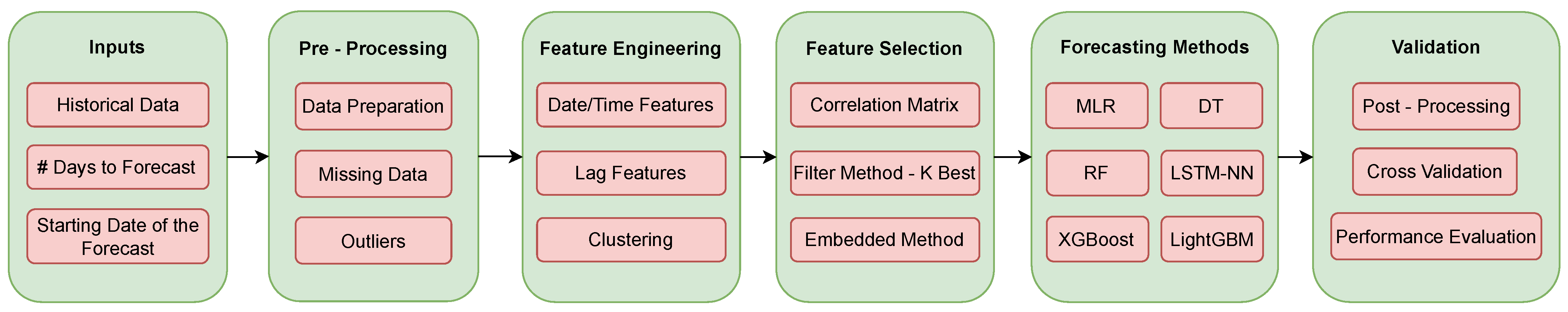
• Unlike many existing studies that focus solely on isolated aspects of forecasting, this methodology addresses the entire trajectory of EV charging behavior prediction. It bridges various stages, including data pre-processing, feature selection, and feature engineering, alongside the utilization and comparison of diverse forecasting methods, followed by a thorough validation and performance evaluation. This framework aims to harmonize and optimize every stage of the predictive process, enhancing the overall accuracy and reliability of EV charging behavior forecasting.
• This methodology places specific emphasis on forecasting both the plugged-in status and the power consumption of EVs at CSs, recognizing the significance of understanding both aspects for effective grid management. This is particularly important to determine the flexibility of the charging process, enabling the smart charging of the EVs.

1.4. Paper Organization

The rest of the paper is structured as follows. Section 2 describes the proposed methodology for EVs’ plugged-in status and power consumption forecasting, including the different stages. Section 3 presents a case study applying the methodology to a real-world dataset, including an in-depth analysis and discussion of the results. Section 4 summarizes the main outcomes of the paper.

2. Methodology

This section explains the methodology developed to forecast EVs’ plugged-in status and power consumption at CSs. The process, as shown in Figure 1, is composed of six stages: inputs, pre-processing, feature engineering, feature selection, forecasting methods, and validation. A detailed description of the entire methodology is presented to ensure the proposed approach can be fully replicated and understood, particularly in the context of forecasting EV charging behavior.

2.1. Inputs

The successful implementation and execution of the methodology requires the following inputs:

• Time series data:
  The initial dataset contains EVs’ charging sessions for a single CS. The data should include at least the following:
  Start date time (time stamp): The date and time at which the EV is connected for charging.
  End date time (time stamp): The date and time at which the EV is disconnected. It includes both the periods for which the EV is connected and actively charging and the periods for which the EV is connected, but no longer charging.
  Charging duration (minutes): The number of minutes the EV is connected and actively charging.
  Energy consumed (kWh): The amount of energy that has been dispensed by the CS to the EV during the charging session.
  The size of the dataset can vary, but the more data available, the better.
• Number of days to forecast:
  It is necessary to define the time horizon of the forecast (in days), e.g., 1 day, 7 days (a week), and 30 days (a month).
• Starting date of the forecast:
  It is necessary to define the starting date for the forecast period. All the data available before this date are used for training, and from this point onward, the specified number of days is forecasted.

2.2. Pre-Processing

In this section, the raw data from the dataset are first prepared and processed. They are then treated and cleaned by addressing missing data and outliers.

2.2.1. Data Preparation

Since the majority of open-access EVs’ charging datasets correspond to charging sessions (events) at the CSs, the initial step involves transforming the charging session data into a time series that captures the plugged-in status and power consumption every 15 min at the CS. The variable “plugged” is used to determine whether an EV is currently connected and actively charging during the given interval (1), or not (0). Meanwhile, the variable “power consumption” represents the cumulative power consumed (measured in kW) during that specific interval at the CS.

For the initial “start date time” of a charging session, combined with the “charging duration”, the “plugged-in” variable receives a value of 1, and the “energy consumed” is evenly distributed across that time span. In cases where multiple EVs are charging simultaneously, as indicated by the same time stamp (from other charging sessions), their energy consumption is aggregated. This process is iterated for all charging sessions.

Ultimately, any remaining time stamps that remain unfilled are allocated a “plugged-in” and “energy consumption” value of 0. This signifies that, during those specific time stamps, no EV was connected to the station, resulting in zero energy consumption.

The resulting final dataset is resampled to a 15 min data resolution, and the “energy consumption” values are converted into “power consumption”.

2.2.2. Missing Data

To address missing data, two approaches are employed:

• If the missing data gap consists of less than one hour of missing values, linear interpolation is utilized to bridge the gap. Linear interpolation is widely used in time series analysis and data imputation due to its simplicity and effectiveness [18] for handling short gaps of missing data.
• If the missing data gap spans over an hour of missing values, it remains unfilled. This decision is made to avoid introducing artificial values for extended time periods, which could potentially and adversely affect the accuracy of the forecasting process. However, in the dataset used in the present paper, the missing values are always lower than 1 h. For other datasets, the methods proposed in [18] can be applied.

2.2.3. Outliers

Detecting outliers in the context of EV power consumption at CSs is challenging due to the significant variability involved. Instances of both extremely high and remarkably low power consumption values can occur. This variability stems from a range of factors, including EV charging duration, the concurrent number of connected EVs, and the installed capacity of the CS.

Consequently, the sole circumstance under which a data point is classified as an outlier and subsequently removed from the dataset is when the $powerconsumption$ $\le 0$.

2.3. Feature Engineering

In this section, several useful features that can be utilized as inputs for the forecasting methods are generated. These features fall into two distinct categories: date/time features and lag features.

2.3.1. Date/Time Features

Date/time features refer to specific characteristics or attributes associated with dates and times. These features allow for time-based analysis, trend identification, pattern recognition, and the extraction of meaningful insights from temporal data. From the time stamp of each record, the following date/time features and their respective value ranges are generated:

• Week of year: 1–52.
• Day of year: 1–365.
• Season: 1–4 (winter = 1, spring = 2, summer = 3, fall = 4).
• Month: 1–12.
• Day of month: 1–30/31.
• Day of week: 1–7 (Monday-Sunday).
• Weekend: 1 if weekend, 0 if not.
• Holiday: 1 if holiday, 0 if not.
• Hour: 1–24.
• Minute: 15, 30 or 45.

2.3.2. Lag Features

Lag features, also known as time lag variables, are variables created by shifting or lagging past power observations. The lagged values are added as new features in conjunction with the original time series data. Each lagged feature represents the value of the original series at a specific time interval preceding the current observation. The subsequent lag features are established:

• Power lag 1: power consumption 1 day prior.
• Power lag 5: power consumption 5 days prior.
• Power lag 7: power consumption 7 days prior.

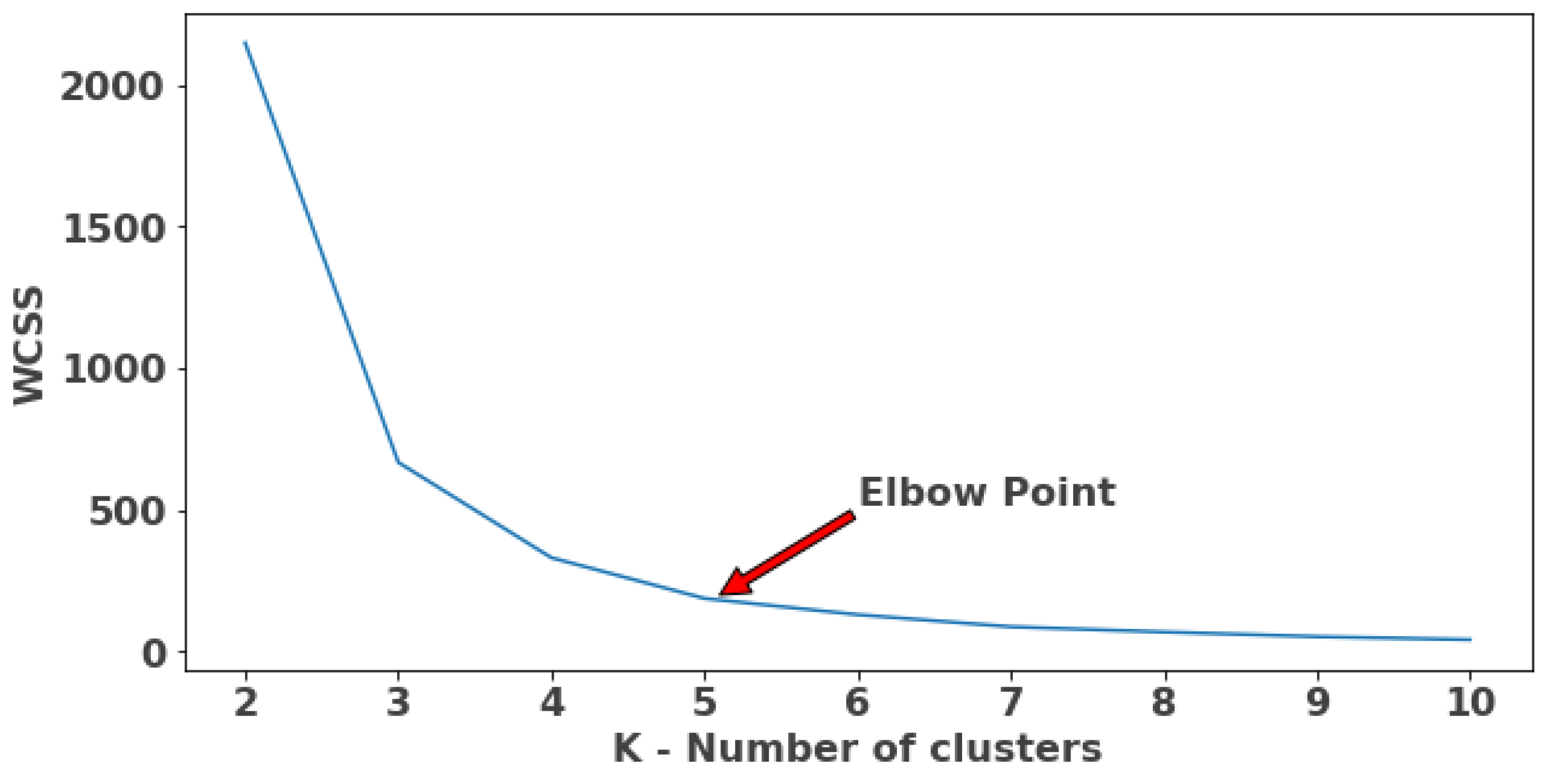
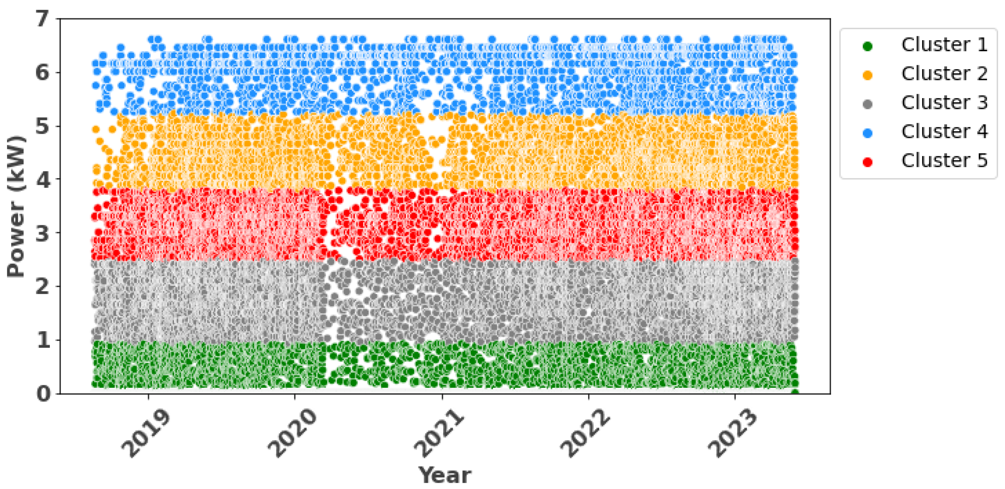
2.3.3. Clustering

A clustering process is performed with the purpose of identifying patterns or relationships between the EVs’ power consumption values at the CS. This entails categorizing the power consumption data points into clusters or groups using the K-means [19] method.

K-means is an unsupervised learning algorithm that groups data, based on each point’s Euclidean distance, to a central point called the centroid [20]. It aims to minimize the Within-Cluster Sum of Squares (WCSS), which represents the sum of squared distances between each data point and its centroid. Given a dataset with N data points and K clusters, the objective function for K-means clustering can be written as [21]:

$$WCSS=\sum _{k=1}^K\sum _{i=1}^N{r}_{ik}\left|\right|x_i-\overline{k}{\left|\right|}^2$$

(1)

where $r_{ik}$ is an indicator variable that denotes whether data point $x_i$ belongs to cluster k (1 if it belongs, 0 otherwise), $x_i$ represents the feature vector of data point i, $\overline{k}$ is the centroid of cluster k, and $\left|\right|x_i-\overline{k}{\left|\right|}^2$ denotes the Euclidean distance. The goal is to find the optimal values for $r_{ik}$ and $\overline{k}$ that minimize the WCSS.

To determine the optimal number of clusters K to use in K-means, the elbow method is used. It involves plotting the sum of squared distances (WCSS) against the number of clusters and looking for the “elbow” point on the graph [22]. The elbow point represents the value of K at which the incremental gain in clustering quality diminishes significantly. Sometimes, the elbow point may not be clear or easily identifiable.

Once the clusters (groups) are created, a new variable called cluster is generated assigning the cluster number to every power consumption data point. This new variable can also be employed as a feature within the forecasting methods.

2.4. Feature Selection

Feature selection is an integral process in machine learning involving the identification of pertinent features or variables from a dataset. The primary aim of feature selection is to curate a subset of features that hold the highest informativeness and influence in predicting the target variable. Consequently, this subset of features is utilized as the input in the forecasting methods.

Before selecting the features, it is essential to transform certain date/time features, such as week of year, day of year, season, month, day of month, day of week, hour, and minute. This transformation is imperative as these features inherently exhibit cyclic behavior. Therefore, each of these features is converted into two components (x and y) following the equations:

$$\begin{array}{c}\hfill f_x=sin(2\pi f/max(f\left)\right)\end{array}$$

(2)

$$\begin{array}{c}\hfill f_y=cos(2\pi f/max(f\left)\right)\end{array}$$

(3)

where f represents the cyclic feature to be transformed, $f_x$ and $f_y$ represent the first and second components of the cyclic feature, and $max\left(f\right)$ corresponds to the maximum value of the cyclic feature [16].

After the transformation of the cyclical features, a range of techniques and algorithms for feature selection is utilized to ascertain which features will be employed in the forecasting methods. These techniques include the correlation matrix, the filter method (K best), and the embedded method.

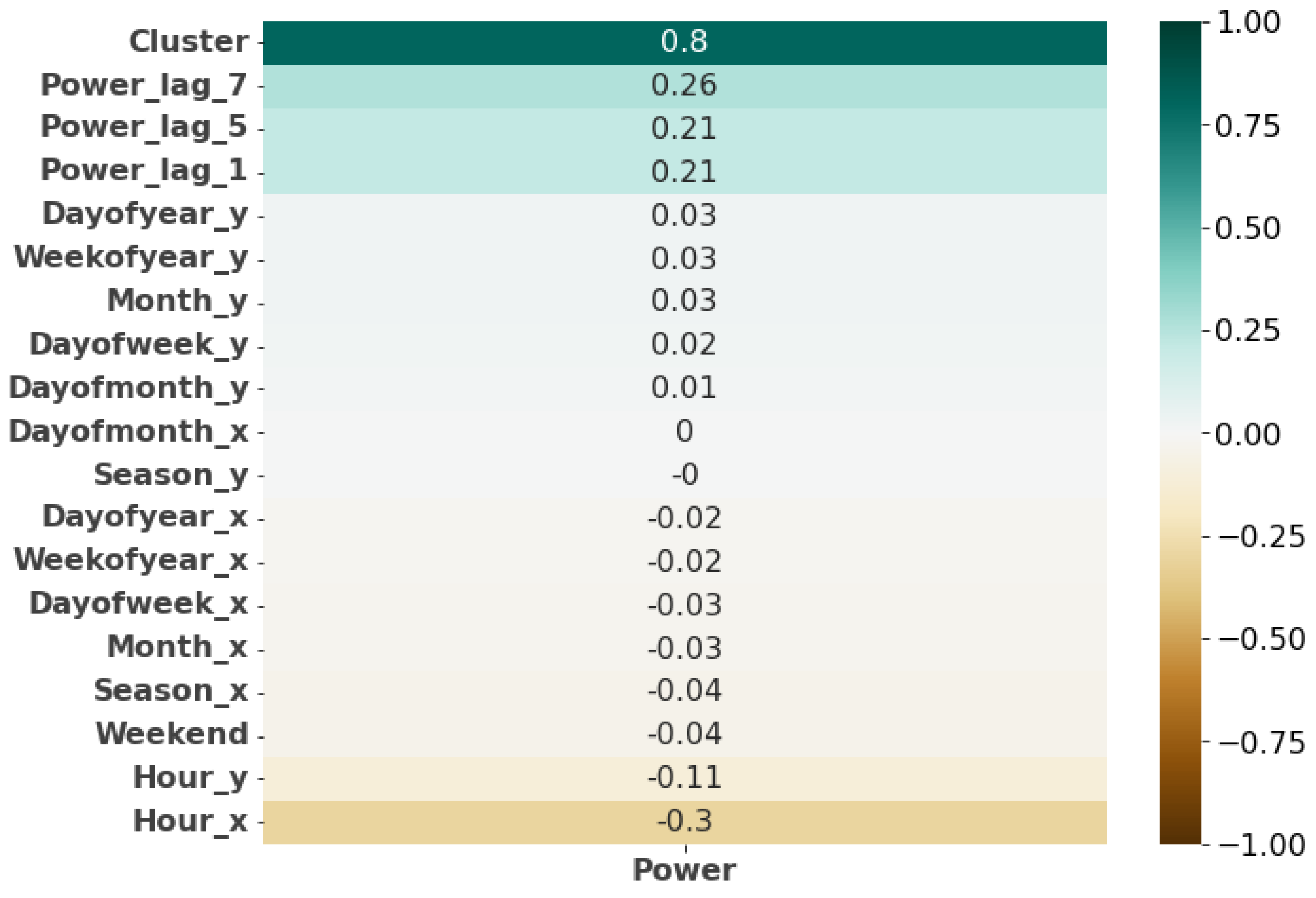
2.4.1. Correlation Matrix

The correlation matrix displays the pairwise correlations between variables within the dataset. It provides a quantitative measure of the strength and direction of the linear relationship between variables. Each cell in the matrix represents the Pearson correlation coefficient between two variables.

The correlation coefficient, typically denoted by r, ranges from −1 to 1. A positive value indicates a positive correlation, meaning that, as one variable increases, the other variable tends to increase as well [23]. Conversely, a negative value indicates a negative correlation, indicating that, as one variable increases, the other variable tends to decrease. A correlation coefficient of 0 suggests no linear relationship between the variables, and a correlation coefficient of 1 suggests a perfect linear relationship between the variables.

2.4.2. Filter Method: K Best

The filter method with the K best, also known as SelectKBest [24], is a feature-selection technique used in machine learning and data analysis that aims to select the K best features from a given dataset based on their statistical scores or relevance to the target variable.

The filter method evaluates each feature independently, without considering the relationship between features. It relies on statistical measures such as the chi-squared, ANOVA F-value, mutual information, or correlation coefficient to assign a score to each feature. After scoring each feature, SelectKBest selects the top K features with the highest scores and discards the rest. The value of K is determined by the user and represents the desired number of features to be selected.

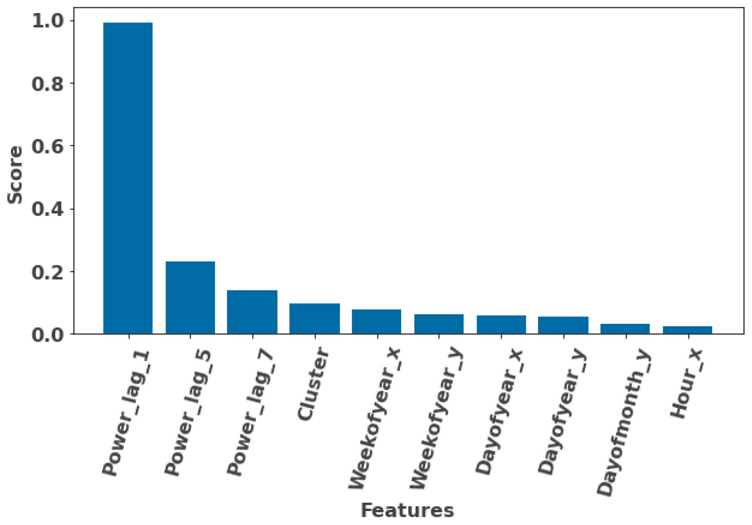
2.4.3. Embedded Method (Feature Importance)

The embedded method, specifically the technique of feature importance, is a feature-selection approach that incorporates feature selection directly into the process of training a machine learning model [24]. Unlike the filter method, which evaluates features independently of the learning algorithm, the embedded method considers the feature selection process as an integral part of the model training process.

Embedded methods determine feature importance by leveraging the inherent feature-selection capabilities of certain machine learning algorithms. These algorithms are designed to automatically assign weights or importance scores to each feature during the model training process. The importance scores reflect the impact of each feature on the model’s performance.

Common examples of machine learning algorithms that incorporate feature importance are tree-based models like Random Forest and Gradient Boosting Machines [25]. During the training process, these algorithms evaluate the relevance and contribution of each feature to the prediction task. The features that have a greater impact on the model’s performance are assigned higher importance scores, while less influential features are assigned lower scores.

2.5. Forecasting Methods

Six forecasting methods, namely Multiple Linear Regression (MLR), decision trees (DT), Random Forest (RF), the Long Short-Term Memory Neural Network (LSTM-NN), Extreme Gradient Boosting (XGBoost), and Light Gradient Boosting Machine (LightGBM) are evaluated in terms of their predictive performance for forecasting EVs’ power consumption at CSs. The selection of the regression methods was based on a comprehensive review of the existing literature on power consumption forecasting, and aimed to cover a range of traditional and modern machine learning methods, as well as deep learning techniques. MLR, being the simplest model, is used as a benchmark. Additionally, for the plugged-in status, the XGBoost classifier was employed to predict whether an EV will be connected (1) or not (0). The description of each forecasting method is provided below.

2.5.1. Multiple Linear Regression (MLR)

Linear regression is a statistical modeling technique used to establish a relationship between a dependent variable and one or more independent variables. It assumes a linear relationship between the variables, where the dependent variable can be predicted or explained by a linear combination of the independent variables [26]. The process involves fitting a linear regression model to the historical data and then using the model to make predictions.

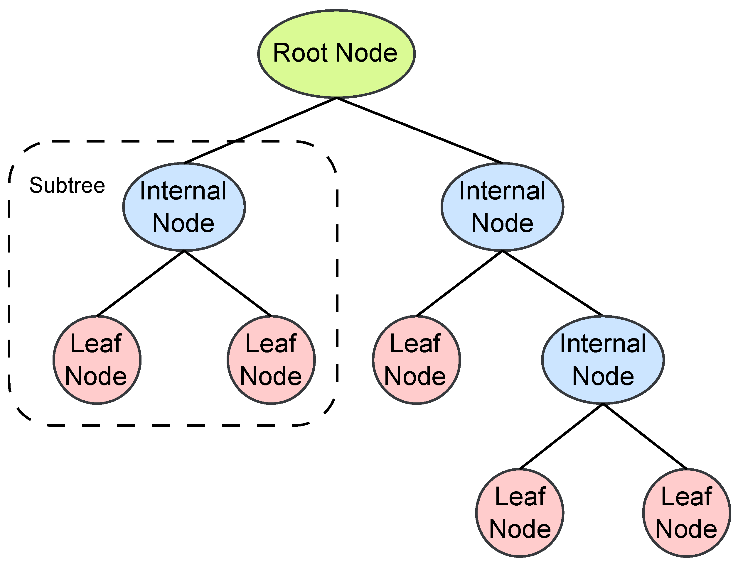
2.5.2. Decision Trees (DT)

DT is a machine learning algorithm for classification and regression tasks that uses a tree-like structure to represent a series of if–else decision rules to predict continuous numerical values. Unlike classification trees that predict class labels, regression trees predict numeric values based on the features of the input data. DT works by recursively partitioning the feature space based on selected features and split points [27]. Each internal node represents a decision rule based on a feature and split point, and each leaf node represents a prediction value or a class label.

The recursion to create child nodes continues until a stopping criterion is met, such as reaching a maximum depth, having a minimum number of instances in a node, or other criteria. The prediction for each leaf node is typically the average of the target variable values within that region. To make predictions for new instances, the algorithm traverses the decision tree based on the feature values of the instance until reaching a leaf node. The prediction value associated with that leaf node is used as the final prediction.

The general structure of DT is presented in Figure 2.

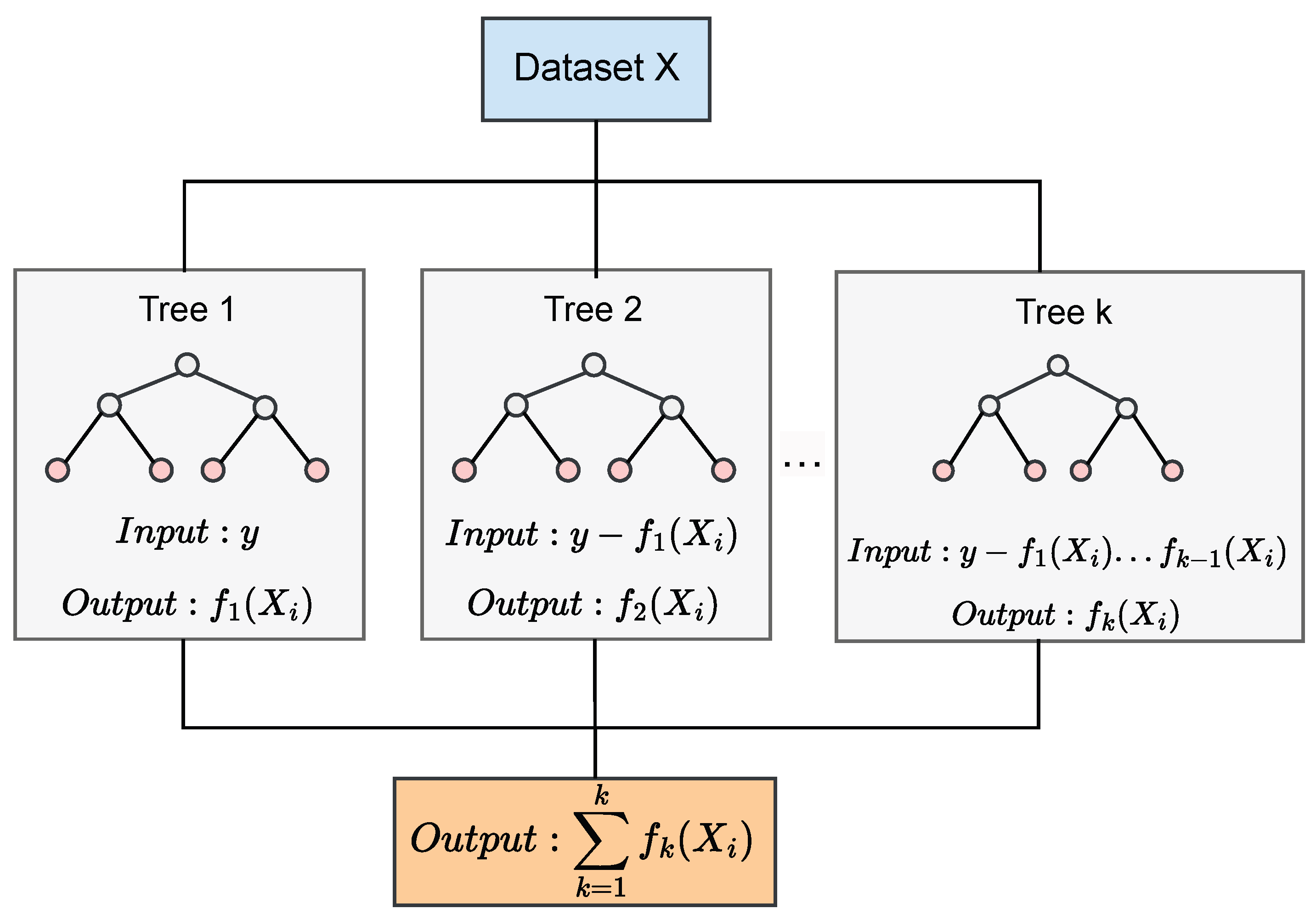
2.5.3. Random Forest (RF)

RF is an ensemble learning algorithm that combines multiple decision trees to perform classification and regression. To solve regression-based problems, RF uses the principle of averaging the predictions of individual trees to make the final prediction [28]. The construction of the RF algorithm for regression is composed by the following steps [29]:

• Parameters: $n\_estimators$ (number of decision trees to be included), $max\_depth$ (maximum depth allowed for each decision tree), and $min\_samples\_split$ (minimum number of samples required to split an internal node).
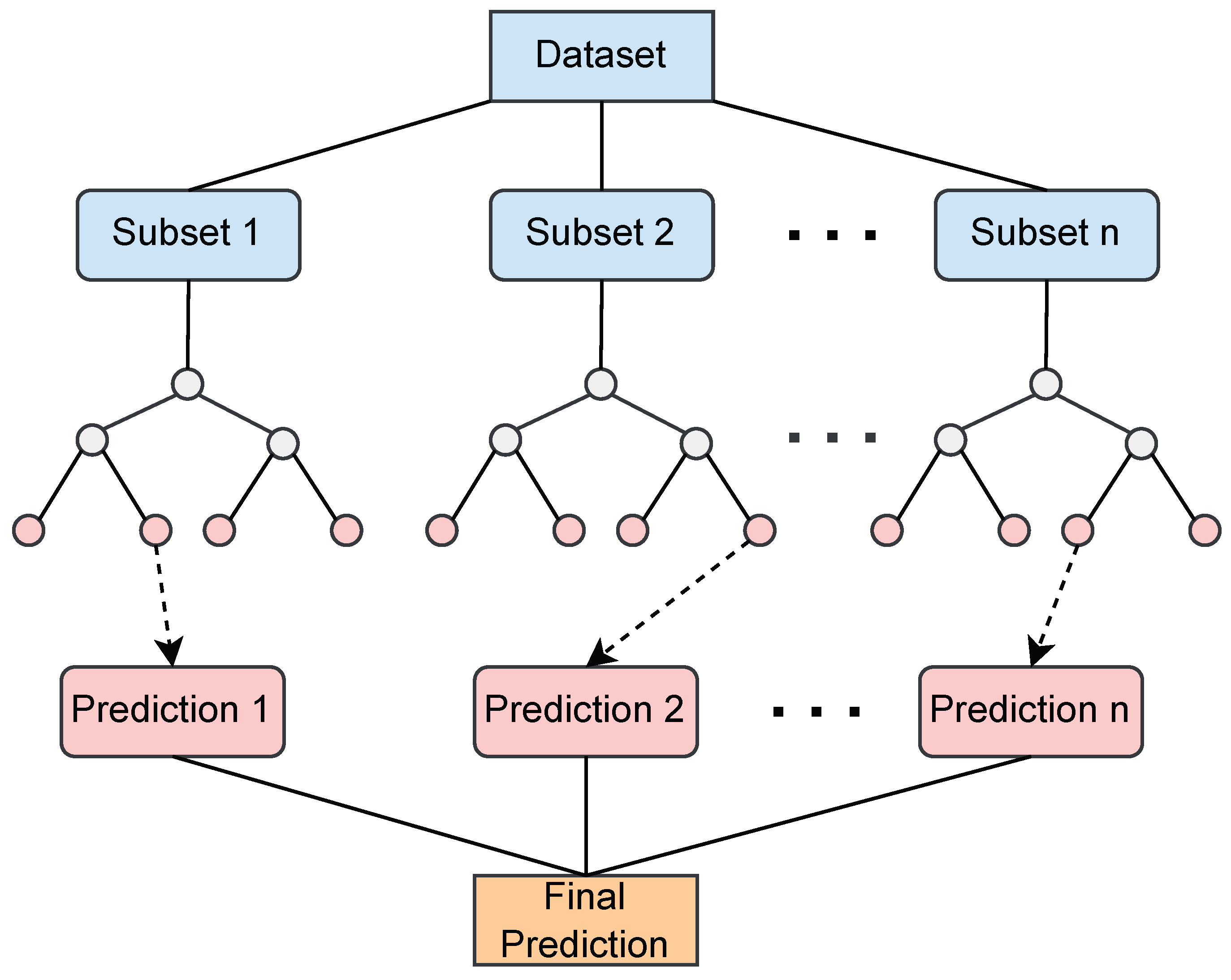
• Building of decision trees: Each decision tree in the RF is constructed using a subset of the original dataset. For each tree, a random subset of samples is selected with replacement, known as bootstrapping [30].
• Recursive binary splitting: If the stopping criterion is met (e.g., maximum depth reached or minimum number of samples for splitting not satisfied), a leaf node is created, and it is assigned the average target value of the samples in that node. Otherwise, the best feature and the split point that minimizes the mean-squared error (MSE) or any other splitting criterion are determined.
• Final prediction: Once all the decision trees are constructed, the predictions are made by aggregating the individual predictions from each tree, and the final prediction is obtained by averaging the predictions from all decision trees.

The general structure of RF can be seen in Figure 3.

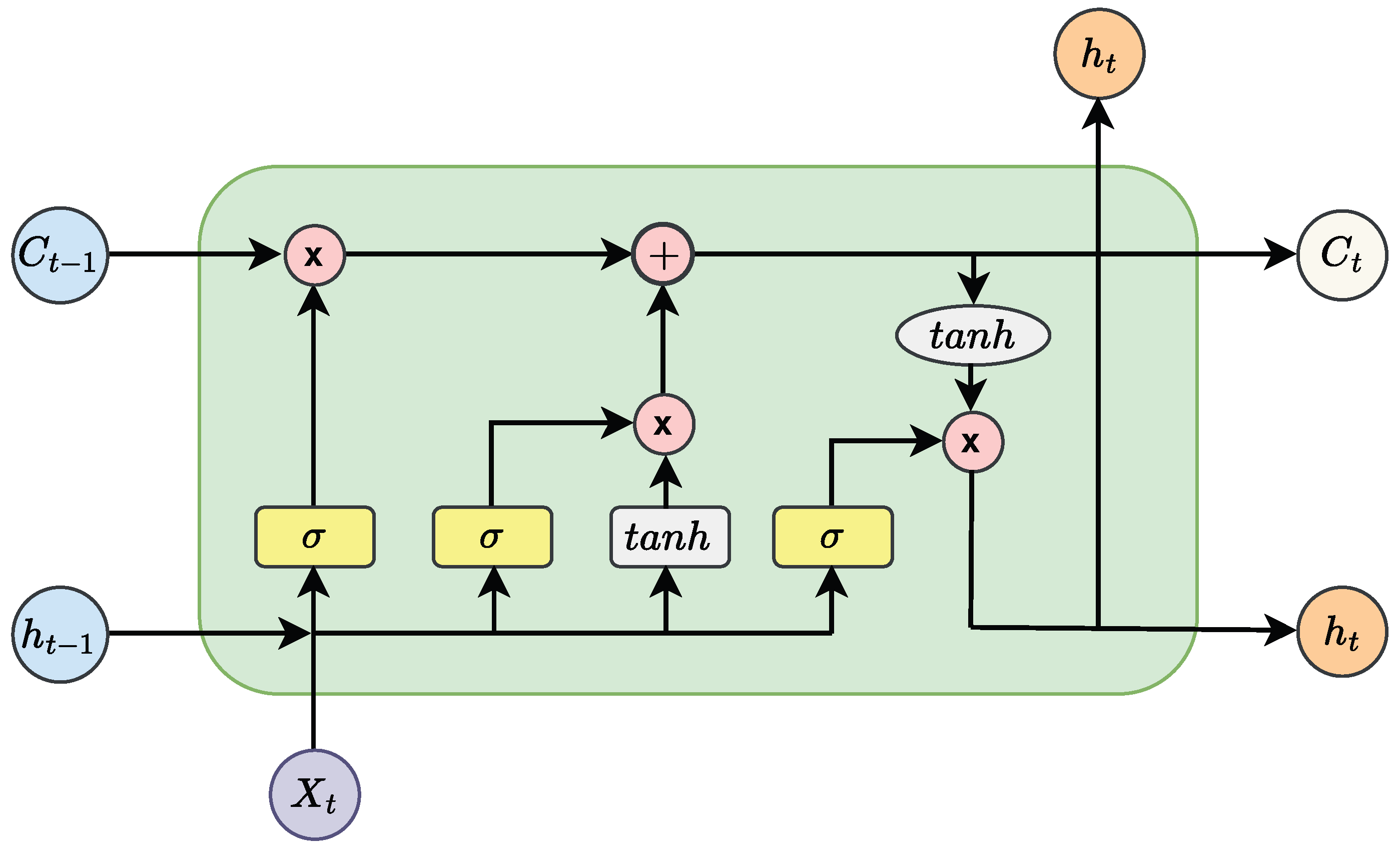
2.5.4. Long Short-Term Memory Neural Network (LSTM-NN)

Long Short-Term Memory (LSTM) is a type of Recurrent Neural Network (RNN) designed to address the vanishing gradient problem and to capture long-term dependencies in sequential data. A typical LSTM-NN is comprised of memory blocks called cells, where two states are being transferred to the next cell, the cell state and the hidden state. The construction process of an LSTM-NN is detailed in [31,32].

The general structure of the LSTM-NN can be observed in Figure 4.

2.5.5. Extreme Gradient Boosting (XGBoost)

XGBoost is a powerful and popular machine learning algorithm that belongs to the class of ensemble learning methods, specifically gradient boosting. XGBoost is widely used for both regression and classification tasks and has gained popularity due to its high performance and efficiency. XGBoost uses decision trees as base learners and combines them to form a strong learner. The principle of the XGBoost algorithm is explained in detail in [34,35].

The flow chart of the XGBoost algorithm is presented in Figure 5.

2.5.6. Light Gradient Boosting Machine (LightGBM)

LightGBM is an ensemble learning technique that utilizes a specialized form of decision trees called Gradient Boosted Decision Trees (GBDT). These trees are trained sequentially, where each subsequent tree corrects the mistakes made by the previous tree. LightGBM employs a leafwise tree growth strategy, which differs from the traditional levelwise strategy found in other gradient boosting frameworks like XGBoost [36]. The leafwise strategy tends to result in deeper trees and provides more accurate predictions [37].

LightGBM applies gradient-based optimization techniques to efficiently find the best split points and feature binning for each tree node. It uses a histogram-based approach to compute gradients for feature binning, which reduces memory usage and speeds up the computations [38].

2.6. Hyperparameter Tuning

Hyperparameters are parameters that are not directly learned from the data during model training, but are set prior to training and influence the learning process. Hyperparameter tuning involves searching for the optimal set of hyperparameters that maximize the performance of a model on a given task or dataset [39]. This process is essential for achieving the best possible model performance and generalization to unseen data.

Optuna is a popular open-source framework for hyperparameter optimization, developed by Akiba [40]. It provides an automated and efficient method for searching the best hyperparameters. This is accomplished by employing a technique known as “Sequential Model-Based Optimization” (SMBO), which iteratively explores the hyperparameter space and evaluates the performance of various configurations. It starts by sampling a set of hyperparameters from a predefined distribution and evaluates their performance using cross-validation or a validation set. Based on these evaluations, Optuna updates its internal method to focus the search on promising regions of the hyperparameter space [41].

In this paper, the Optuna framework was utilized for hyperparameter tuning of the RF, LSTM-NN, XGBoost, and LightGBM methods. The optimal hyperparameters found for each method with Optuna are as follows.

2.6.1. RF Hyperparameters

• Minimum samples leaf: 3;
• Number of estimators: 500;
• Minimum samples split: 7;
• Maximum depth: 30.

2.6.2. LSTM Hyperparameters

• Number of layers: 2;
• First layer: LSTM with 42 neurons and sigmoid activation function;
• Second layer: Dense with 16 neurons and ReLU activation function;
• Number of epochs: 10;
• Learning rate: 0.001.

2.6.3. XGBoost Hyperparameters

• Number of estimators: 500;
• Learning rate: 0.01;
• Minimum child weight: 1;
• Subsample: 0.7;
• Colsample by tree: 1;
• Regularization Alpha: 0;
• Regularization Lambda: 1;
• Objective: reg:linear;
• Booster: gbtree.

2.6.4. LightGBM Hyperparameters

• Number of leaves: 50;
• Learning rate: 0.1;
• Maximum depth: 5;
• Feature fraction: 0.9;
• Bagging fraction: 0.7;
• Bagging frequency: 10;
• Number of iterations: 50;
• Objective: regression.

2.7. Validation

This section includes the post-processing of the power consumption predictions obtained after the forecasting stage, the cross-validation process, and the performance evaluation of the forecasting methods based on statistical metrics and execution time.

2.7.1. Post-Processing

The following condition is verified:

$${\widehat{y}}_i\ge 0$$

(4)

We ensured the absence of negative power consumption predictions (${\widehat{y}}_i$). In case negative values of predicted power exist, those values are adjusted to 0.

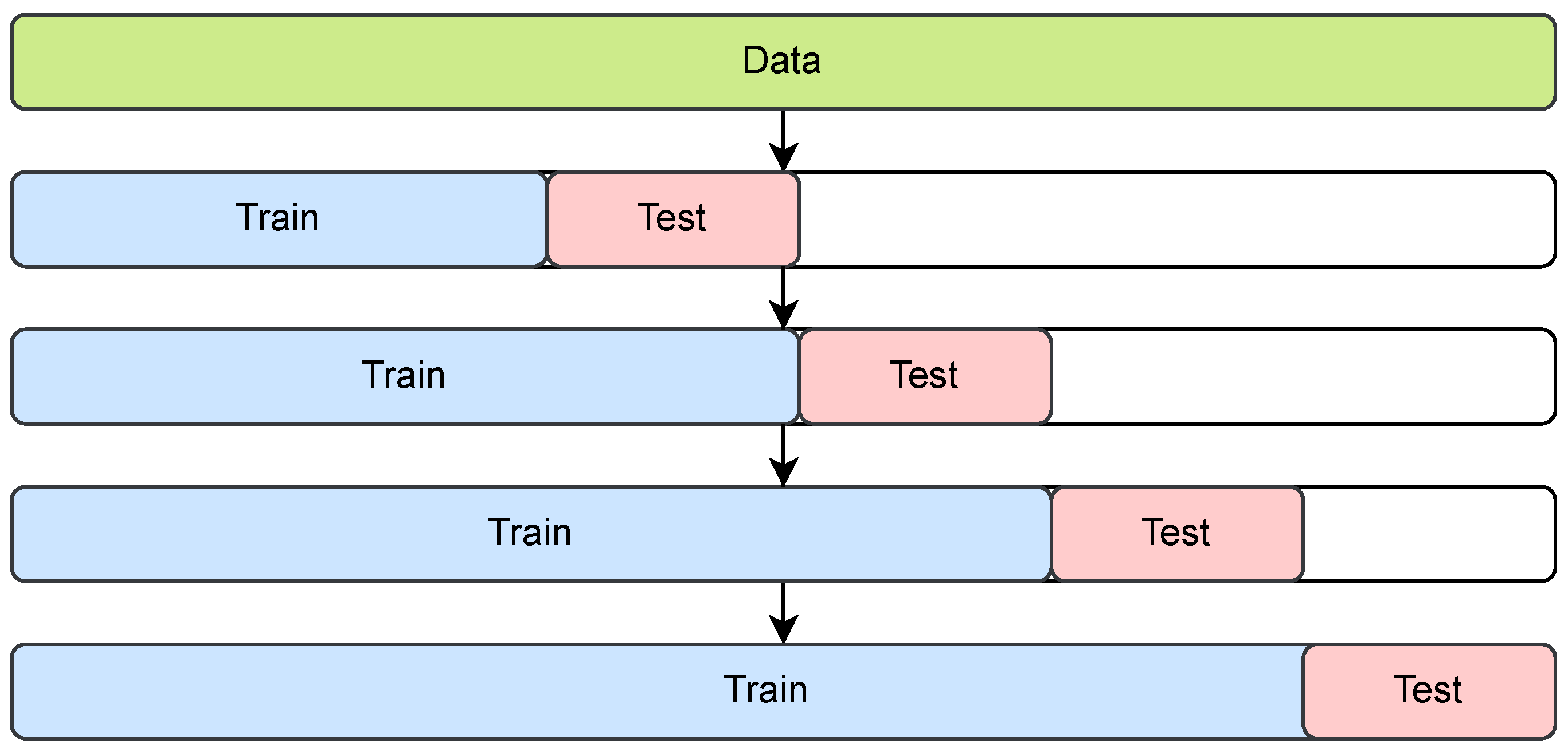
2.7.2. Cross-Validation

Cross-validation is a crucial technique in machine learning for assessing the performance and generalization ability of a model. The primary idea behind cross-validation is to split the dataset into multiple subsets, train the model on some of these subsets, and then, evaluate its performance on the remaining subsets [42]. This process helps provide a more robust estimate of the model’s performance compared to a single train–test split.

Time series split cross-validation is particularly suited for time series data. Unlike traditional k-fold cross-validation, and time series split maintains the temporal ordering of data when creating training and validation sets. This is crucial for time series data, where observations at a given time point may be dependent on previous time points.

For this reason, time series split cross-validation works on a rolling basis. It starts with a subset of data for training purposes, forecasts for the later data points, and then, checks the accuracy for the forecasted data points. Subsequently, the same forecasted data points are included as part of the next training dataset, and subsequent data points are forecasted. This process is repeated for the defined number of rounds. Figure 6 illustrates the time series split cross-validation process for four rounds.

2.7.3. Performance Evaluation

The F1-score, the Mean Absolute Error (MAE), the normalized root-mean-squared error (NRMSE), the coefficient of determination ($R^2$), and the model’s execution time were used to compare the performance of the forecasting methods. The F1-score metric was used for plugged-in status (classification), and the MAE, NRMSE, $R^2$, and execution time metrics were used for power consumption (regression):

• F1-score:

The F1-score is a metric commonly used in binary classification to evaluate the performance of a model. It combines two other metrics, precision and recall, into a single value [44]. These metrics are calculated using the concepts of true positives (TPs), false positives (FPs), and false negatives (FNs) as follows:

$$Precision=\frac{TP}{TP+FP}$$

(5)

$$Recall=\frac{TP}{TP+FN}$$

(6)

The F1-score is then calculated as the harmonic mean of the precision and recall:

$$F1=2\times \frac{Precision\times Recall}{Precision+Recall}$$

(7)

The F1-score ranges from 0 to 1, where 1 indicates perfect precision and recall and 0 indicates the worst possible performance. The harmonic mean gives more weight to lower values. This means that, for the F1-score to be high, both the precision and recall must be high, which is particularly useful when there is an uneven class distribution.

• Mean Absolute Error (MAE):

The MAE provides a measure of the average absolute deviation between the predicted and actual values. It represents the average magnitude of the errors in the same unit as the original data, making it easily interpretable [45]. A lower MAE indicates better accuracy, as it signifies that the model’s predictions are closer to the actual values. The MAE is defined as follows:

$$MAE=\frac{1}{n}\sum _{i=1}^n|y_i-{\widehat{y}}_i|$$

(8)

where $y_i$ is the real value, ${\widehat{y}}_i$ is the predicted value, and n is the sample size.

• Normalized root-mean-squared error (NRMSE)

The NRMSE is based on the root-mean-squared error (RMSE), which measures the square root of the average difference between predicted values and actual values, but normalized in this case by dividing by the maximum value of the actual value of power consumption. The resulting NRMSE value is expressed as a percentage, which is easy to interpret and allows for comparisons across different datasets. The NRMSE is defined as follows:

$$NRMSE(\%)=\frac{\sqrt{\frac{1}{n}{\sum }_{i=1}^n{(y_i-{\widehat{y}}_i)}^2}}{y_{max}-y_{min}}\times 100$$

(9)

where $y_i$ is the real value, ${\widehat{y}}_i$ is the predicted value, $y_{max}$ and $y_{min}$ are the maximum and minimum values of power consumption, and n is the sample size.

• Coefficient of determination ($R^2$):

The coefficient of determination, often denoted as the R-squared ($R^2$), is a statistical measure used to assess the goodness of fit of a regression model. It represents the proportion of the variance in the dependent variable that can be explained by the independent variables in the model. The R-squared ranges from 0 to 1 [46] and is defined as follows:

$$R^2=\left[\frac{{\sum }_{i=1}^n{(y_i-{\widehat{y}}_i)}^2}{{\sum }_{i=1}^n{(y_i-{\overline{y}}_i)}^2}\right]$$

(10)

where $y_i$ is the real value, ${\widehat{y}}_i$ is the predicted value, ${\overline{y}}_i$ is the mean of $y_i$, and n is the sample size.

• Execution time (in seconds):

The execution time refers to the duration it takes for the forecasting model to generate predictions or complete the forecasting process. It represents the computational effort required to implement the model and generate the desired output.

A faster execution time improves scalability and operational efficiency, particularly when dealing with real-time or high-frequency data [47]. Models with a faster execution time require fewer computational resources, including processing power and memory. Efficient resource utilization lowers the operational costs and improves overall system performance.

3. Case Study

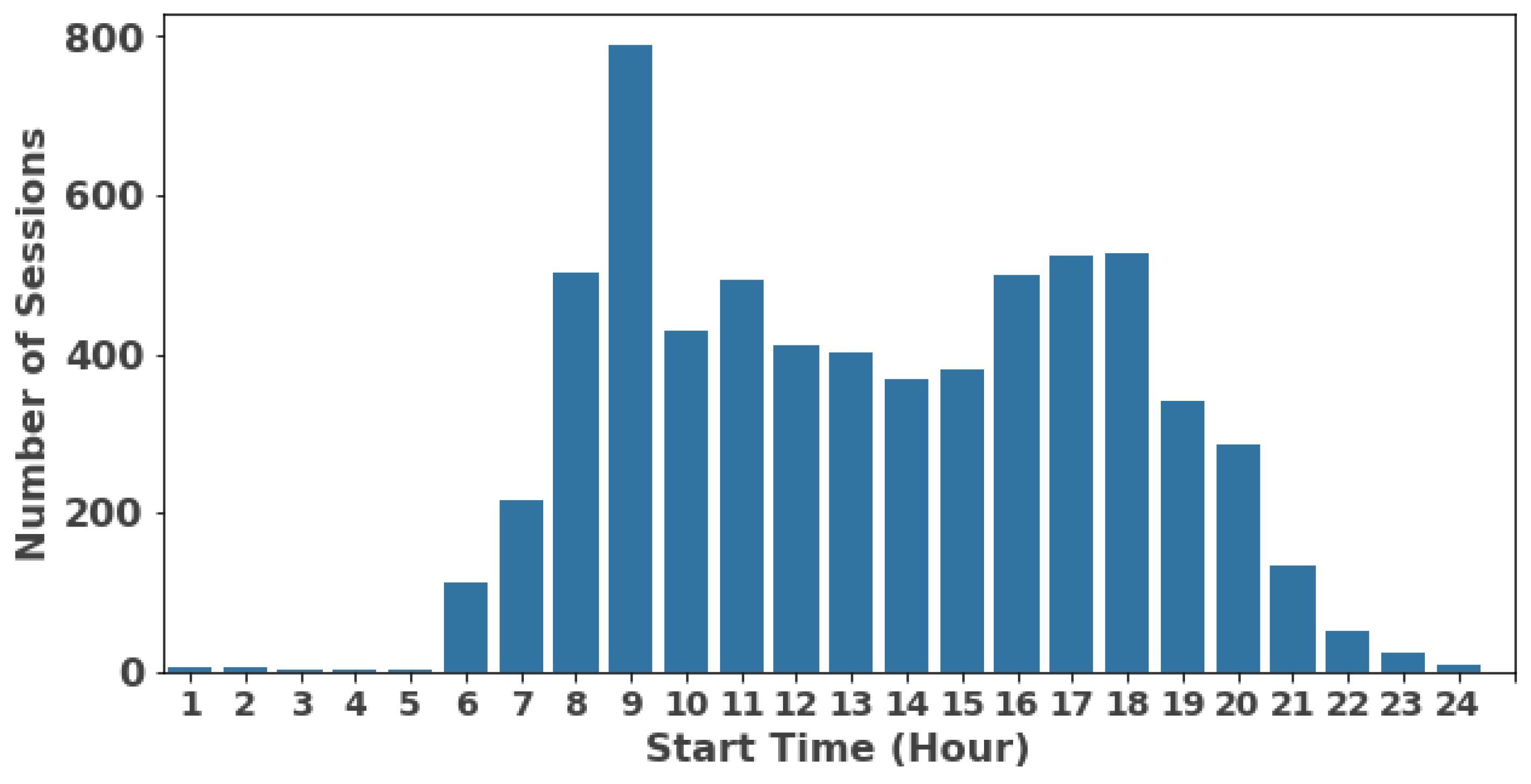
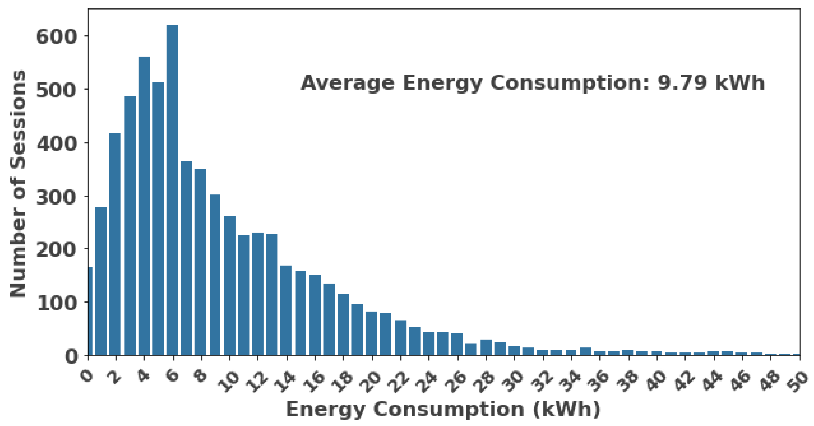
3.1. Data Description and Inputs

The dataset employed in this study pertains to the city of Boulder, Colorado, and is sourced from the City of Boulder Open Data Hub [48]. Given that the dataset includes all CSs within the city, this study hones in on the specific CS named “N BOULDER REC 1”. This particular CS contains 6508 EV charging session records spanning from August 2018 to May 2023. Each entry corresponds to an individual EV charging session, with provided data encompassing fields such as “Station Name”, “Address”, “start date time”, “end date time”, “Total Duration (hh:mm:ss)”, “charging duration (hh:mm:ss)”, “energy (kWh)”, “GHG Savings (kg)”, “Gasoline Savings (gallons)”, and “Port Type”.

The designated forecast horizon for this study spans a single day (day-ahead forecasting), with the forecast’s starting date set at “2023-05-04”. The choice of this forecasting day aims to optimally utilize the majority of the data available to train the models.

3.2. Pre-Processing

With the initial dataset of charging sessions, Figure 7, Figure 8 and Figure 9 were generated to illustrate the charging behavior at the CS. Figure 7 presents the distribution of the starting times (hours) for the charging sessions, revealing two distinct peaks, one occurring between 8 h and 9 h and another between 17 h and 18 h.

In Figure 8, the charging duration (measured in hours) of these sessions is depicted, with a majority lasting 1 h, although the average charging duration extends to 2 h.

Figure 9 presents the energy consumption pattern across charging sessions, indicating an average energy consumption of 9.79 kWh per charging session.

As outlined in Section 2.2, the initial dataset of the CS was transformed from charging sessions to a 15 min time series detailing plugged-in status and power consumption. Subsequently, missing values and outliers were addressed based on the approaches established.

Figure 10 depicts the logarithmic histogram of power consumption obtained. The distribution of the histogram appears to exhibit a bell-shaped curve with a peak around 3 kW, when excluding lower power consumption levels (between 0 and 0.3 kW), which represent the vast majority of the data. The extended tail on the right side of the histogram is indicative of occasional high-power consumption events, with a maximum power consumption of 6.6 kW.

3.3. Feature Engineering

Figure 11, Figure 12 and Figure 13 illustrate the power consumption behavior of EVs concerning several date/time features crafted during the feature engineering phase (Section 2.3).

Figure 11 presents the average power consumption per hour, offering insights into the daily CS pattern. Notably, two distinct peaks emerge: one at 9 h exhibiting an average power consumption of 2.2 kW and another at 16 h, with an average power consumption of 1.7 kW.

Figure 12 illustrates the average power consumption per month, revealing consistent trends across the entire year. All months exhibit a relatively uniform range of average power consumption, hovering between 1 kW and 1.3 kW. This suggests a consistent baseline of power demand at the CS, regardless of the specific month.

Figure 13 showcases the average power consumption distributed across the four seasons. Intriguingly, the values remain relatively close throughout the year, showcasing minimal variation. While slight fluctuations are observable, with the highest power consumption in spring and the lowest in fall, they are well within a narrow range, indicating that the impact of temperature and weather conditions is negligible at this CS.

Regarding the clustering process, Figure 14 was employed to define the optimal numbers of clusters (K) of power consumption. Based on the elbow method analysis, is was determined that the optimal number of clusters for this dataset is $K=5$. At this point, there is a noticeable change in the slope of the curve, and beyond this point, the reduction in the WCSS becomes less pronounced, indicating that additional clusters may not provide significant improvements in capturing the data variance.

Figure 15 shows the clusters (or groups) of power consumption obtained from the K-means method. Each data point in the plot corresponds to a specific power observation of the time series, while the color of the point indicates the cluster to which it belongs. By observing the plot, it becomes evident that the clustering algorithm effectively grouped data points with similar power consumption levels together. The mean power consumption values for each cluster are as follows: 0.01 kW for Cluster 1, 6.1 kW for Cluster 2, 3.1 kW for Cluster 3, 4.5 kW for Cluster 4, and 1.8 kW for Cluster 5.

3.3.1. Feature Selection

The Pearson correlation coefficients between power consumption and the other features in the dataset are presented in Figure 16. Features that exhibit a high positive correlation with power consumption are positioned towards the upper end of the matrix (in green), and features with a negative correlation are located towards the lower end (in yellow). Moreover, features with low correlation coefficients, suggesting little to no linear relationship with power consumption, are located in the middle of the matrix (in gray).

According to Figure 16, the most correlated features with power consumption are “cluster”, “Hour_x”, “Power lag 7”, “Power lag 5”, “Power lag 1”, and “Hour_y”.

Figure 17 shows the feature-selection results obtained using the filter method with the K best. The figure prioritizes and displays the best ten features correlated with power consumption, and the features are presented in descending order of their corresponding scores, indicating their significance. Based on the filter method results, the feature “Power lag 1” stands out as the most influential feature to predict the power consumption, followed by the other lag features and “cluster”.

Table 2. Most important features embedded method.

RF	XGBoost	LightGBM
Cluster	Power lag 7	Power lag 7
Day of year_y	Power lag 1	Power lag 5
Day of month_y	Power lag 5	Power lag 1
Power lag 1	Hour_x	Cluster
Power lag 7	Hour_y	Hour_y
Hour_x	Cluster	Hour_x
Power lag 5	Month_y	Day of year_x

provides a comprehensive overview of the seven most critical features to forecast the power consumption, obtained through the embedded method, specifically the feature importance technique, for the Random Forest, XGBoost, and LightGBM models. The features are listed from the most influential to the least influential, and notably, the best features identified for all three models correspond to the lag features, highlighting the importance of the temporal relationships in accurately predicting power usage patterns at the CS.

Based on the comprehensive examination of the results for feature selection, derived from the correlation matrix, filter method, and embedded method, a set of top features has emerged as the most influential predictors for accurate power consumption forecasting. These features include Power lag 1, Power lag 5, and Power lag 7, which capture historical consumption patterns and temporal dependencies. Additionally, the cluster feature, indicative of grouping power behaviors, and the Hour_x, Hour_y, Day of year_x, and Day of year_y attributes, representing the hour of the day and the day of the year, have demonstrated remarkable significance. These selected features collectively embody the interplay of temporal trends, historical patterns, and grouping behaviors, thereby forming a robust foundation for precise EV plugged-in status and power consumption forecasting at the CS.

To evaluate the impact of using different numbers of these eight top-ranked features on the performance of the machine learning models, an analysis using subsets of the highest-ranked features was conducted. The NRMSE for each model, using the top 2, 3, 4, 5, 6, 7, and 8 features, is summarized in

Table 3. NRMSE of the machine learning models using top-ranked features.

Model	NRMSE (%) Top Ranked Features
	Top 2	Top 3	Top 4	Top 5	Top 6	Top 7	Top 8
MLR	14.28	14.28	14.48	14.58	14.53	14.72	14.86
DT	4.32	4.50	4.31	4.18	4.80	4.25	4.37
RF	4.60	4.10	4.59	4.94	5.03	4.80	4.81
XGBoost	4.48	4.45	4.53	4.58	4.42	4.26	4.26
LightGBM	4.36	4.38	4.49	4.42	4.22	4.29	4.27
LSTM	9.92	9.90	10.01	10.20	9.40	9.87	9.91
Average	6.99	6.94	7.07	7.15	7.07	7.03	7.08

.

Table 3 shows that the differences in the NRMSE are minimal, indicating that the performance of the models is robust regardless of the number of top features used. These findings reinforce the validity of the feature-selection process and the reliability of the methods in capturing the essential patterns in the data.

3.3.2. Forecasting and Evaluation

Given that the forecasting day corresponds to 4 May 2023, the rest of the data were used for training, encompassing the time frame spanning from 22 August 2018 to 3 May 2023. In the forecasting phase, the first “plugged-in” variable is predicted every 15 min, to determine whether the EVs are connected or not, and subsequently, power consumption predictions are made for those 15 min intervals wherein EVs are connected.

Figure 18 presents the EVs’ charging behavior (plugged-in status and power consumption) for the forecasting day. The upper plot of Figure 18 displays the status of EVs being either plugged in (1) or unplugged (0) throughout the day. A clear pattern emerges, indicating a continuous connection of EVs from 8 h to 19 h, except for two brief periods: a 30 min interval from 12:30 h to 13 h and a 15 min interval from 17 h to 17:15 h, where no EVs are connected. The lower plot of Figure 18 focuses on the power consumption of EVs at the CS on the same day. There are five distinct “peaks” at various power consumption levels, but notably, the highest peak occurs at midday, for a 15 min interval from 11:45 h to 12 h, revealing a high power consumption of 6.42 kW at the CS.

As mentioned in Section 2.5, the XGBoost classifier was employed to forecast the plugged-in status. This predictive model aimed to determine whether an EV is connected (1) or not (0) throughout the forecasting day. The results obtained from the binary classification model are visually depicted through the confusion matrix in Figure 19.

The confusion matrix illustrates the model’s ability to correctly classify the 96 instances (intervals) of the forecasting day into four categories:

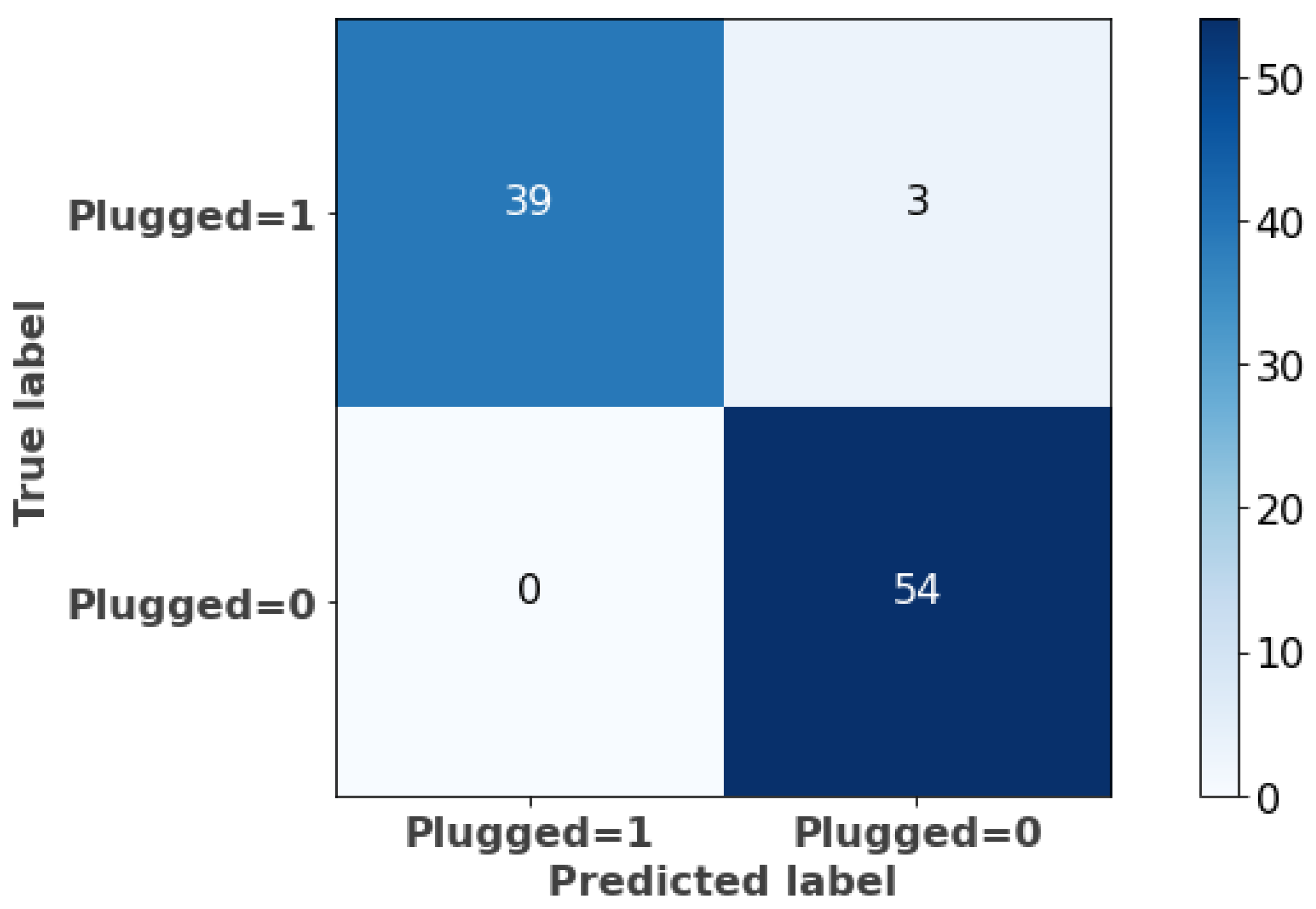
• True positives (TPs): There are 39 instances where the actual class was plugged-in (1) and the model has correctly predicted them as plugged-in (1).
• False positives (FPs): The model has predicted three instances as unplugged (0), when the actual class was plugged (1).
• False negatives (FNs): The model did not predict any instances as plugged-in (1), when the actual class was unplugged (0).
• True negatives (TNs): The model has correctly predicted 54 instances as unplugged (0), when the actual class was unplugged (0).

It is evident that the model performs well in terms of true positives and true negatives. It correctly identifies positive cases (TPs = 39) and true negative cases (TNs = 54), and the small number of false positives (FPs = 3) suggests that the model occasionally misclassifies negative instances as positive. Overall, the forecasting model for plugged-in status presents an F1-score of 0.97.

To forecast the power consumption, the six regression methods mentioned and explained in Section 2.5 were tested using the hyperparameters found in Section 2.6. The results obtained are summarized in

Table 4. Comparative performance for all methods.

Model	Performance Evaluation
	NRMSE (%)	MAE (kW)	${\mathit{R}}^{\mathbf{2}}$	Execution Time (s)
LightGBM	4.22	0.15	0.97	5.0
XGBoost	4.42	0.15	0.97	50.0
DT	4.80	0.16	0.96	0.5
RF	5.03	0.16	0.96	180.0
LSTM-NN	9.40	0.25	0.86	780.0
MLR	14.53	0.59	0.58	0.2

, which compares the performance of each method in terms of the evaluation metrics and the model’s execution time.

The results presented in Table 4 indicate that the methods based on gradient boosting, namely LightGBM and XGBoost, outperformed the rest of the methods. LightGBM achieved a lower NRMSE, with an error of 4.22%, while for XGBoost, the NRMSE was 4.42%. Both methods, with an $R^2$ of 0.97, exhibit highly comparable performance metrics, showcasing their effectiveness in EV power consumption prediction accuracy. However, when comparing the execution times, LightGBM emerges as the more efficient option, with computations taking 5 s, being ten-times faster than XGBoost.

DT and RF also performed well, having similar values of the NRMSE, 4.80% and 5.03%, respectively, and the same $R^2$ of 0.96. Nevertheless, DT stands out for its remarkable computational efficiency, completing the computations within just half a second. RF, on the other hand, requires significantly more time, with computations taking 180 s due to its ensemble nature and the complexity associated with aggregating multiple decision trees.

The LSTM-NN, while renowned for its capacity to capture complex temporal patterns, presents certain limitations within this context when compared to the other methods. The higher NRMSE value of 9.40% and an $R^2$ of 0.86 suggest that LSTM-NN’s predictions exhibit more variability, and the longer execution time of 780 s is a disadvantage. MLR (the simplest method used for benchmarking) displays the lowest accuracy among all the methods, as evidenced by a higher NRMSE of 14.53% and an $R^2$ of 0.58.

Additionally, Figure 20 shows the actual power consumption and the corresponding predictions derived from each method. The blue line represents the real power consumed at the CS in that day, and the red, purple, gray, yellow, orange, and green dashed lines represent the power consumption predictions for MLR, DT, RF, XGBoost, LightGBM, and the LSTM-NN, respectively.

After comparing the six regression methods, LightGBM appeared as the most effective (best overall performance) for predicting the power consumption of EVs at the CS. The differences in the predictions among all forecasting methods were small, with the exception of the MLR method, which is used as a benchmark for the rest of the methods. In general, the power consumption forecasting results were very similar to the trend of real power consumption, which explains the very good model performances obtained.

Figure 21 compares in detail the real vs. the predicted plugged-in status (upper plot) and power consumption (lower plot) for the forecasting day. The actual plugged-in status and power consumption values correspond to the blue lines, and the predicted plugged-in status (XGBoost classifier results) and power consumption (LightGBM) corresponds to the orange dashed lines.

The upper plot of Figure 21 attests to the effectiveness of the forecasting model in accurately predicting EVs’ plugged-in status. The majority of the day demonstrates a remarkable alignment between the actual and predicted behaviors, with the model effectively capturing the nuances of EVs’ charging patterns. A few deviations can be observed between the actual and predicted plugged-in status, around 13:30 h to 14:30 h, where the model anticipated an intermittent unplugging, contrary to the continuous plugged-in state observed. These discrepancies, while limited in occurrence, underscore the challenge of capturing transient behaviors and unexpected shifts in EVs’ charging activity.

In the lower plot of Figure 21, it is evident that, for the most part, the predicted and actual EVs’ power consumption closely align. The forecasting model successfully captures the overall trend and magnitude of EVs’ power usage, depicting periods of power consumption and idle intervals. Notably, the model predicted the highest power consumption peak around 11:30 h, with a slight difference, but overestimated the actual power consumption from 13 h to 14 h, predicting around 1.85 kW, while the actual consumption was 1.05 kW. Similarly, from 17 h to 19 h, the model underestimated the power consumption, leading to a discrepancy between the predicted and actual values.

In essence, the forecasting model’s strengths lie in its ability to predict overarching trends in EVs’ charging behavior, namely plugged-in status and power consumption, accurately. These strengths equip energy stakeholders with valuable information to optimize resource allocation, manage peak loads, enhance grid stability, and support sustainable energy practices.

3.3.3. Cross-Validation

A time series split cross-validation was performed as outlined in Section 2.7.2, to assess and validate the accuracy obtained by the LightGBM method. A fixed test size of 96 points (1 day) was defined using five rounds, which means that the 5 days prior to the forecasting day were also forecasted, 1 day in each round.

Figure 22 compares the power consumption forecasts obtained in the cross-validation for the 5 days prior to “2023-05-04” and the actual values.

The results in Figure 22 are consistent with the results obtained for the forecasting day. Furthermore, the NRMSE obtained for the cross-validation was 5.21%, slightly higher than the NRMSE of 4.22% observed for the forecasting day. This marginal rise in error can be expected in cross-validated scenarios, as the model is rigorously tested on diverse subsets of the data, reinforcing its ability to maintain consistency in predicting power consumption trends over varying time frames. The results underscore the model’s reliability and suggest that its forecasting capabilities extend beyond isolated predictions, thereby enhancing its applicability and credibility.

4. Conclusions and Limitations

4.1. Main Conclusions

EV charging behavior is highly dynamic and variable, influenced by factors such as the discrete behavior going from 0 to Pmax when the EVs start charging, the type of EV, the battery capacity, the charging speed, user habits, and the time of day. This variability can lead to significant differences in charging patterns, as daily commutes, access to charging infrastructure, and individual preferences play crucial roles.

In line with these unique characteristics, a methodological framework for accurate EV charging behavior forecasting at CSs has been proposed in this paper. The structured and robust framework is able to transform EVs’ charging sessions data into a 15 min plugged-in status and power consumption time series during the pre-processing and to apply the stages of feature engineering, feature selection, forecasting methods, and validation.

The proposed framework has been applied on a real-world dataset from Boulder city, and the results demonstrated the effectiveness of the framework in the task of EVs’ plugged-in status and power consumption forecasting at CSs. XGBoost’s classifier predicted EVs’ plugging-in status with remarkable accuracy, setting the stage for precise power consumption forecasting. A comprehensive evaluation of six regression methods spotlighted the supremacy of gradient boosting algorithms, with LightGBM emerging as the the most effective method to forecast EVs’ power consumption, due to its optimal balance between performance and computational efficiency.

The insights gained from this study have profound implications for power grid management and the seamless integration of EVs. As EVs transition from being a passive consumer to an active participant in the grid, this framework equips power system operators with a strategic advantage in anticipating and adapting to the evolving landscape. Moreover, the proposed framework can be applied to any scale of CS, with the assumption that EVs’ charging sessions are known and the inputs are established.

4.2. Limitations

While this study has made significant strides in accurately forecasting electric vehicles’ (EVs) charging behavior at charging stations (CSs), several inherent limitations warrant consideration. The dataset used in this study was recorded at specific time intervals, which may not capture rapid fluctuations or finer details in EV charging patterns. Higher resolution data, with more frequent sampling intervals, could provide a more detailed and accurate representation of EV charging behavior.

The forecasting models developed in this study rely heavily on historical data. While historical data provide valuable insights, they may not fully capture evolving patterns due to unforeseen changes in EV technology, user behaviors, or external factors such as policy changes and economic shifts. This reliance may limit the models’ ability to adapt to future changes and emerging trends in EV usage.

The computational complexity and efficiency of the models were appropriate for the given dataset size and forecasting requirements. However, scalability and real-time forecasting in large-scale datasets may pose additional challenges. Computational limitations could affect the feasibility of applying the proposed models in real time or on larger datasets without optimization and resource allocation.

To enhance the framework’s versatility and robustness, future research endeavors could focus on expanding its scope to encompass diverse geographical locations, varied charging behaviors, and the integration of other relevant variables. This would require further validation and adaptation of the methodology to accommodate different contexts and datasets.

References

1. IEA. Global EV Outlook 2023: Catching Up with Climate Ambitions; International Energy Agency: Paris, France, 2023; pp. 1–142. [Google Scholar]
2. Fit for 55: MEPs Back Objective of Zero Emissions for Cars and Vans in 2035 | News | European Parliament, 2022. Available online: https://www.europarl.europa.eu/news/en/press-room/20220603IPR32129/fit-for-55-meps-back-objective-of-zero-emissions-for-cars-and-vans-in-2035 (accessed on 7 May 2024).
3. Deliverable D1.1 Electric Road Mobility Evolution Scenarios. Available online: https://cordis.europa.eu/project/id/101056765 (accessed on 12 March 2024).
4. Guzman, C.P.; Bañol Arias, N.; Franco, J.F.; Rider, M.J.; Romero, R. Enhanced coordination strategy for an aggregator of distributed energy resources participating in the day-ahead reserve market. Energies 2020, 13, 1965. [Google Scholar] [CrossRef]
5. Zhu, J.; Yang, Z.; Mourshed, M.; Guo, Y.; Zhou, Y.; Chang, Y.; Wei, Y.; Feng, S. Electric vehicle charging load forecasting: A comparative study of deep learning approaches. Energies 2019, 12, 2692. [Google Scholar] [CrossRef]
6. Sousa, T.; Soares, T.; Morais, H.; Castro, R.; Vale, Z. Simulated annealing to handle energy and ancillary services joint management considering electric vehicles. Electr. Power Syst. Res. 2016, 136, 383–397. [Google Scholar] [CrossRef]
7. Shahriar, S.; Al-Ali, A.R.; Osman, A.H.; Dhou, S.; Nijim, M. Machine learning approaches for EV charging behavior: A review. IEEE Access 2020, 8, 168980–168993. [Google Scholar] [CrossRef]
8. Abbas, F.; Feng, D.; Habib, S.; Rasool, A.; Numan, M. An improved optimal forecasting algorithm for comprehensive electric vehicle charging allocation. Energy Technol. 2019, 7, 1900436. [Google Scholar] [CrossRef]
9. Jia, Z.; Li, J.; Zhang, X.P.; Zhang, R. Review on Optimization of Forecasting and Coordination Strategies for Electric Vehicle Charging. J. Mod. Power Syst. Clean Energy 2022, 11, 389–400. [Google Scholar] [CrossRef]
10. Xing, Y.; Li, F.; Sun, K.; Wang, D.; Chen, T.; Zhang, Z. Multi-type electric vehicle load prediction based on Monte Carlo simulation. Energy Rep. 2022, 8, 966–972. [Google Scholar] [CrossRef]
11. Ullah, I.; Liu, K.; Yamamoto, T.; Al Mamlook, R.E.; Jamal, A. A comparative performance of machine learning algorithm to predict electric vehicles energy consumption: A path towards sustainability. Energy Environ. 2022, 33, 1583–1612. [Google Scholar] [CrossRef]
12. Zheng, Y.; Shao, Z.; Zhang, Y.; Jian, L. A systematic methodology for mid-and-long term electric vehicle charging load forecasting: The case study of Shenzhen, China. Sustain. Cities Soc. 2020, 56, 102084. [Google Scholar] [CrossRef]
13. Lu, Y.; Li, Y.; Xie, D.; Wei, E.; Bao, X.; Chen, H.; Zhong, X. The application of improved random forest algorithm on the prediction of electric vehicle charging load. Energies 2018, 11, 3207. [Google Scholar] [CrossRef]
14. Gruosso, G.; Mion, A.; Gajani, G.S. Forecasting of electrical vehicle impact on infrastructure: Markov chains model of charging stations occupation. ETransportation 2020, 6, 100083. [Google Scholar] [CrossRef]
15. Douaidi, L.; Senouci, S.M.; El Korbi, I.; Harrou, F. Predicting Electric Vehicle Charging Stations Occupancy: A Federated Deep Learning Framework. In Proceedings of the 2023 IEEE 97th Vehicular Technology Conference (VTC2023-Spring), Florence, Italy, 20–23 June 2023; pp. 1–5. [Google Scholar]
16. Shahriar, S.; Al-Ali, A.R.; Osman, A.H.; Dhou, S.; Nijim, M. Prediction of EV charging behavior using machine learning. IEEE Access 2021, 9, 111576–111586. [Google Scholar] [CrossRef]
17. Jeon, Y.E.; Kang, S.B.; Seo, J.I. Hybrid Predictive Modeling for Charging Demand Prediction of Electric Vehicles. Sustainability 2022, 14, 5426. [Google Scholar] [CrossRef]
18. Kim, T.; Ko, W.; Kim, J. Analysis and impact evaluation of missing data imputation in day-ahead PV generation forecasting. Appl. Sci. 2019, 9, 204. [Google Scholar] [CrossRef]
19. Ikotun, A.M.; Ezugwu, A.E.; Abualigah, L.; Abuhaija, B.; Heming, J. K-means clustering algorithms: A comprehensive review, variants analysis, and advances in the era of big data. Inf. Sci. 2023, 622, 178–210. [Google Scholar] [CrossRef]
20. Sinaga, K.P.; Yang, M.S. Unsupervised K-means clustering algorithm. IEEE Access 2020, 8, 80716–80727. [Google Scholar] [CrossRef]
21. Ghosh, J.; Liu, A. K-means. The Top Ten Algorithms in Data Mining; CRC Press: Boca Raton, FL, USA, 2009; pp. 21–35. [Google Scholar]
22. Cui, M. Introduction to the k-means clustering algorithm based on the elbow method. Account. Audit. Financ. 2020, 1, 5–8. [Google Scholar] [CrossRef]
23. Ganti, A. Correlation coefficient. Corp. Financ. Acc. 2020, 9, 145–152. [Google Scholar]
24. Khalid, N.H.M.; Ismail, A.R.; Aziz, N.A.; Hussin, A.A.A. Performance Comparison of Feature Selection Methods for Prediction in Medical Data. In Proceedings of the International Conference on Soft Computing in Data Science, Online, 24–25 January 2023; pp. 92–106. [Google Scholar]
25. Zheng, H.; Yuan, J.; Chen, L. Short-term load forecasting using EMD-LSTM neural networks with a Xgboost algorithm for feature importance evaluation. Energies 2017, 10, 1168. [Google Scholar] [CrossRef]
26. Maulud, D.; Abdulazeez, A.M. A review on linear regression comprehensive in machine learning. J. Appl. Sci. Technol. Trends 2020, 1, 140–147. [Google Scholar] [CrossRef]
27. Costa, V.G.; Pedreira, C.E. Recent advances in decision trees: An updated survey. Artif. Intell. Rev. 2023, 56, 4765–4800. [Google Scholar] [CrossRef]
28. Antoniadis, A.; Lambert-Lacroix, S.; Poggi, J.M. Random forests for global sensitivity analysis: A selective review. Reliab. Eng. Syst. Saf. 2021, 206, 107312. [Google Scholar] [CrossRef]
29. Afzal, A.; Aabid, A.; Khan, A.; Khan, S.A.; Rajak, U.; Verma, T.N.; Kumar, R. Response surface analysis, clustering, and random forest regression of pressure in suddenly expanded high-speed aerodynamic flows. Aerosp. Sci. Technol. 2020, 107, 106318. [Google Scholar] [CrossRef]
30. Singh, U.; Rizwan, M.; Alaraj, M.; Alsaidan, I. A machine learning-based gradient boosting regression approach for wind power production forecasting: A step towards smart grid environments. Energies 2021, 14, 5196. [Google Scholar] [CrossRef]
31. Le, X.H.; Ho, H.V.; Lee, G.; Jung, S. Application of Long Short-Term Memory (LSTM) Neural Network for Flood Forecasting. Water 2019, 11, 1387. [Google Scholar] [CrossRef]
32. Staudemeyer, R.C.; Morris, E.R. Understanding LSTM–a tutorial into long short-term memory recurrent neural networks. arXiv 2019, arXiv:1909.09586. [Google Scholar]
33. Essam, Y.; Ahmed, A.N.; Ramli, R.; Chau, K.W.; Idris Ibrahim, M.S.; Sherif, M.; Sefelnasr, A.; El-Shafie, A. Investigating photovoltaic solar power output forecasting using machine learning algorithms. Eng. Appl. Comput. Fluid Mech. 2022, 16, 2002–2034. [Google Scholar] [CrossRef]
34. Liu, J.J.; Liu, J.C. Permeability predictions for tight sandstone reservoir using explainable machine learning and particle swarm optimization. Geofluids 2022, 2022, 2263329. [Google Scholar] [CrossRef]
35. Torres-Barrán, A.; Alonso, Á.; Dorronsoro, J.R. Regression tree ensembles for wind energy and solar radiation prediction. Neurocomputing 2019, 326, 151–160. [Google Scholar] [CrossRef]
36. Shehadeh, A.; Alshboul, O.; Al Mamlook, R.E.; Hamedat, O. Machine learning models for predicting the residual value of heavy construction equipment: An evaluation of modified decision tree, LightGBM, and XGBoost regression. Autom. Constr. 2021, 129, 103827. [Google Scholar] [CrossRef]
37. Al Daoud, E. Comparison between XGBoost, LightGBM and CatBoost using a home credit dataset. Int. J. Comput. Inf. Eng. 2019, 13, 6–10. [Google Scholar]
38. Guo, J.; Yun, S.; Meng, Y.; He, N.; Ye, D.; Zhao, Z.; Jia, L.; Yang, L. Prediction of heating and cooling loads based on light gradient boosting machine algorithms. Build. Environ. 2023, 236, 110252. [Google Scholar] [CrossRef]
39. Weerts, H.J.; Mueller, A.C.; Vanschoren, J. Importance of tuning hyperparameters of machine learning algorithms. arXiv 2020, arXiv:2007.07588. [Google Scholar]
40. Akiba, T.; Sano, S.; Yanase, T.; Ohta, T.; Koyama, M. Optuna: A next-generation hyperparameter optimization framework. In Proceedings of the 25th ACM SIGKDD International Conference on Knowledge Discovery & Data Mining, Anchorage, AK, USA, 4–8 August 2019; pp. 2623–2631. [Google Scholar]
41. Srinivas, P.; Katarya, R. hyOPTXg: OPTUNA hyper-parameter optimization framework for predicting cardiovascular disease using XGBoost. Biomed. Signal Process. Control 2022, 73, 103456. [Google Scholar] [CrossRef]
42. Bergmeir, C.; Benítez, J.M. On the use of cross-validation for time series predictor evaluation. Inf. Sci. 2012, 191, 192–213. [Google Scholar] [CrossRef]
43. Shrivastava, S. Cross Validation in Time Series, 2020. Available online: https://medium.com/@soumyachess1496/cross-validation-in-time-series-566ae4981ce4 (accessed on 7 May 2024).
44. Mehdiyev, N.; Enke, D.; Fettke, P.; Loos, P. Evaluating forecasting methods by considering different accuracy measures. Procedia Comput. Sci. 2016, 95, 264–271. [Google Scholar] [CrossRef]
45. Hyndman, R.J.; Koehler, A.B. Another look at measures of forecast accuracy. Int. J. Forecast. 2006, 22, 679–688. [Google Scholar] [CrossRef]
46. Lateko, A.A.H.; Yang, H.T.; Huang, C.M. Short-Term PV Power Forecasting Using a Regression-Based Ensemble Method. Energies 2022, 15, 4171. [Google Scholar] [CrossRef]
47. Zainab, A.; Syed, D.; Ghrayeb, A.; Abu-Rub, H.; Refaat, S.S.; Houchati, M.; Bouhali, O.; Bañales Lopez, S. A Multiprocessing-Based Sensitivity Analysis of Machine Learning Algorithms for Load Forecasting of Electric Power Distribution System. IEEE Access 2021, 9, 31684–31694. [Google Scholar] [CrossRef]
48. City of Colorado. Electric Vehicle Charging Station Energy Consumption in the City of Boulder, Colorado, 2023. Available online: https://bouldercolorado.gov/services/electric-vehicle-charging-stations (accessed on 7 May 2024).
Figure 1. Proposed forecasting methodology.
Energies 17 03396 g001
Figure 2. DT structure.
Energies 17 03396 g002
Figure 3. RF structure.
Energies 17 03396 g003
Figure 4. LSTM structure (based on [33]).
Energies 17 03396 g004
Figure 5. Flow chart of XGBoost (based on [34]).
Energies 17 03396 g005
Figure 6. Time series split cross validation: 4 rounds (based on [43]).
Energies 17 03396 g006
Figure 7. EVs charging start time.
Energies 17 03396 g007
Figure 8. EVs’ charging duration.
Energies 17 03396 g008
Figure 9. EVs’ energy consumption.
Energies 17 03396 g009
Figure 10. EVs power consumption histogram.
Energies 17 03396 g010
Figure 11. Average power consumption per hour.
Energies 17 03396 g011
Figure 12. Average power consumption per month.
Energies 17 03396 g012
Figure 13. Average power consumption per season.
Energies 17 03396 g013
Figure 14. Optimal number of clusters elbow method.
Energies 17 03396 g014
Figure 15. Power consumption clusters.
Energies 17 03396 g015
Figure 16. Correlation matrix for power consumption.
Energies 17 03396 g016
Figure 17. Feature-selection filter method.
Energies 17 03396 g017
Figure 18. Plugged-in status and power consumption for forecasting day.
Energies 17 03396 g018
Figure 19. Confusion matrix for plugged-in status.
Energies 17 03396 g019
Figure 20. Power consumption forecast results.
Energies 17 03396 g020
Figure 21. Real vs. predicted plugged-in status and power consumption.
Energies 17 03396 g021
Figure 22. Power consumption forecast cross-validation.
Energies 17 03396 g022