
Price Risk Exposure of Small Participants in Liberalized Multi-National Power Markets: A Case Study on the Belize–Mexico Interconnection


Abstract
:1. Introduction
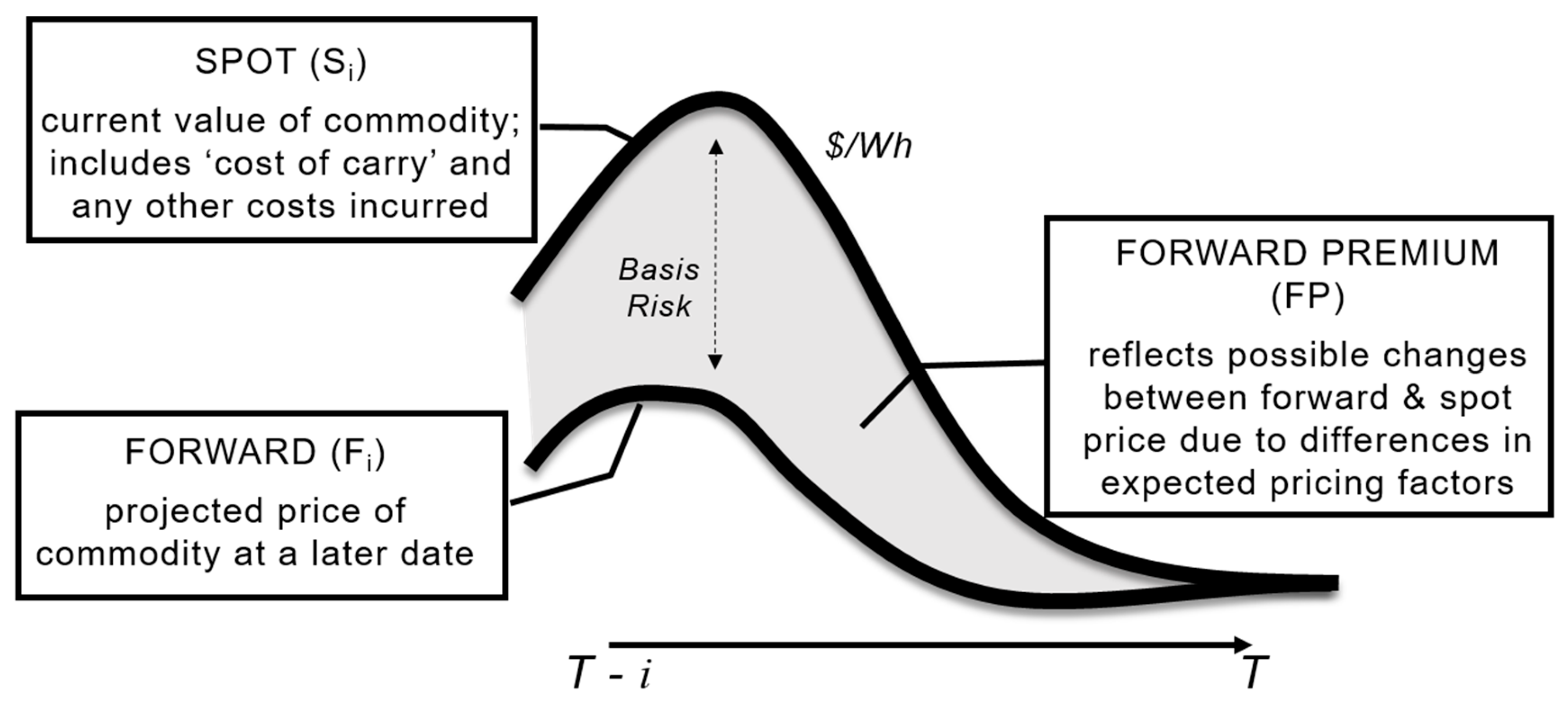
2. Background
2.1. Empirical Analysis of Electricity Forward and Spot Pricing
2.2. Study Aim and Structure
3. Materials and Methods
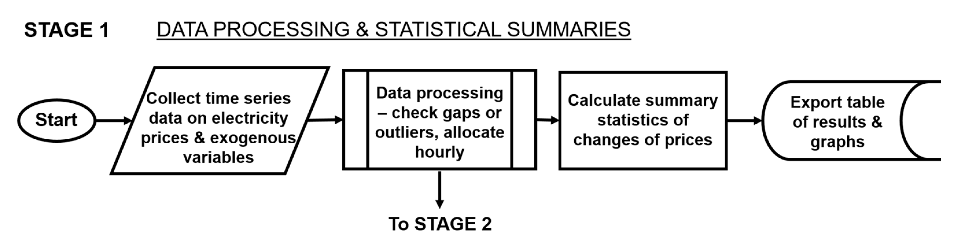
3.1. Study Design
3.2. The Data
3.3. Data Analysis
4. Discussion of Results
4.1. Data Analysis of Forward and Spot Market Conditions
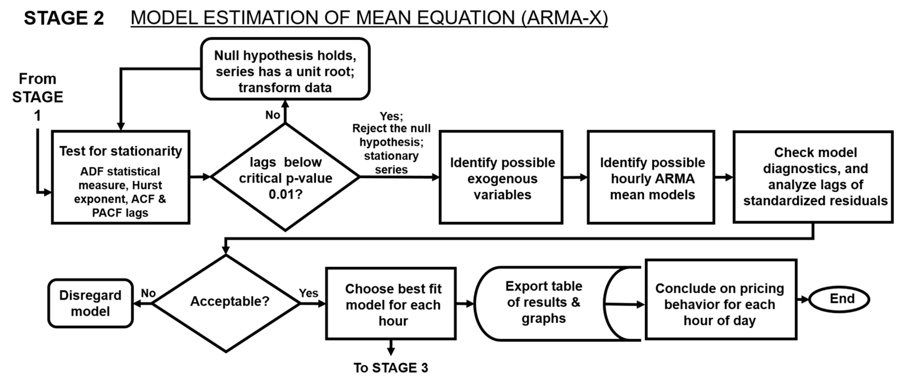
4.2. Time-Series Analysis for Determining Conditional Mean Equations for Pricing Series
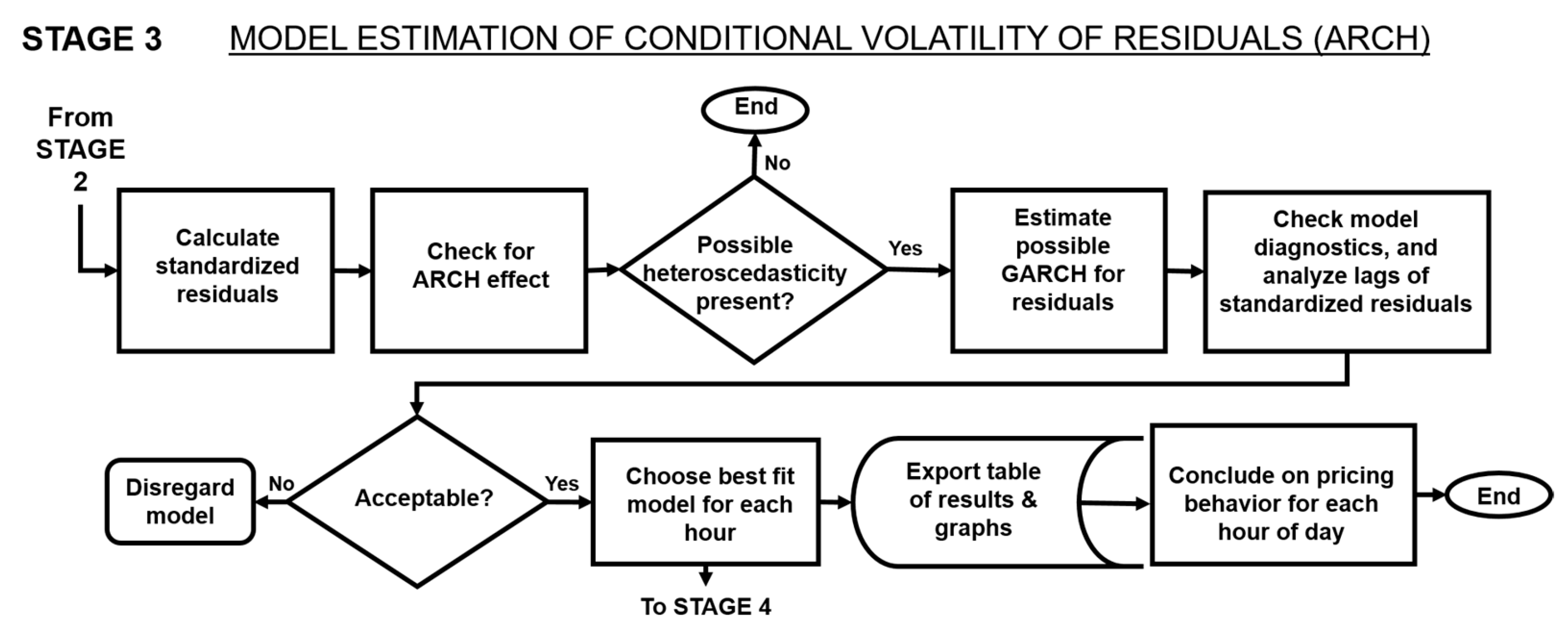
4.3. Modeling the Volatility of Residuals as a Risk Measure for Pricing Series
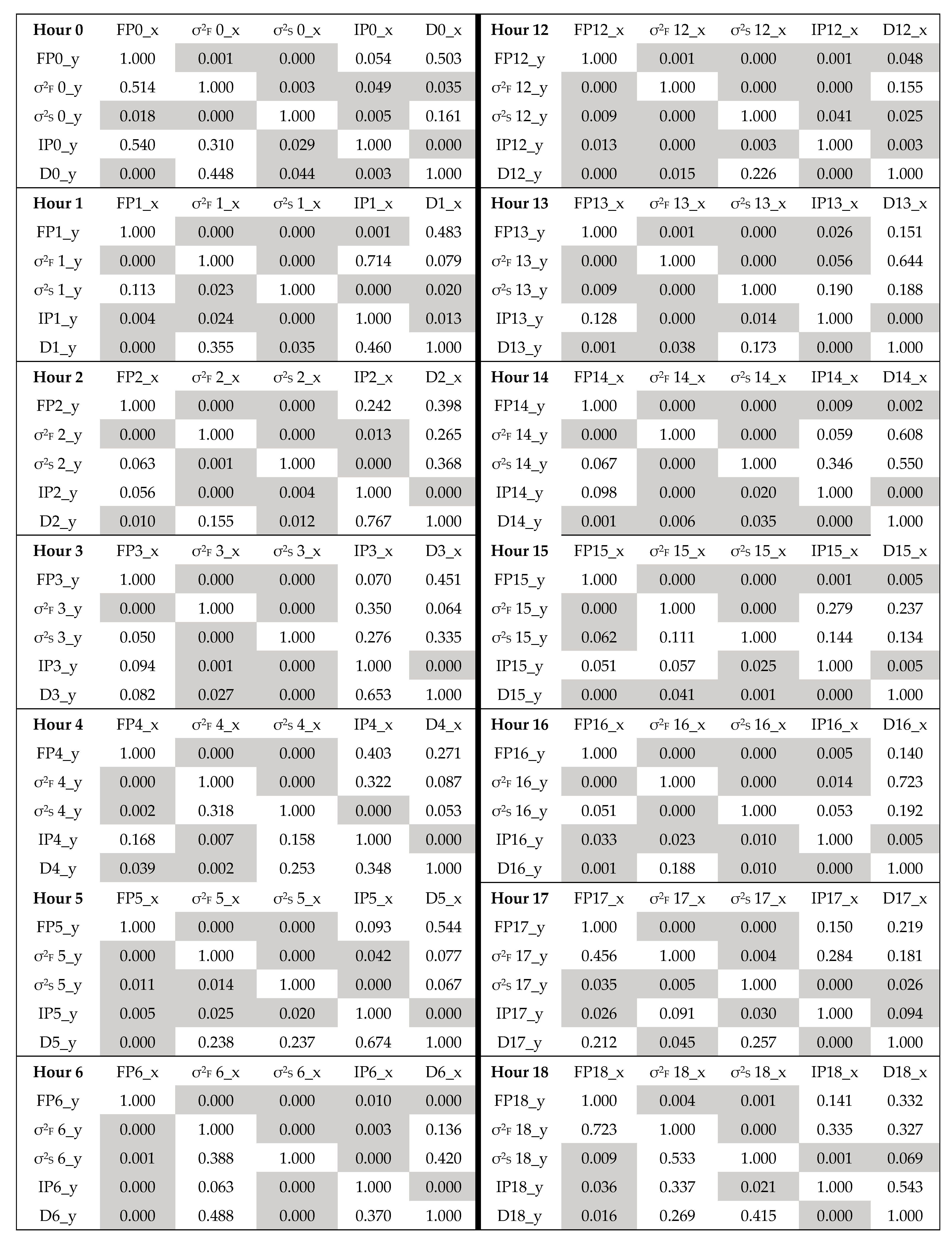
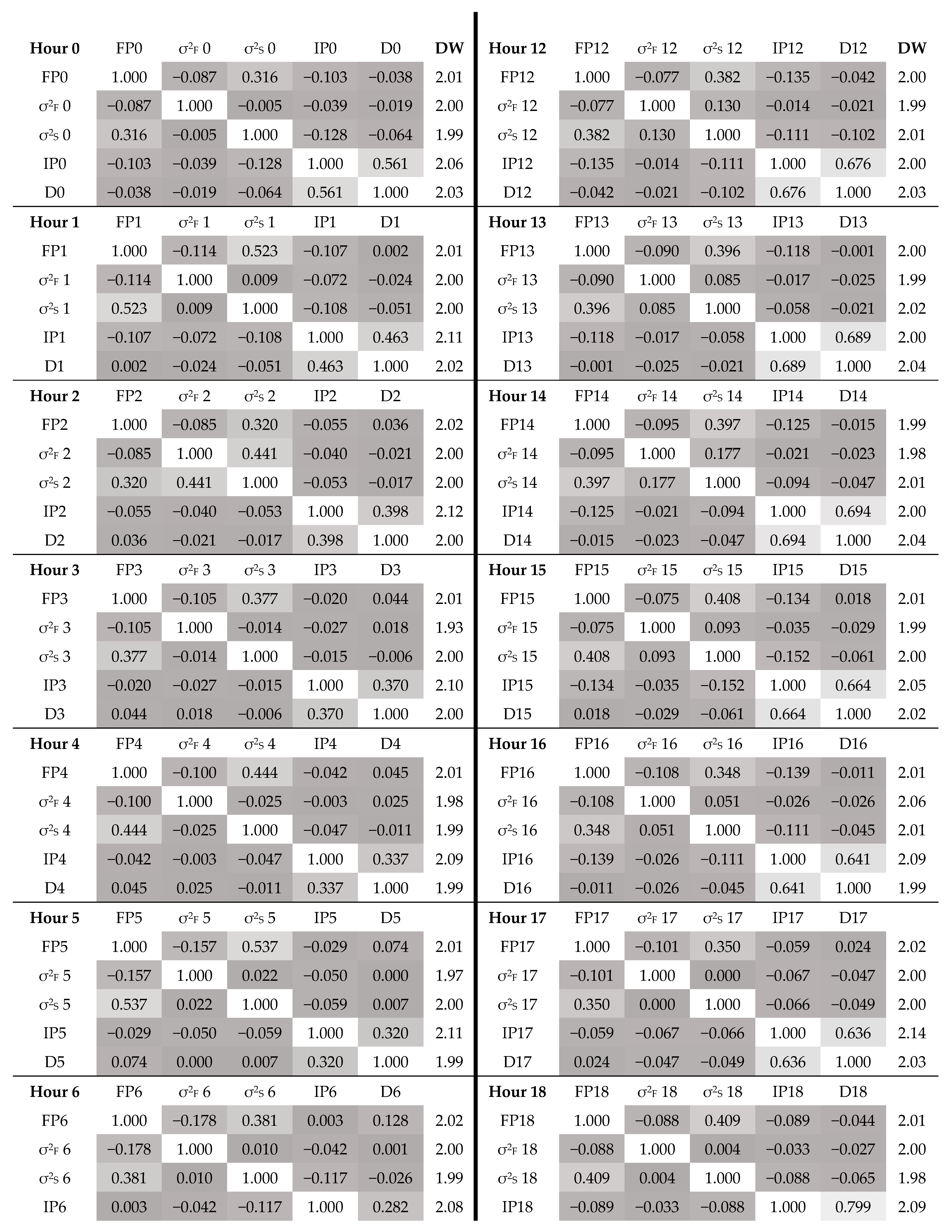
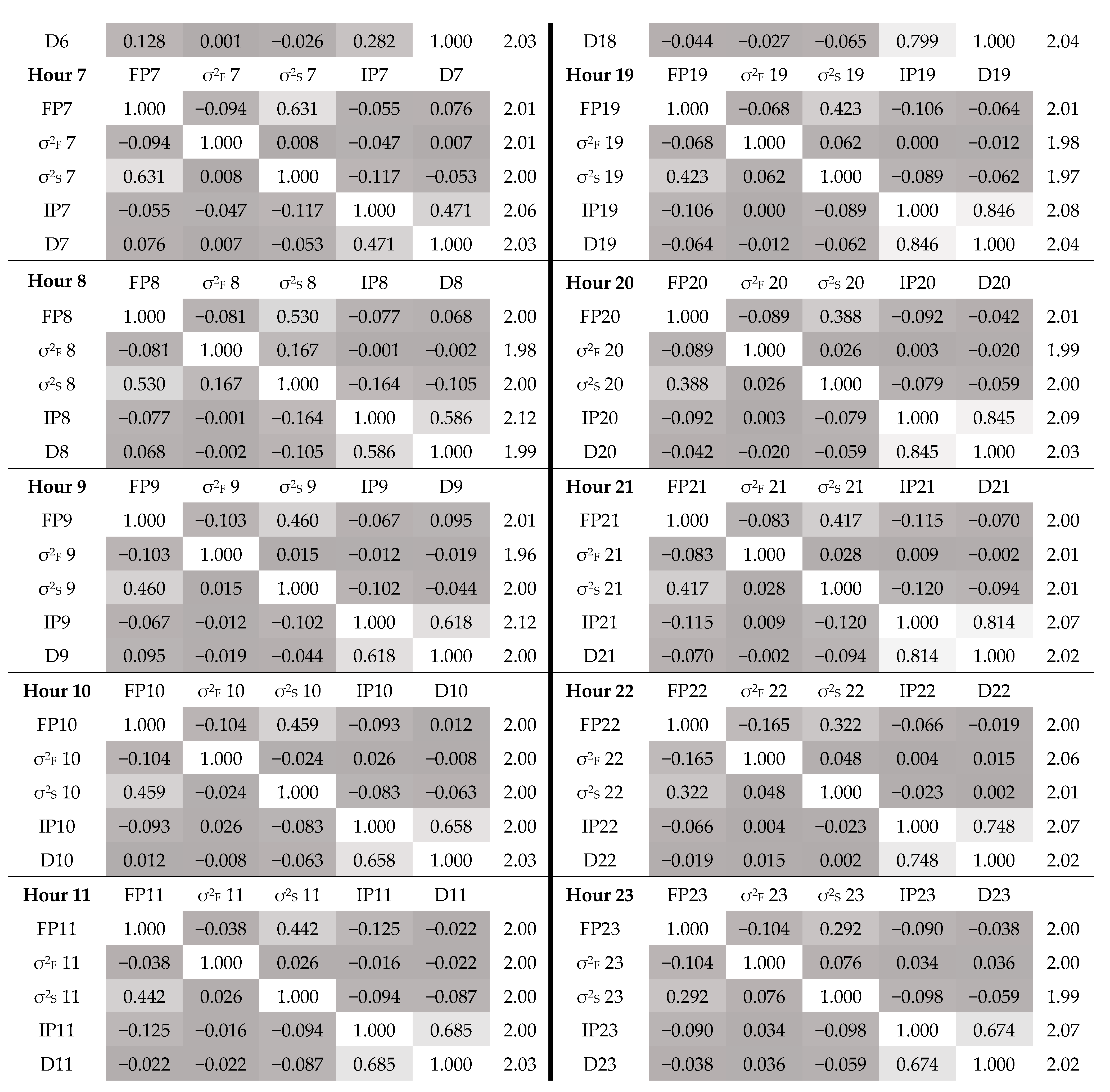
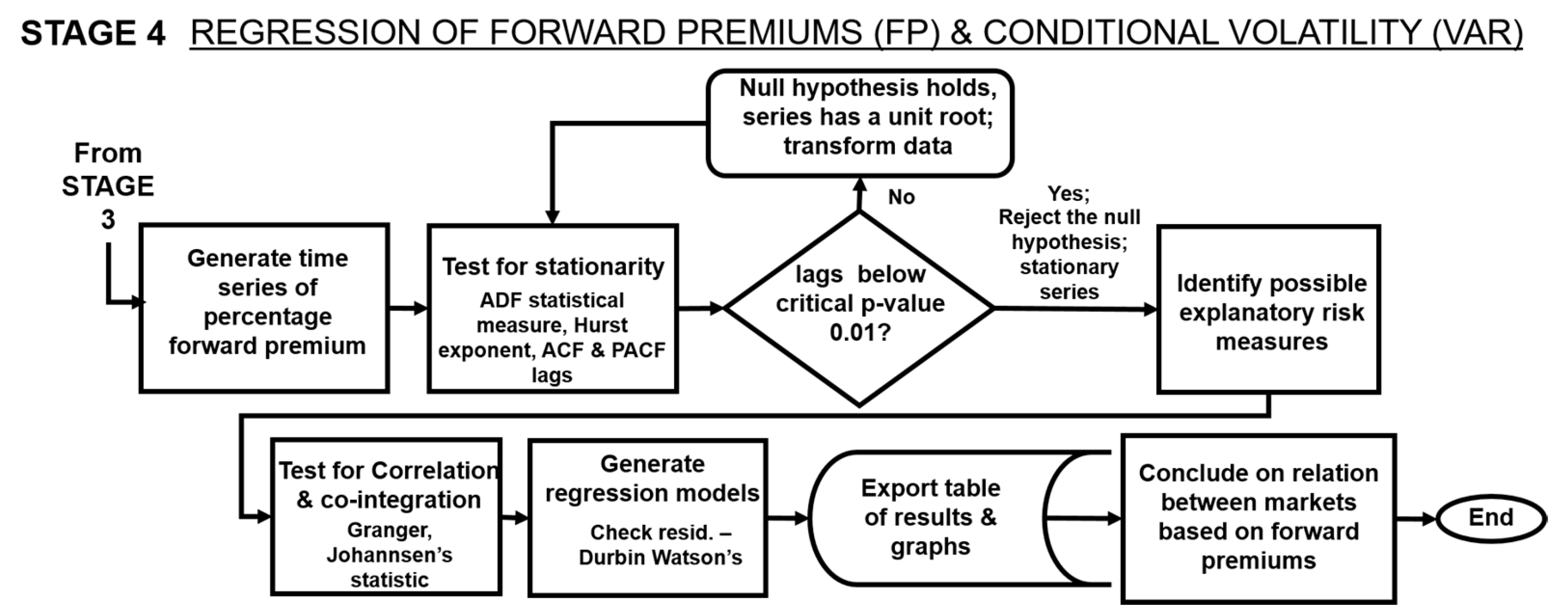
4.4. VAR Analysis for Determining the Presence of and Factors Influencing Premiums
5. Conclusions and Practical Implications
Author Contributions
Funding
Data Availability Statement
Acknowledgments
Conflicts of Interest
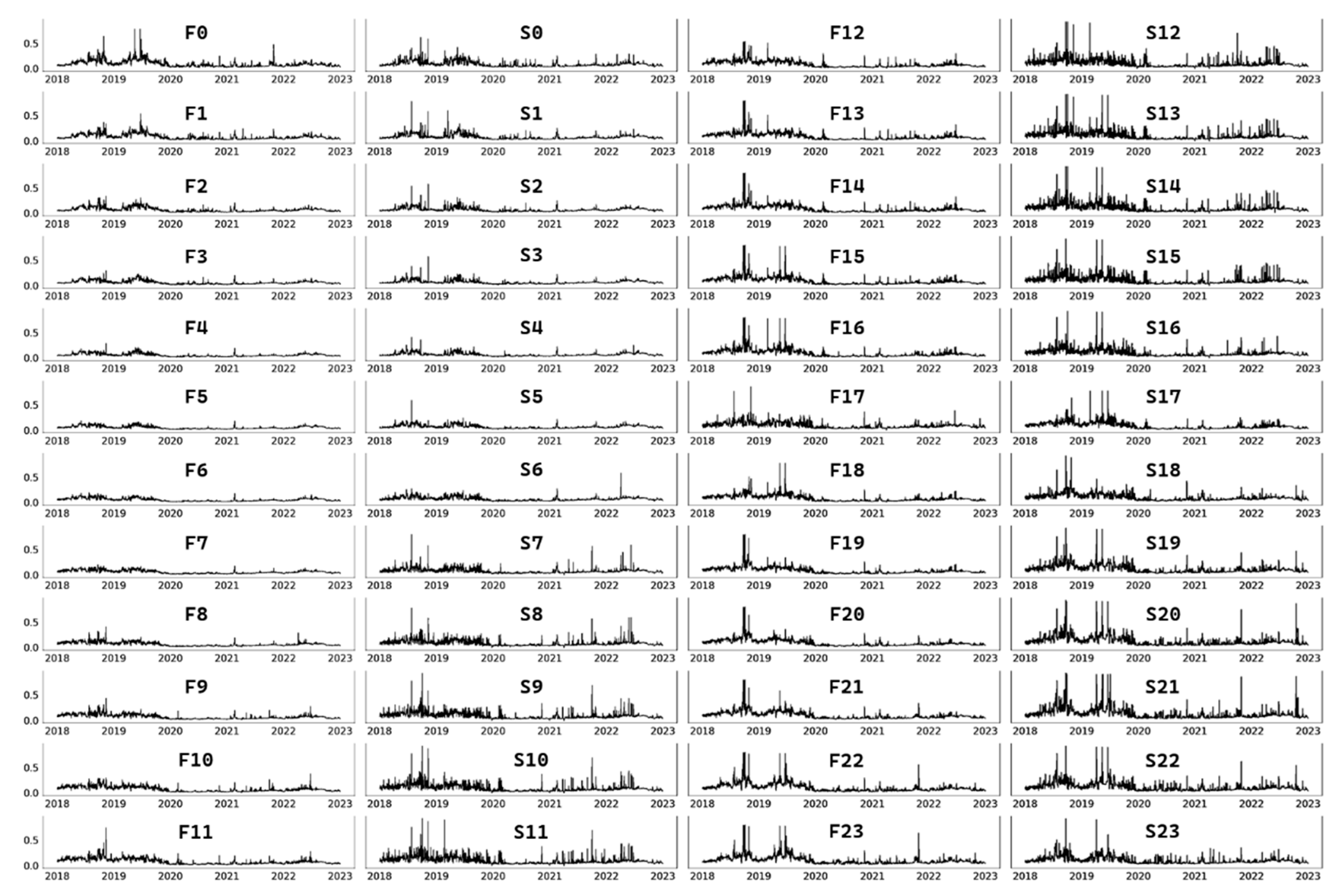
Appendix A. Forward and Spot Pricing

| Hour | Mean | Min. | Max. | Skew | Std. Deviation | |||||
|---|---|---|---|---|---|---|---|---|---|---|
| Forward | Spot | Forward | Spot | Forward | Spot | Forward | Spot | Forward | Spot | |
| 0 | 0.076 | 0.091 | 0.017 | 0.028 | 0.372 | 0.619 | 1.598 | 2.423 | 0.047 | 0.056 |
| 1 | 0.068 | 0.082 | 0.016 | 0.019 | 0.343 | 0.784 | 1.796 | 3.798 | 0.042 | 0.052 |
| 2 | 0.062 | 0.075 | 0.015 | 0.016 | 0.296 | 0.579 | 1.602 | 3.271 | 0.035 | 0.043 |
| 3 | 0.058 | 0.070 | 0.013 | 0.015 | 0.288 | 0.579 | 1.549 | 3.192 | 0.031 | 0.037 |
| 4 | 0.057 | 0.070 | 0.015 | 0.014 | 0.188 | 0.410 | 1.193 | 2.224 | 0.030 | 0.035 |
| 5 | 0.060 | 0.073 | 0.015 | 0.014 | 0.200 | 0.593 | 1.146 | 2.670 | 0.032 | 0.037 |
| 6 | 0.064 | 0.077 | 0.012 | 0.016 | 0.290 | 0.587 | 1.090 | 2.289 | 0.035 | 0.040 |
| 7 | 0.070 | 0.083 | 0.014 | 0.017 | 0.409 | 0.801 | 1.563 | 4.002 | 0.041 | 0.053 |
| 8 | 0.076 | 0.091 | 0.006 | 0.008 | 0.439 | 0.777 | 1.537 | 3.159 | 0.048 | 0.062 |
| 9 | 0.081 | 0.097 | 0.013 | 0.017 | 0.302 | 0.927 | 1.114 | 3.237 | 0.052 | 0.069 |
| 10 | 0.086 | 0.102 | 0.012 | 0.015 | 0.744 | 0.927 | 1.986 | 3.464 | 0.059 | 0.077 |
| 11 | 0.089 | 0.105 | 0.012 | 0.021 | 0.535 | 0.927 | 1.907 | 3.249 | 0.063 | 0.081 |
| 12 | 0.091 | 0.107 | 0.012 | 0.021 | 0.801 | 0.927 | 3.338 | 3.384 | 0.071 | 0.082 |
| 13 | 0.093 | 0.107 | 0.012 | 0.022 | 0.800 | 0.927 | 3.820 | 3.823 | 0.078 | 0.086 |
| 14 | 0.094 | 0.108 | 0.012 | 0.008 | 0.801 | 0.927 | 3.578 | 3.558 | 0.079 | 0.087 |
| 15 | 0.096 | 0.110 | 0.012 | 0.021 | 0.801 | 0.925 | 3.552 | 3.186 | 0.083 | 0.087 |
| 16 | 0.090 | 0.103 | 0.012 | 0.016 | 0.781 | 0.927 | 3.194 | 4.088 | 0.067 | 0.076 |
| 17 | 0.085 | 0.099 | 0.013 | 0.027 | 0.512 | 0.864 | 1.682 | 2.896 | 0.054 | 0.061 |
| 18 | 0.092 | 0.107 | 0.020 | 0.027 | 0.802 | 0.926 | 4.107 | 3.279 | 0.069 | 0.071 |
| 19 | 0.101 | 0.118 | 0.021 | 0.030 | 0.802 | 0.926 | 3.289 | 3.346 | 0.074 | 0.084 |
| 20 | 0.108 | 0.127 | 0.021 | 0.031 | 0.802 | 0.934 | 3.486 | 3.769 | 0.084 | 0.098 |
| 21 | 0.111 | 0.132 | 0.023 | 0.031 | 0.802 | 0.934 | 3.365 | 3.762 | 0.091 | 0.111 |
| 22 | 0.103 | 0.120 | 0.022 | 0.030 | 0.802 | 0.926 | 3.760 | 3.691 | 0.081 | 0.089 |
| 23 | 0.089 | 0.106 | 0.021 | 0.031 | 0.641 | 0.926 | 2.097 | 3.081 | 0.060 | 0.074 |
| (a) Forward Pricing | |||||||
|---|---|---|---|---|---|---|---|
| Hour | AR | MA | Dummy Variables | ||||
| Lag 1 | Lag 2 | Lag 3 | Lag 1 | Lag 2 | D_weekend | D_weekday | |
| 0 | 0.229 ** | −0.825 ** | −0.005 ** | 0.002 ** | |||
| 1 | 0.342 ** | −0.867 ** | −0.005 ** | 0.002 ** | |||
| 2 | 0.386 ** | −0.895 ** | |||||
| 3 | 0.372 ** | −0.869 ** | −0.003 ** | 0.001 | |||
| 4 | 0.372 ** | −0.869 ** | −0.003 ** | 0.001 | |||
| 5 | 0.287 ** | −0.829 ** | −0.004 ** | 0.002 | |||
| 6 | 0.363 ** | −0.862 ** | −0.003 ** | 0.001 | |||
| 7 | 0.405 ** | −0.895 ** | −0.002 ** | 7 × 10⁻⁴ * | |||
| 8 | 0.362 ** | −0.920 ** | |||||
| 9 | 0.586 ** | −1.171 ** | 0.216 ** | ||||
| 10 | 0.259 ** | −0.883 ** | −0.003 ** | 0.001 * | |||
| 11 | 0.348 ** | 0.099 ** | −0.937 ** | ||||
| 12 | 0.696 ** | −1.307 ** | 0.342 ** | −0.004 ** | 0.001 ** | ||
| 13 | 0.428 ** | 0.137 ** | 0.093 ** | −0.969 ** | |||
| 14 | 0.499 ** | 0.147 ** | −0.962 ** | ||||
| 15 | 0.477 ** | 0.111 ** | −0.957 ** | ||||
| 16 | 0.702 ** | −1.267 ** | 0.298 ** | ||||
| 17 | 0.230 ** | −0.892 ** | |||||
| 18 | 0.203 ** | 0.164 ** | −0.085 ** | −0.917 ** | |||
| 19 | 0.506 ** | 0.161 ** | −0.958 ** | ||||
| 20 | 0.529 ** | 0.103 ** | −0.947 ** | ||||
| 21 | 0.342 ** | −0.805 ** | |||||
| 22 | 0.205 ** | −0.756 ** | |||||
| 23 | 0.527 ** | −0.932 ** | |||||
| (b) Spot Pricing | |||||||
| Hour | AR | MA | Dummy Variables | ||||
| Lag 1 | Lag 2 | Lag 3 | Lag 1 | Lag 2 | D_weekend | D_weekday | |
| 0 | 0.345 ** | −0.931 ** | −0.010 * | 0.004 * | |||
| 1 | 0.279 ** | −0.923 ** | −0.009 * | 0.004 * | |||
| 2 | 0.302 ** | −0.910 ** | −0.009 * | 0.004 * | |||
| 3 | 0.331 ** | −0.912 ** | −0.009 * | 0.004 * | |||
| 4 | 0.436 ** | −0.913 ** | −0.007 * | 0.003 * | |||
| 5 | 0.444 ** | −0.917 ** | −0.004 * | 0.002 * | |||
| 6 | 0.378 ** | −0.923 ** | |||||
| 7 | 0.257 ** | −0.937 ** | 2 × 10⁻⁴ | −4 × 10⁻⁵ | |||
| 8 | 0.241 ** | −0.951 ** | |||||
| 9 | 0.121 ** | −0.944 ** | |||||
| 10 | 0.236 ** | −0.956 ** | |||||
| 11 | 0.148 ** | −0.951 ** | |||||
| 12 | 0.135 ** | −0.948 ** | |||||
| 13 | 0.232 ** | −0.958 ** | 0.006 * | −0.002 * | |||
| 14 | 0.257 ** | −0.952 ** | 0.009 * | −0.004 * | |||
| 15 | 0.347 ** | −0.125 ** | 0.077 ** | −0.953 ** | |||
| 16 | 0.274 ** | −0.953 ** | 0.009 ** | −0.004 ** | |||
| 17 | 0.271 ** | 0.108 ** | −0.957 ** | ||||
| 18 | 0.637 ** | −1.241 ** | 0.272 ** | ||||
| 19 | 0.460 ** | −0.950 ** | |||||
| 20 | 0.326 ** | −0.753 ** | −0.178 ** | 0.008 ** | −0.003 ** | ||
| 21 | 0.467 ** | −0.946 ** | 0.010 ** | −0.004 * | |||
| 22 | 0.278 ** | −0.729 ** | −0.207 ** | 0.008 ** | −0.003 ** | ||
| 23 | 0.607 ** | −1.212 ** | 0.249 ** | ||||
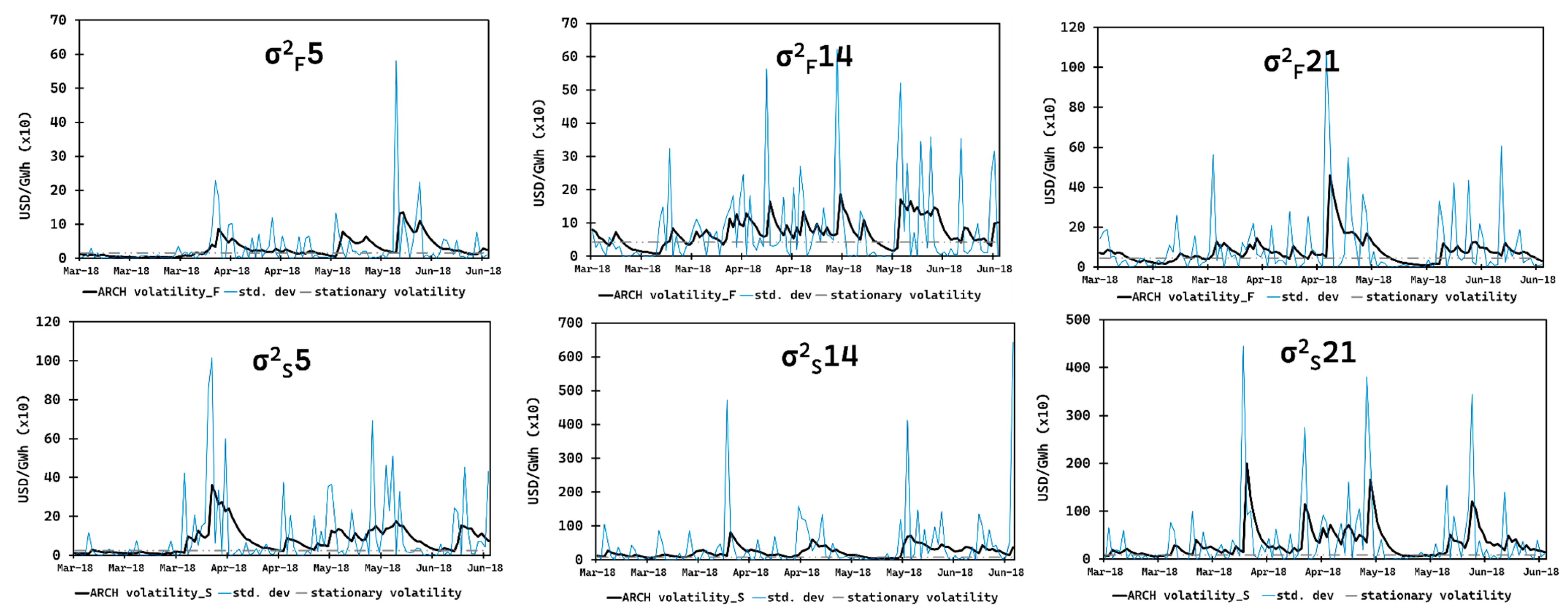
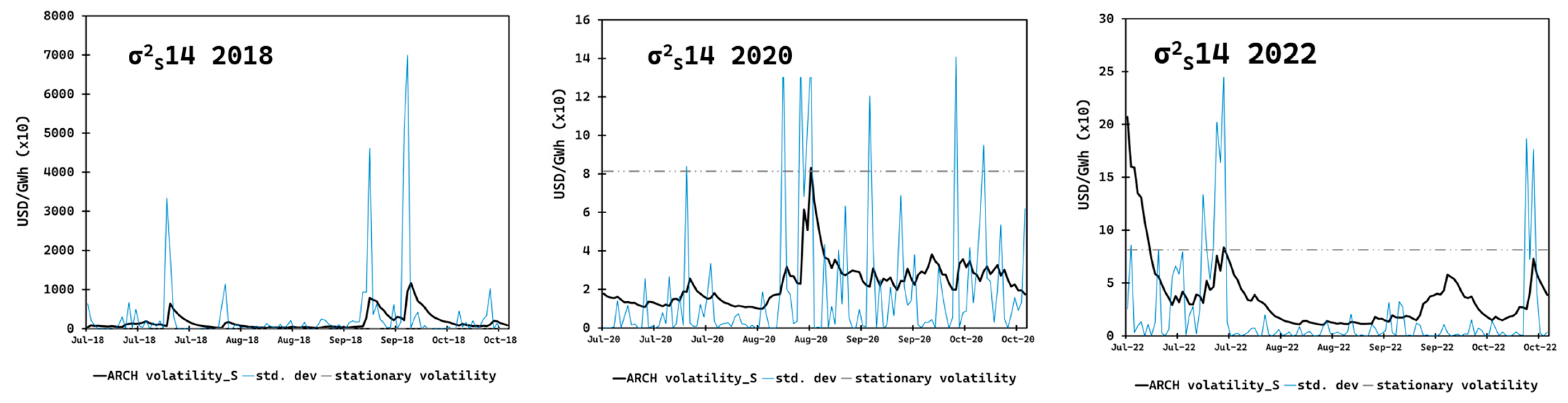
Appendix B. Volatility Modeling
| (a) Forward Pricing | |||||
|---|---|---|---|---|---|
| Hour | Model | ω | α | β | γ |
| 0 | GJR_SST | 1.9 × 10⁻¹ ** | 0.287 ** | 0.750 ** | −0.075 * |
| 1 | GJR_SST | 1.0 × 10⁻¹ ** | 0.277 ** | 0.764 ** | −0.082 ** |
| 2 | GARCH_Normal | 9.3 × 10⁻² * | 0.106 ** | 0.876 ** | |
| 3 | GARCH_SST | 2.0 × 10⁻² ** | 0.248 ** | 0.752 ** | |
| 4 | GJR_SST | 1.9 × 10⁻² ** | 0.290 ** | 0.759 ** | −0.096 ** |
| 5 | GJR_SST | 9.4 × 10⁻³ ** | 0.261 ** | 0.795 ** | −0.113 ** |
| 6 | GJR_SST | 1.0 × 10⁻² ** | 0.252 ** | 0.796 ** | −0.095 ** |
| 7 | GJR_SST | 7.7 × 10⁻³ ** | 0.229 ** | 0.816 ** | −0.090 ** |
| 8 | GARCH_SST | 1.3 × 10⁻² ** | 0.185 ** | 0.815 ** | |
| 9 | GARCH_SST | 3.6 × 10⁻² ** | 0.210 ** | 0.790 ** | |
| 10 | GARCH_SST | 4.6 × 10⁻² ** | 0.223 ** | 0.778 ** | |
| 11 | GARCH_SST | 4.0 × 10⁻² ** | 0.188 ** | 0.813 ** | |
| 12 | GARCH_SST | 1.2 × 10⁻¹ ** | 0.251 ** | 0.750 ** | |
| 13 | GJR_SST | 1.3 × 10⁻¹ ** | 0.318 ** | 0.739 ** | −0.114 ** |
| 14 | GJR_SST | 1.4 × 10⁻¹ ** | 0.338 ** | 0.730 ** | −0.136 ** |
| 15 | GJR_SST | 1.0 × 10⁻¹ ** | 0.276 ** | 0.760 ** | −0.073 ** |
| 16 | GARCH_SST | 6.0 × 10⁻² ** | 0.198 ** | 0.802 ** | |
| 17 | GARCH_SST | 4.0 × 10⁻² ** | 0.188 ** | 0.813 ** | |
| 18 | GARCH_SST | 3.3 × 10⁻² ** | 0.172 ** | 0.83 ** | |
| 19 | GJR_SST | 4.2 × 10⁻² ** | 0.267 ** | 0.787 ** | −0.108 ** |
| 20 | GJR_SST | 6.4 × 10⁻² ** | 0.315 ** | 0.755 ** | −0.140 ** |
| 21 | GJR_SST | 1.2 × 10⁻¹ ** | 0.330 ** | 0.760 ** | −0.180 ** |
| 22 | GJR_SST | 2.8 × 10⁻¹ ** | 0.351 ** | 0.734 ** | −0.169 ** |
| 23 | GJR_SST | 4.3 × 10⁻¹ ** | 0.345 ** | 0.724 ** | −0.139 ** |
| (b) Spot Pricing | |||||
| Hour | Model | ω | α | β | γ |
| 0 | GARCH_SST | 0.166 | 0.288 * | 0.712 ** | |
| 1 | GJR_SST | 0.097 * | 0.251 ** | 0.694 ** | 0.109 ** |
| 2 | GARCH_Normal | 0.065 * | 0.289 ** | 0.711 ** | |
| 3 | GARCH_SST | 0.046 ** | 0.272 ** | 0.728 ** | |
| 4 | GARCH_SST | 0.040 ** | 0.225 ** | 0.775 ** | |
| 5 | GJR_SST | 0.030 ** | 0.231 ** | 0.799 ** | −0.060 ** |
| 6 | GARCH_SST | 0.029 ** | 0.188 ** | 0.812 ** | |
| 7 | GJR_SST | 0.131 * | 0.170 ** | 0.767 ** | 0.126 ** |
| 8 | GJR_SST | 0.166 ** | 0.152 ** | 0.791 ** | 0.113 ** |
| 9 | GARCH_SST | 0.220 ** | 0.178 ** | 0.822 ** | |
| 10 | GJR_SST | 0.329 ** | 0.156 ** | 0.777 ** | 0.134 ** |
| 11 | GJR_SST | 0.309 ** | 0.101 ** | 0.807 ** | 0.185 ** |
| 12 | GJR_SST | 0.260 ** | 0.010 ** | 0.814 ** | 0.174 ** |
| 13 | GJR_SST | 0.268 ** | 0.148 ** | 0.772 ** | 0.159 ** |
| 14 | GJR_SST | 0.207 * | 0.175 ** | 0.762 ** | 0.127 ** |
| 15 | GJR_SST | 0.167 ** | 0.187 ** | 0.778 ** | 0.070 ** |
| 16 | GJR_SST | 0.115 ** | 0.156 ** | 0.791 ** | 0.105 ** |
| 17 | GJR_SST | 0.063 * | 0.155 ** | 0.823 ** | 0.045 * |
| 18 | GARCH_SST | 0.116 * | 0.234 ** | 0.766 ** | |
| 19 | GARCH_SST | 0.498 ** | 0.318 ** | 0.682 ** | |
| 20 | GJR_SST | 1.510 ** | 0.442 ** | 0.621 ** | −0.126 ** |
| 21 | GJR_SST | 1.450 ** | 0.453 ** | 0.627 ** | −0.159 ** |
| 22 | GJR_SST | 1.930 ** | 0.561 ** | 0.525 ** | −0.172 ** |
| 23 | GJR_SST | 1.040 ** | 0.509 ** | 0.557 ** | −0.131 ** |
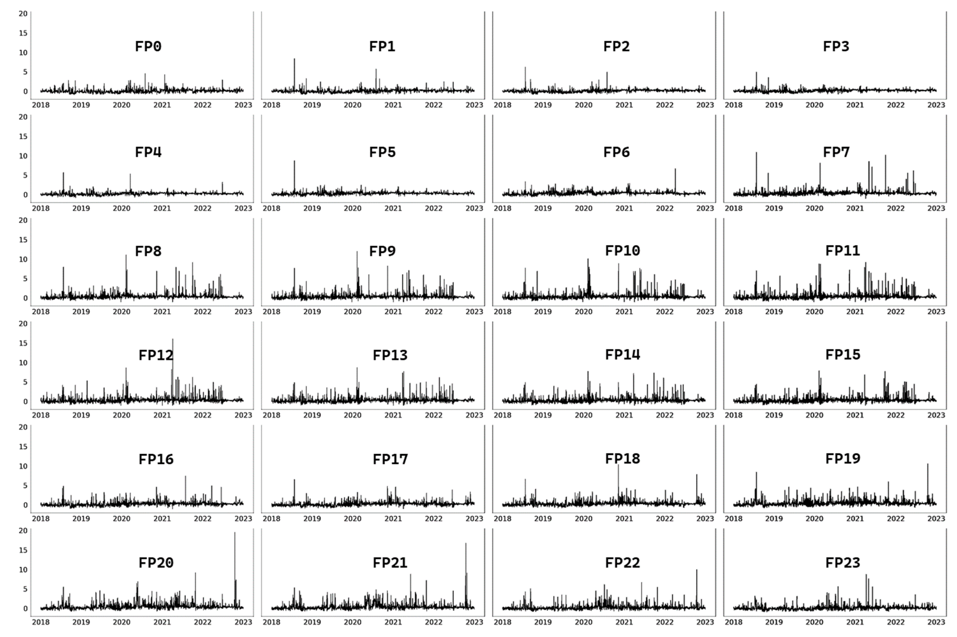
Appendix C. Vector Autoregression Modeling
| Hour | Average | Skew | Std. Deviation |
|---|---|---|---|
| 0 | 0.07 | 2.17 | 0.47 |
| 1 | 0.10 | 4.80 | 0.47 |
| 2 | 0.14 | 3.46 | 0.41 |
| 3 | 0.18 | 2.04 | 0.37 |
| 4 | 0.25 | 3.59 | 0.38 |
| 5 | 0.34 | 5.52 | 0.41 |
| 6 | 0.39 | 2.68 | 0.46 |
| 7 | 0.42 | 6.86 | 0.71 |
| 8 | 0.44 | 5.85 | 0.79 |
| 9 | 0.43 | 5.13 | 0.82 |
| 10 | 0.41 | 5.01 | 0.87 |
| 11 | 0.40 | 4.66 | 0.88 |
| 12 | 0.37 | 6.37 | 0.85 |
| 13 | 0.34 | 4.07 | 0.74 |
| 14 | 0.32 | 3.88 | 0.73 |
| 15 | 0.34 | 3.89 | 0.73 |
| 16 | 0.28 | 3.12 | 0.61 |
| 17 | 0.27 | 2.71 | 0.57 |
| 18 | 0.38 | 4.45 | 0.67 |
| 19 | 0.48 | 3.76 | 0.75 |
| 20 | 0.51 | 6.85 | 0.93 |
| 21 | 0.45 | 5.52 | 0.92 |
| 22 | 0.28 | 3.86 | 0.73 |
| 23 | 0.15 | 4.40 | 0.63 |


References
- De Rosa, M.; Gainsford, K.; Pallonetto, F.; Finn, D.P. Diversification, concentration and renewability of the energy supply in the European Union. Energy 2022, 253, 124097. [Google Scholar] [CrossRef]
- Burke, P.J. Income, resources, and electricity mix. Energy Econ. 2010, 32, 616–626. [Google Scholar] [CrossRef]
- Do, T.N.; Burke, P.J. Is ASEAN ready to move to multilateral cross-border electricity trade? Asia Pac. Viewp. 2023, 64, 110–125. [Google Scholar] [CrossRef]
- Chen, F.; Huang, K.; Hou, Y.; Ding, T. Long-term cross-border electricity trading model under the background of Global Energy Interconnection. Glob. Energy Interconnect. 2019, 2, 122–129. [Google Scholar] [CrossRef]
- Oseni, M.O.; Pollitt, M.G. The promotion of regional integration of electricity markets: Lessons for developing countries. Energy Policy 2016, 88, 628–638. [Google Scholar] [CrossRef]
- Haque, H.M.E.; Dhakal, S.; Mostafa, S.M.G. An assessment of opportunities and challenges for cross-border electricity trade for Bangladesh using SWOT-AHP approach. Energy Policy 2020, 137, 111118. [Google Scholar] [CrossRef]
- Dhakal, S.; Karki, P.; Shrestha, S. Cross-border electricity trade for Nepal: A SWOT-AHP analysis of barriers and opportunities based on stakeholders’ perception. Int. J. Water Resour. Dev. 2021, 37, 559–580. [Google Scholar] [CrossRef]
- Thaler, P.; Hofmann, B. The impossible energy trinity: Energy security, sustainability, and sovereignty in cross-border electricity systems. Polit. Geogr. 2022, 94, 102579. [Google Scholar] [CrossRef]
- Yuan, M.; Tapia-Ahumada, K.; Reilly, J. The role of cross-border electricity trade in transition to a low-carbon economy in the Northeastern U.S. Energy Policy 2021, 154, 112261. [Google Scholar] [CrossRef]
- IEA. Mexico—Countries & Regions—IEA. 2024. Available online: https://www.iea.org/countries/mexico/electricity (accessed on 20 February 2024).
- Office of the United States Trade Representative. The United States of America, the United Mexican States, and Canada Trade Agreement 7/1/20 Text|United States Trade Representative. 2023. Available online: https://ustr.gov/trade-agreements/free-trade-agreements/united-states-mexico-canada-agreement/agreement-between (accessed on 20 February 2024).
- Sarmiento, L.; Molar-Cruz, A.; Avraam, C.; Brown, M.; Rosellón, J.; Siddiqui, S.; Rodríguez, B.S. Mexico and U.S. power systems under variations in natural gas prices. Energy Policy 2021, 156, 112378. [Google Scholar] [CrossRef]
- Belize Electricity Limited. Belize Electricity Limited Annual Report 2022. Belize, 2022. Available online: https://indd.adobe.com/view/8fd0b2f4-532b-4a25-b5e8-478794c11a0b (accessed on 26 September 2023).
- Guderjan, T.; Beach, T.; Luzzadder-Beach, S.; Bozarth, S. Understanding the Causes of Abandonment in the Maya Lowlands. Archaeol. Rev. Camb. 2009, 24, 99–121. Available online: https://www.researchgate.net/publication/281572917_Understanding_the_causes_of_abandonment_in_the_Maya_Lowlands (accessed on 6 September 2023).
- IEA. Electricity—Energy System—IEA. 2023. Available online: https://www.iea.org/energy-system/electricity (accessed on 6 September 2023).
- Tillett, A.; Locke, J.; Mencias, J. Belize National Energy Policy Framework. Natl. Energy Policy 2011. Available online: https://www.publicservice.gov.bz/index.php/medias/news-and-events/download/11/56/15 (accessed on 6 September 2023).
- Percino-Picazo, J.C.; Llamas-Terres, A.R.; Viramontes-Brown, F.A. Analysis of Restructuring the Mexican Electricity Sector to Operate in a Wholesale Energy Market. Energies 2021, 14, 3331. [Google Scholar] [CrossRef]
- De la Torre, J.; Rodriguez, L.R.; Monteagudo, F.E.L.; Arredondo, L.R.; Enriquez, J.B. Electricity price forecast in wholesale markets using conformal prediction: Case study in Mexico. Energy Sci. Eng. 2024, 12, 524–540. [Google Scholar] [CrossRef]
- Algieri, B.; Leccadito, A.; Tunaru, D. Risk premia in electricity derivatives markets. Energy Econ. 2021, 100, 105300. [Google Scholar] [CrossRef]
- Wei, W.; Lunde, A. Identifying Risk Factors and Their Premia: A Study on Electricity Prices. J. Financ. Econom. 2022, 21, 1647–1679. [Google Scholar] [CrossRef]
- Fama, E.F. Efficient Capital Markets: A Review of Theory and Empirical Work. J. Financ. 1970, 25, 383. [Google Scholar] [CrossRef]
- Longstaff, F.A.; Wang, A.W. Electricity Forward Prices: A High-Frequency Empirical Analysis. J. Financ. 2004, 59, 1877–1900. [Google Scholar] [CrossRef]
- Koten, S. Van Forward premia in electricity markets: A replication study. Energy Econ. 2020, 89, 104812. [Google Scholar] [CrossRef]
- Ramírez-García, A.; Saucedo, E.; Ramírez-García, A.; Saucedo, E. Hedging Electricity Price Volatility Applying Seasonal and Trend Decomposition. Análisis Económico 2022, 37, 143–166. [Google Scholar] [CrossRef]
- Cruz May, E.; Bassam, A.; Ricalde, L.J.; Escalante Soberanis, M.A.; Oubram, O.; May Tzuc, O.; Alanis, A.Y.; Livas-García, A. Global sensitivity analysis for a real-time electricity market forecast by a machine learning approach: A case study of Mexico. Int. J. Electr. Power Energy Syst. 2022, 135, 107505. [Google Scholar] [CrossRef]
- Rodriguez-Aguilar, R.; Marmolejo-Saucedo, J.A.; Retana-Blanco, B. Prices of Mexican Wholesale Electricity Market: An Application of Alpha-Stable Regression. Sustainability 2019, 11, 3185. [Google Scholar] [CrossRef]
- Livas-García, A.; May Tzuc, O.; Cruz May, E.; Tariq, R.; Jimenez Torres, M.; Bassam, A. Forecasting of locational marginal price components with artificial intelligence and sensitivity analysis: A study under tropical weather and renewable power for the Mexican Southeast. Electr. Power Syst. Res. 2022, 206, 107793. [Google Scholar] [CrossRef]
- Box, G.E.; Jenkins, G.M.; Reinsel, G.C.; Ljung, G.M. Time Series Analysis: Forecasting and Control; John Wiley & Sons: Hoboken, NJ, USA, 2015. [Google Scholar]
- Bollerslev, T. Generalized autoregressive conditional heteroskedasticity. J. Econom. 1986, 31, 307–327. [Google Scholar] [CrossRef]
- Wang, D.; Gryshova, I.; Kyzym, M.; Salashenko, T.; Khaustova, V.; Shcherbata, M. Electricity Price Instability over Time: Time Series Analysis and Forecasting. Sustainability 2022, 14, 9081. [Google Scholar] [CrossRef]
- Ioannidis, F.; Kosmidou, K.; Savva, C.; Theodossiou, P. Electricity pricing using a periodic GARCH model with conditional skewness and kurtosis components. Energy Econ. 2021, 95, 105110. [Google Scholar] [CrossRef]
- Janczura, J.; Puć, A. ARX-GARCH Probabilistic Price Forecasts for Diversification of Trade in Electricity Markets—Variance Stabilizing Transformation and Financial Risk-Minimizing Portfolio Allocation. Energies 2023, 16, 807. [Google Scholar] [CrossRef]
- Ahmad, T.I.; Kiran, K.; Alamgir, A. Households’ Clean Cooking Fuel Poverty: Testing the Energy-Ladder Hypothesis in the Case of Bangladesh. iRASD J. Energy Environ. 2023, 4, 42–55. [Google Scholar] [CrossRef]
- Viehmann, J. Risk premiums in the German day-ahead Electricity Market. Energy Policy 2011, 39, 386–394. [Google Scholar] [CrossRef]
- National Centers for Environmental Information. Past Weather | National Centers for Environmental Information (NCEI). 2024. Available online: https://www.ncei.noaa.gov/access/past-weather/22.16799201091221,-94.84984515217047,16.93260562480587,-84.65998763121615 (accessed on 5 January 2024).
- EIA. Henry Hub Natural Gas Spot Price (Dollars per Million Btu). 2024. Available online: https://www.eia.gov/dnav/ng/hist/rngwhhdD.htm (accessed on 10 January 2024).
- CENACE. Estimation of Actual Demand—Wholesale Electricity Market (MEM). 2024. Available online: https://www.cenace.gob.mx/Paginas/SIM/Reportes/EstimacionDemandaReal.aspx (accessed on 23 February 2024).
- Perktold, J.; Skipper, S.; Taylor, J. Augmented Dickey-Fuller Unit Root-Test, statsmodels.tsa.stattools.adfuller—statsmodels 0.15.0 (+213); 2024. Available online: https://www.statsmodels.org/dev/generated/statsmodels.tsa.stattools.adfuller.html (accessed on 28 February 2024).
- Dickey, D.A.; Fuller, W.A. Likelihood Ratio Statistics for Autoregressive Time Series with a Unit Root. Econometrica 1981, 49, 1057. [Google Scholar] [CrossRef]
- Smith, T.G. pmdarima 2.0.4 API Reference, pmdarima.arima.auto_arima—pmdarima 2.0.4 documentation; 2023. Available online: https://alkaline-ml.com/pmdarima/modules/generated/pmdarima.arima.auto_arima.html (accessed on 28 February 2024).
- Breusch, T.S.; Pagan, A.R. The Lagrange Multiplier Test and its Applications to Model Specification in Econometrics. Rev. Econ. Stud. 1980, 47, 239. [Google Scholar] [CrossRef]
- Nugroho, D.B.; Priyono, A.; Susanto, B. Skew normal and skew student-t distributions on GARCH(1,1) model. Media Stat. 2021, 14, 21–32. [Google Scholar] [CrossRef]
- Hacker, R.S.; Hatemi-J, A. Optimal lag-length choice in stable and unstable VAR models under situations of homoscedasticity and ARCH. J. Appl. Stat. 2008, 35, 601–615. [Google Scholar] [CrossRef]
- statsmodels 0.14.1. Time Series Analysis Tsa—statsmodels 0.14.1. 2024. Available online: https://www.statsmodels.org/stable/tsa.html (accessed on 19 April 2024).
- Durbin, J.; Watson, G.S. Testing for serial correlation in least squares regression. I. Biometrika 1950, 37, 409–428. [Google Scholar] [CrossRef] [PubMed]
- Granger, C.W.J. Investigating Causal Relations by Econometric Models and Cross-spectral Methods. Econometrica 1969, 37, 424. [Google Scholar] [CrossRef]
- Johansen, S. Estimation and Hypothesis Testing of Cointegration Vectors in Gaussian Vector Autoregressive Models. Econometrica 1991, 59, 1551. [Google Scholar] [CrossRef]
- Valitov, N. Risk premia in the German day-ahead electricity market revisited: The impact of negative prices. Energy Econ. 2019, 82, 70–77. [Google Scholar] [CrossRef]
- Bessembinder, H.; Lemmon, M.L. Equilibrium Pricing and Optimal Hedging in Electricity Forward Markets. J. Finance 2002, 57, 1347–1382. [Google Scholar] [CrossRef]

| Hour | ∅1 | ∅2 | ∅3 | ∅4 |
|---|---|---|---|---|
| 0 | −9%∆ * | 32%∆ * | −10% * | −4% |
| 1 | −11%∆ * | 52%∆ * | −11%∆ * | 0% |
| 2 | −8%∆ * | 32%∆ * | −5% * | 4% |
| 3 | −10%∆ * | 38%∆ * | −2% * | 4% |
| 4 | −10%∆ * | 44%∆ * | −4% * | 4% |
| 5 | −16%∆ * | 54%∆ * | −3% * | 7% |
| 6 | −18%∆ * | 38%∆ * | 0%∆ * | 13%∆ |
| 7 | −9%∆ * | 63%∆ * | −6%∆ * | 8%∆ |
| 8 | −8%∆ * | 53%∆ * | −8%∆ * | 7%∆ * |
| 9 | −10%* | 46%∆ * | −7%∆ * | 10%∆ * |
| 10 | −10%∆ * | 46%∆ * | −9%∆ * | 1%∆ * |
| 11 | −4%∆ * | 44%∆ * | −13%∆ * | −2%∆ * |
| 12 | −8%∆ * | 38%∆ * | −14%∆ * | −4%∆ * |
| 13 | −9%∆ * | 40%∆ * | −12%∆ * | 0% * |
| 14 | −9%∆ * | 40%∆ * | −13%∆ * | −2%∆ * |
| 15 | −7%∆ * | 41%∆ * | −13%∆ * | 2%∆ * |
| 16 | −11%∆ * | 35%∆ * | −14%∆ * | −1% * |
| 17 | −10%∆ * | 35%∆ * | −6% * | 2%* |
| 18 | −9%∆ * | 41%∆ * | −9% * | −4% |
| 19 | −7%∆ * | 42%∆ * | −11%∆ * | −6% |
| 20 | −9%∆ * | 39%∆ * | −9%∆ * | −4%∆ |
| 21 | −8%∆ * | 42%∆ * | −11% * | −7%∆ * |
| 22 | −16%∆ * | 32%∆ * | −7% * | −2% * |
| 23 | −10%∆ * | 29%∆ * | −9% * | −4% * |
Disclaimer/Publisher’s Note: The statements, opinions and data contained in all publications are solely those of the individual author(s) and contributor(s) and not of MDPI and/or the editor(s). MDPI and/or the editor(s) disclaim responsibility for any injury to people or property resulting from any ideas, methods, instructions or products referred to in the content. |
© 2024 by the authors. Licensee MDPI, Basel, Switzerland. This article is an open access article distributed under the terms and conditions of the Creative Commons Attribution (CC BY) license (https://creativecommons.org/licenses/by/4.0/).
Share and Cite
Usher, K.S.; McLellan, B.C. Price Risk Exposure of Small Participants in Liberalized Multi-National Power Markets: A Case Study on the Belize–Mexico Interconnection. Energies 2024, 17, 3464. https://doi.org/10.3390/en17143464
Usher KS, McLellan BC. Price Risk Exposure of Small Participants in Liberalized Multi-National Power Markets: A Case Study on the Belize–Mexico Interconnection. Energies. 2024; 17(14):3464. https://doi.org/10.3390/en17143464
Chicago/Turabian StyleUsher, Khadija Sherece, and Benjamin Craig McLellan. 2024. "Price Risk Exposure of Small Participants in Liberalized Multi-National Power Markets: A Case Study on the Belize–Mexico Interconnection" Energies 17, no. 14: 3464. https://doi.org/10.3390/en17143464