Transformation towards a Low-Emission and Energy-Efficient Economy Realized in Agriculture through the Increase in Controllability of the Movement of Units Mowing Crops While Simultaneously Discing Their Stubble

Abstract

When harvesting cereals and fodder grasses, a two-phase method is often used. This process is carried out using trailed and suspended collecting units. The former are asymmetrical and often pose problems regarding the stability of their movement in the horizontal plane. In practice, suspended harvesting units with a front-mounted header are becoming more and more widely used. The disadvantage of their use is that the soil is exposed after passing through the space between the swaths of the mown crop. This is followed by an intense loss of moisture. In order to eliminate this shortcoming, a collecting unit was proposed, consisting of a tractor with a front attachment and a disc harrow mounted at the rear. An appropriate mathematical model was developed to justify the scheme and parameters of such a unit. In this case, this model is used to assess the controllability of the movement of the dynamic system under the influence of control action in the form of the angular rotation of the tractor’s steered wheels. As a result of mathematical modelling, it was found that satisfactory controllability of the movement of the harvesting units can be ensured by acting on the tractor’s driven wheels with a frequency of 0–1 s⁻¹ and a working speed of close to 3 m·s⁻¹. In this case, it is desirable to set the deflection resistance coefficient of the rear tyres of the tractor (and therefore, the air pressure in them) to a smaller value, and that of the front tyres to a larger value. This helps both to improve the movement controllability of the harvesting unit and to reduce its energy consumption by an average of 6.75%. The emissivity of selected harmful chemicals and particulates emitted by the harvesting unit, depending on the fuel burned, was also examined. The way in which the use of the harvesting unit affects the reduction of emissions of harmful compounds into the atmosphere was also revealed.

1. Introduction

The Earth’s limited natural resources, climate change, and the issue of providing food for an increasing human population with limited access to water and arable land are the main challenges faced by modern agriculture [1,2,3]. For many years, the concept of sustainable agriculture has appeared in the nomenclature. This term refers to all measures that reduce the environmental impact of agriculture, which are intended to enable a more efficient and environmentally friendly use of resources, such as soil, land, water, agricultural machinery, plant protection products, seeds, fertilisers, or energy, while maintaining the profitability of agricultural production and its social acceptance [4,5].

Sustainable agriculture is a trade-off that offers to reduce the negative impact on the environment and the climate while sustaining an adequate production scale and maintaining the financial stability of the farms. The sustainable farm management model does not guarantee an increase in profits here and now, but allows for the economic stability of agricultural activity over a longer period of time. This is extremely important in terms of the model’s resilience to all crises affecting both local and global economies. The implementation of the concept of sustainable agricultural production requires a number of organisational and technological adaptations, specifically the basic elements of technology, such as fertility, fertilisers, and plant protection [6,7].

Climate change brings increasingly unpredictable and extreme weather, and farmers find it difficult to adapt to these new climatic conditions [8,9]. An increasing number of European legislators claim that the development of genetically modified supercrops may be a way to ensure food security. The research aims to modify such crops to require less water, fewer pesticides and fertilizers, and to be more resilient to climate change [10,11]. The EU has some of the strictest regulations in the world for the approval of GM crops, and the development of GMOs (genetically modified organisms) remains a contentious issue among both governments and citizens [12,13].

The primary objective of every producer in the traditional (classical) management system was to maximise profit, while sometimes ignoring the principles of good agricultural practice, which is the basis of sustainable agriculture [14,15]. The current knowledge and skills make it possible to achieve these goals by applying integrated agricultural production technologies in accordance with the principles of sustainable agriculture [16,17].

The growing demand for high-quality plant products and changing customer requirements motivate farms to change, specialize, and increasingly use modern solutions and equipment. Thanks to these innovations, the harvest is much more abundant, and the work is less tiring and more effective [18]. The elements of agrotechnics in regards to plough technology, such as tillage, fertilization, and care, are both energy- and time-consuming [19]. For many years, in the scientific community and among farmers, there has been a debate over whether classic plough or no-till cultivation, or perhaps even direct sowing, is better. It is impossible to unequivocally determine which cultivation technology is better. Any method is good and effective if it delivers the intended results and savings. Therefore, in modern agriculture, new technologies, machinery, GSP satellite navigation, modern plant protection products, and fertilisers are introduced, which reduce costs. The choice of an arable farming system depends on the size of the farm, the physicochemical and biological properties of the soil, the landscape, the climate, the crop, and of course, the approach of the farmer and the degree to which he wants to use modern technologies [20].

Of all the known methods of harvesting crops, two are currently used most often: single-phase and two-phase harvesting. Studies show that there are both advantages and disadvantages to harvesting rapeseed [21] and other crops [22]. In this regard, the prevailing climatic conditions determine the methods of choice in a particular geographical area.

The two-phase method of harvesting is widely used when mowing cereal crops, forage grasses, and rapeseed. For this process, trailed and mounted harvesting units are used. The former consists of a tractor with a trailed header asymmetrically placed on the right [23,24,25]. One of the significant problems with using such units is their reduced stability of movement in the horizontal plane [26]. Studies have shown [27] that this fact has a corresponding effect on the quality of the harvesting process.

Mounted units are equipped with front headers, which are joined to a self-propelled power device (combine, tractor), both symmetrically and asymmetrically. In a symmetrical harvesting unit [28,29,30,31], the crop swath is located between the wheels of the left and right sides of the self-propelled vehicle.

When a cut crop swath forms to the left or right of a front-mounted header, the latter is usually attached to the self-propelled vehicle asymmetrically [22,32,33]. However, its transverse displacement usually does not cause problems with the stability of the harvesting unit’s horizontal movement. After the latter’s passage, the stubble of the harvested crop remains. To avoid moisture loss and achieve weed control, most often, after 2–3 days, the stubble is crushed by disc cultivators (harrows) during the subsequent tillage to a depth of 5–7 cm.

Crushing the harvested crop stubble is not carried out using the no-till technology. Moreover, in its inter-rows, there is a non-grain portion of the crop. As a result, this contributes to increased soil moisture infiltration and other positive effects [34]. In some cases, the stubble remains intact throughout the winter, contributing to the effective retention of snow in the fields [35].

Nevertheless, it should be noted that under arid soil and climatic conditions, a delay in chopping the stubble of a harvested crop, even of only 2–3 days, can lead to significant losses of soil moisture. At the same time, according to field studies, the timely implementation of this technological operation makes it possible to ensure moisture conservation in the soil within 2–6 mm [36]. Moreover, its subsequent accumulation increases significantly when the stubble is crushed simultaneously with its mowing.

Soil moisture can be defined in many ways. The International Hydrological Dictionary describes it as water contained in the aeration zone above the groundwater table, together with water vapor present in the soil pores [37,38].

Soil water resources are a major topic of research interest. All processes that take place in the soil are strongly linked to its moisture, and therefore, the measurement of water content in the soil is one of the most important problems in agrotechnology and issues related to the formation of optimal conditions for the growth and development of plants [39,40].

The changing hydrological situation of the world and the ongoing work on the assessment of soil water resources have led to rapid progress in the development of measurement methods. Starting with the traditional thermogravimetric method, commonly called “drying”, the development of measurement methods has led to more advanced techniques, which include: TDR (time domain reflectometry), FDR (frequency domain reflectometry), as well as capacitance, neutron, or electrometric (resistance) measurement. The choice of a suitable method for monitoring soil moisture is determined primarily by features such as high measurement accuracy, the possibility of continuous measurements in many places simultaneously, non-destructive characteristics, and a relatively low cost of measuring equipment. Methods based on electrostatic conductivity phenomena are becoming increasingly popular for field measurements [41].

The physical state of the soil depends on natural and anthropogenic factors that contribute to changing the state of soil density. Soil penetration resistance is a valuable indicator of soil mechanical resistance during plant root growth. Soil penetration resistance largely depends on the method of cultivation. Penetration resistance also depends, to a significant extent, on soil moisture; therefore, in order to assess the impact of different cultivation methods on soil mechanical resistance, it is necessary to determine the relationship between moisture and soil penetration resistance, taking into account the agrotechnical practices used and the cultivation methods shaping the structure and state of soil compaction [42].

There are known attempts to implement this technological technique as unit in a combined harvester and a trailed cultivator [43]. But the latter’s presence significantly complicates the reverse movement of such a harvesting unit when manoeuvring on the headland. Moreover, the motion dynamics of such a dynamic system have not been studied, which is why neither its diagram nor its design parameters are substantiated.

It should be noted that unsatisfactory unit controllability is clearly associated with increased fuel consumption. The related increased energy consumption requires the identification of ways to reduce it. However, practically no studies reflect the influence of the units’ movement controllability (including that required during harvesting) on fuel consumption (and, therefore, energy).

Our experience tells us that the front harvester and rear tillage machine must be mounted. At the same time, if the first machine (header) should possess only a fixed device, then the second apparatus (harrow, cultivator) can include both a fixed and an articulated joint in a horizontal plane with a self-propelled vehicle. The latter can be equipped with both front- and rear-steered wheels. However, an appropriate mathematical formula is needed to theoretically study such a unit’s movement dynamics. Since it is currently missing, the aim of this article is: (i) to design a mathematical model of the combined harvesting unit’s horizontal movement; (ii) to assess the unit movement controllability, based on a self-propelled vehicle with a front-mounted header and a soil-cultivating machine mounted at the rear; (iii) to assess the influence of the harvesting unit’s movement controllability on its energy consumption.

2. Theoretical Premises

In practice, two diagrams of a harvesting unit are possible: a straight-path tractor, and a front header with a rear-mounted disc harrow. According to the first of these diagrams, the tractor (following the example of a combine) has rear-steered wheels. Technically, this is achieved by setting it to reverse. According to the second diagram, the tractor moves in a straight line with front-steered wheels (Figure 1). In both diagrams of the harvesting unit, the disc harrow is mounted with the possibility of its independent rotation in the horizontal plane relative to the tractor at the certain angle $\beta$ (Figure 1).

In moving at a constant velocity $V_o$, the unit deviates from the initial position under the influence of random factors and carries out relative movement. The essence of the latter is as follows. The tractor rotates in the $YOX$ plane around a vertical axis that passes through the tractor’s gravity centre with the header (point $\mathrm{S}$). The measurement of this rotation is the angle $\phi$. In turn, point $S$ moves along the $OX$ axis, which is characterized by a corresponding change in the abscissa $X_s=OS$ (see Figure 1).

The mathematical model of the harvesting unit movement in the operator recording form is as follows:

$$\begin{gathered} K_{11}·X_s\left(p\right)+K_{12}·\phi \left(p\right)+K_{13}·\beta \left(p\right)=F_{11}·\alpha \left(p\right)+F_{12}·R_p\left(p\right); \\ \begin{array}{c}{K}_{21}·X_s\left(p\right)+K_{22}·\phi \left(p\right)+K_{23}·\beta \left(p\right)=F_{21}·\alpha \left(p\right)+F_{22}·f_{22}\left(p\right);\end{array} \\ {K}_{31}·X_s\left(p\right)+K_{32}·\phi \left(p\right)+K_{33}·\beta \left(p\right)=F_{31}·\alpha \left(p\right), \end{gathered}$$

(1)

where:

$K_{11}=A_{11}·p^2+A_{12}·p;$ $K_{12}=A_{13}·p+A_{14};$ $K_{13}=A_{15}$; $K_{21}=A_{24}·p$; $K_{22}=A_{21}·p^2+A_{22}·p+A_{23};$ $K_{23}=A_{25}$; $K_{31}=A_{36}·p$; $K_{32}=A_{34}·p+A_{35}$; $K_{33}=A_{31}·p^2+A_{32}·p+A_{33};$ $F_{11}=f_{11}=k_a;$ $F_{12}=F_{22}=1;$ $f_{12}=R_p$; $F_{21}=f_{21}=\left(L-b\right)·k_a$; $f_{22}=R_p·\left(b+l_c\right)-R_k·∆$; $F_{31}=0$; $A_{35}=A_{33}$; $p=d/dt$− Laplace operator.

$A_{11}=M_a$ $A_{12}=\left(k_a+k_b+P_{fa}-F_b\right)·V_o^{-1};$ $A_{13}=\left[\left(k_a+P_{fa}\right)\left(L-b\right)+\left(F_b-k_b\right)b\right]V_o^{-1}$ ; $A_{14}=-A_{12}·V_o$ ; $A_{15}=P_r$ ; $A_{21}=J_a$ ; $A_{22}=\left[\left(k_a+P_{fa}\right){\left(L-b\right)}^2+\left(k_b-F_b\right)b^2\right]V_o^{-1}$ ; $A_{23}=-A_{13}·V_o$ ; $A_{24}=A_{13};$ $A_{25}=-P_r·\left(b+l_z\right);$ $A_{31}=J_m$ ; $A_{32}=\left(k_k+P_{fk}\right)·l_k^2·V_o^{-1}$ ; $A_{33}=\left(k_k+P_{fk}\right)·l_k$ ; $A_{34}=\left(k_k+P_{fk}\right)·\left(L-b+l_z\right)·l_k·V_o^{-1}$ ; $A_{36}=-A_{33}·V_o^{-1}$ ;

The equations system (1) includes the following parameters (see Figure 1): $R_k$ and $R_p$ are the forces of the header traction resistance, kN; $F_b$ is the tractor’s gross traction, kN; $P_{fa}$ is the tractor’s front wheels rolling resistance, kN; $P_r$ and $P_{fk}$ are the disk harrow’s draft and rolling resistance forces, respectively, kN; $T_a$, $T_b$, and $T_k$ are lateral forces, kN; ${\delta }_a$, ${\delta }_b$, and ${\delta }_k$ are the yaw angles, rad; $M_a$ is the tractor mass and header, kg; $J_a$ is the tractor and header inertia moment, kg·m²; $J_{\mathrm{m}}$ is the disk harrow inertia moment, kg·m²; $k_a$, $k_b$, and $k_k$ are the coefficients of resistance to tyre yaw of the front and rear tractor wheels, as well as the wheels of the disc harrow, respectively, kN·rad⁻¹; $L$ is the tractor’s wheelbase, m; $b$ is the longitudinal coordinate of the tractor’s mass centre, m; $∆$ is the displacement of the header symmetry axis relative to that of the tractor symmetry, m; $l_c$ is the distance from the header cutting mechanism to the axis of the tractor’s front wheels, m; $l_z$ is the distance from the axis of the tractor’s rear wheels to the point of attachment of the disc harrow, m; $l_k$ is the disk harrow trailer length, m [44].

The mathematical model (1) was used to calculate the amplitude (AFC) and phase (PFC) frequency characteristics. When responding to a control signal, the ideal AFCs of a dynamic system should be equal to 1, and the ideal PFCs should be equal to 0. In the case of a dynamic system responding to a disturbance, the ideal PFCs should be equal to 0, and the ideal PFCs should tend to ∞ [44]. Considering this, the modelling algorithm selected the harvesting MTU parameters at which its real AFCs and PFCs are as close to ideal as possible.

3. Materials

Any mathematical model is an object of research only after it has been tested for adequacy. In this paper, the objective of such a procedure was to compare the theoretical $A_t\left(\omega \right)$ and the experimental $A_e\left(\omega \right)$ amplitude–frequency characteristics of the tractor heading angle φ oscillations (as an output value) when the harvesting unit is in use, working out the input control action in the form of the angle $\alpha$ oscillations with frequency $\omega$. As practice shows, this parameter’s valid range equals 0–5 s⁻¹.

To calculate the theoretical AFC, the corresponding transfer function [$W_{\alpha \phi }\left(p\right)$] is needed. In this study, it is expressed by the ratio of the tractor heading angle $\phi$ amplitude to the amplitude of its steered wheel turn angle $(\alpha$):

$$\begin{array}{c}{W}_{\alpha \phi }\left(p\right)={\displaystyle \frac{D_{\alpha \phi }}{D}}={\displaystyle \frac{\left|\begin{array}{ccc}{K}_{11}& F_{11}& K_{13}\\ K_{21}& F_{21}& K_{23}\\ K_{31}& F_{31}& K_{33}\end{array}\right|}{\left|\begin{array}{ccc}{K}_{11}& K_{12}& K_{13}\\ K_{21}& K_{22}& K_{23}\\ K_{31}& K_{32}& K_{33}\end{array}\right|}}\\ \end{array}$$

(2)

where $D_{\alpha \phi }$ is the determinant describing the angle $\phi$ changing process under the influence of angle $\alpha$; $D$is the main determinant of the equation system (1).

Based on the obtained transfer function (2), the theoretical amplitude–frequency characteristic of the harvesting unit was calculated in the Mathcad 15 software environment. The values of the parameters included in Equation (2) were as follows: $M_a$ = 9800 kg; $J_a$ = 53,550 kg·m²; $J_{\mathrm{m}}$ = 3800 kg·m²; $P_{fa}$ = 5 kN; $P_{fk}$ = 0.7 kN; $F_b$ = 12.6 kN; $P_r$ = 7.5 kN; $L$ = 2.86 m; $b$ = 1.0 m; $l_z$ = 1.1 m; $l_k$ = 2.0 m.

As a physical object of research, a harvesting unit was taken, with the following composition: an HTZ-16131 tractor, a ZHVN-6B mounted header, and a BDN-3 mounted disc harrow. The specified tractor and the additional machines were manufactured in Ukraine. The header was fixed relative to the tractor in a horizontal plane, and the disc harrow was connected with the ability to turn at an angle of β = ±8°, relative to the tractor.

The field with winter wheat stubble was divided into sites 250 m long. The harvesting unit was accelerated for the first 50 m of each site. For the remaining 200 m, the operating movement was carried out at a speed that was calculated by the formula: $V_o=200·t^{-1}$ (m·s⁻¹). To measure the unit movement time in the scoring site ($t$), a KHP PC3860 electronic stopwatch (China) was used. The error of its readings did not exceed ±0.01 s.

During the experimental studies, the tractor’s heading angle ($\phi$) and the turning angle of its steering wheels ($\alpha$) were recorded. To record the $\phi$ parameter, a Gy-521 MPU-6050 gyroscope (China) was used, and to record parameter α, a variable resistor CP-3A (Ukraine) with a resistance of 470 Ohm was used. The gyroscope was placed along the tractor’s symmetry axis at a distance $b$ from the axis of its rear wheels (see Figure 1). The CP-3A sensor was placed on the left front wheel of the tractor.

Electrical signals from the gyroscope and resistor were recorded onto a microCD using an Arduino UNO device (Italy). The data obtained in this case was used to calculate standard deviations and normalized spectral densities of the oscillations $\phi$ and $\alpha$ parameters in Mathcad 15.0.

The experimental AFC of the harvester unit was determined using the following equation [45]:

$$\begin{array}{c}{A}_e\left(\omega \right)={\displaystyle \frac{{\sigma }_{\phi }}{{\sigma }_{\alpha }}}·\sqrt{{\displaystyle \frac{S_{\phi }}{S_{\alpha }}}} \end{array}$$

(3)

where ${\sigma }_{\alpha }$, $S_{\alpha }$—standard deviation (±grad) and normalized spectral density (s) angle $\alpha$ oscillations; ${\sigma }_{\phi }$, $S_{\phi }$—standard deviation (±grad) and normalized spectral density (s) angle $\phi$ oscillations.

Before beginning the experimental studies, a number of parameters and indicators were determined in triplicate. The bulk density (g·cm⁻³) and humidity (%) of the soil in the 0–10 cm layer were measured using the methodology, instruments, and equipment described in detail in Ref. [46].

The determination of the height of the winter wheat plants (and then their stubble) was carried out using a 1 m long ruler, with a measurement error of ±0.5 cm. The measurement points for these parameters (no less than 300) were located along the field diagonal, with an interval of 0.5 m between them.

To determine the density of weeds in the field (g·m⁻²) and the yield of winter wheat (ton·ha⁻¹), a wooden frame with an area of 1 m² was used. During the measurement process, the frame was also placed along the field diagonal. However, the measurement step for these parameters was 10 m, and their number was 30. The cut winter wheat plants within each frame were threshed by hand. The resulting mass of grains ($m_i$, g) was weighed on an Axis AD 200 electronic scale (Poland), with an error of 0.001 g. The wheat yield (U, ton·ha⁻¹) was calculated using the formula: $U={\sum }_{i=1}^{30}{m}_i/3000$. To calculate weed density (W), the formula $W={\sum }_{i=1}^{30}{m}_i/30$ was used.

The tillage depth with a disc harrow was measured using a specially designed device based on an HC-SR04 ultrasonic sensor (China) connected to an Arduino Uno. The number of measurements with this device in each of the three repetitions was 300, and the measurement step was 0.2 m. The error in measuring the tillage depth did not exceed 0.5 cm.

DFM 100B (Belarus) sensors, with a measurement error of no more than 1%, were used to measure the tractor’s fuel consumption per unit of time. The readings of these sensors in litres were converted to kg. To do this, the fuel density was measured with a DenDi density meter (LEMIS Baltic) before conducting the field experiments. The measurement error with this device did not exceed 0.001 g·cm³.

The tractor steering wheel’s angular turn velocity was recorded, while the fuel consumption was measured. For this purpose, we used the BOSH LWS steering-angle sensor, which transmits its data via the CAN bus.

Additionally, the unit was equipped with a MAHA—MPM-4 particulate emission sensor, which allowed for measuring the mass concentration of these particles in the exhaust gases of the tested collecting unit. The experimental data allowed for a comparison of the exhaust emissions of the analysed harvesting unit with an emission model based on the data contained in the European directive regarding permissible exhaust emissions from non-road vehicles and exhaust emissions from combine harvesters [47,48,49].

Additionally, the impact of burned diesel oil on the emission level of particulate matter was examined. For this purpose, the physicochemical properties of the diesel oils used were tested in the laboratory, and then the emissivity of particulate matter was examined during the operation of the harvesting unit in the model field described above. For further analysis, data from the sensor were taken at uniform speed, ensuring maximum controllability, with front and rear tyre pressure ensuring the lowest fuel consumption. Data containing information on the emissivity and composition of exhaust gases during engine start-up and throughout the acceleration of the harvesting unit to the desired experimentally determined speed were rejected. It should be emphasized that the BF6M1013E engine of the HTZ-16131 tractor was not in the trade-in phase during the field experiments, but had reached an average service life.

The theoretical determination of fuel consumption by the analysed harvesting unit should take into account many aspects, including ambient temperature, atmospheric pressure, substrate parameters, total unit weight, power, and others [50,51,52,53]. This article focuses on determining the impact of front and rear tyre pressure on fuel consumption. A generalised linear model was built based on the experimental measurements. It should be emphasized that during the measurement of pressure in the wheels of the harvesting unit, other parameters affecting fuel consumption were kept at the same level [54,55,56]. Two extreme values, determined experimentally and after carrying out optimization calculations aimed at maximizing controllability while minimizing fuel consumption, were adopted for the model. The initial tyre pressure took into account the load on individual axles of the analysed harvesting unit. It should be emphasized that due to the mass distribution (front axle: 5000 kg + 1065 kg; rear axle: 3260 kg + 475 kg), taking into account the surface parameters and the optimal speed of 3 km/h for the steering of the system, the pressure in the front and rear wheels was experimentally determined with values other than those recommended by the manufacturer of the HTZ—16,131 tractor.

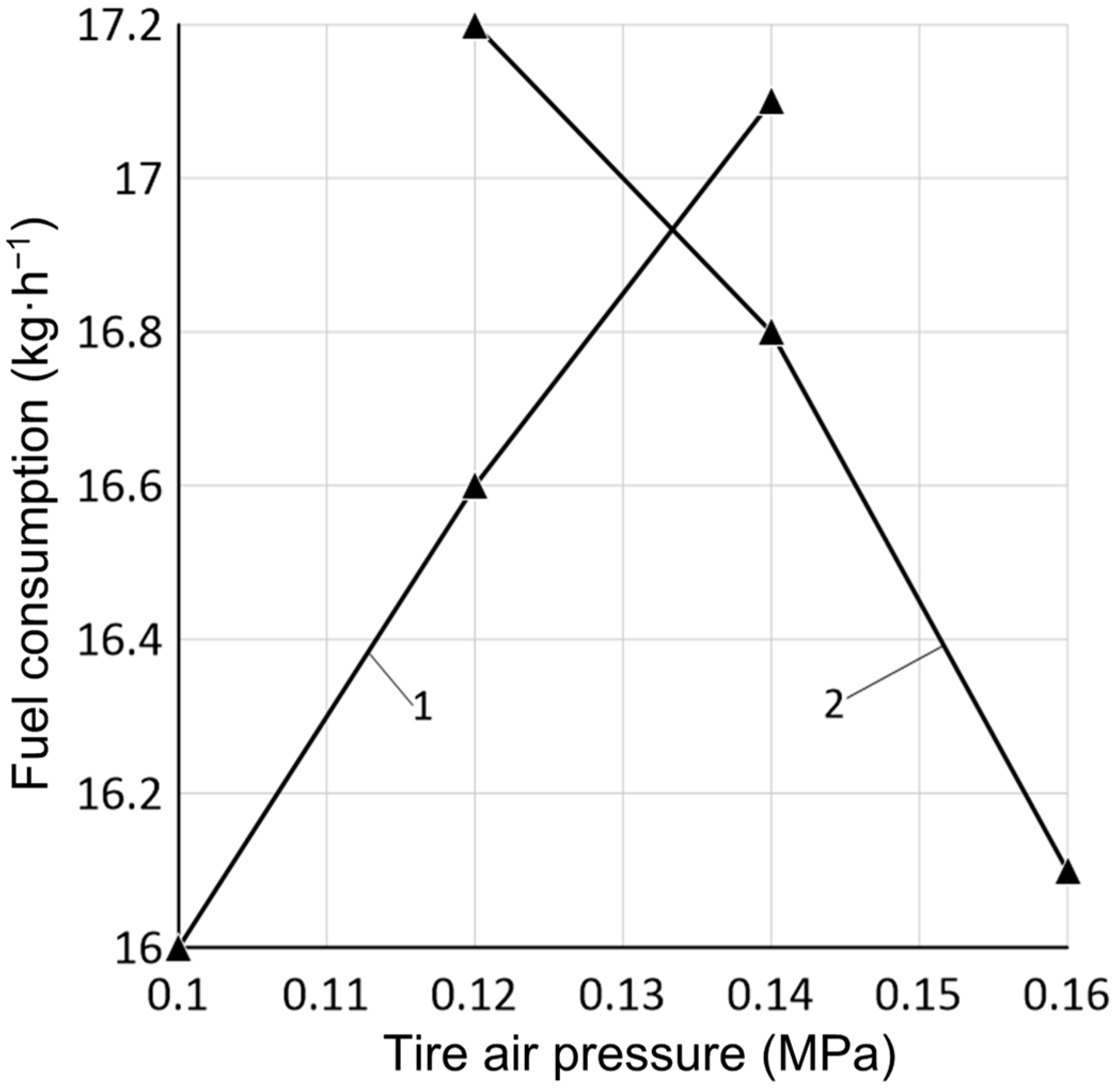
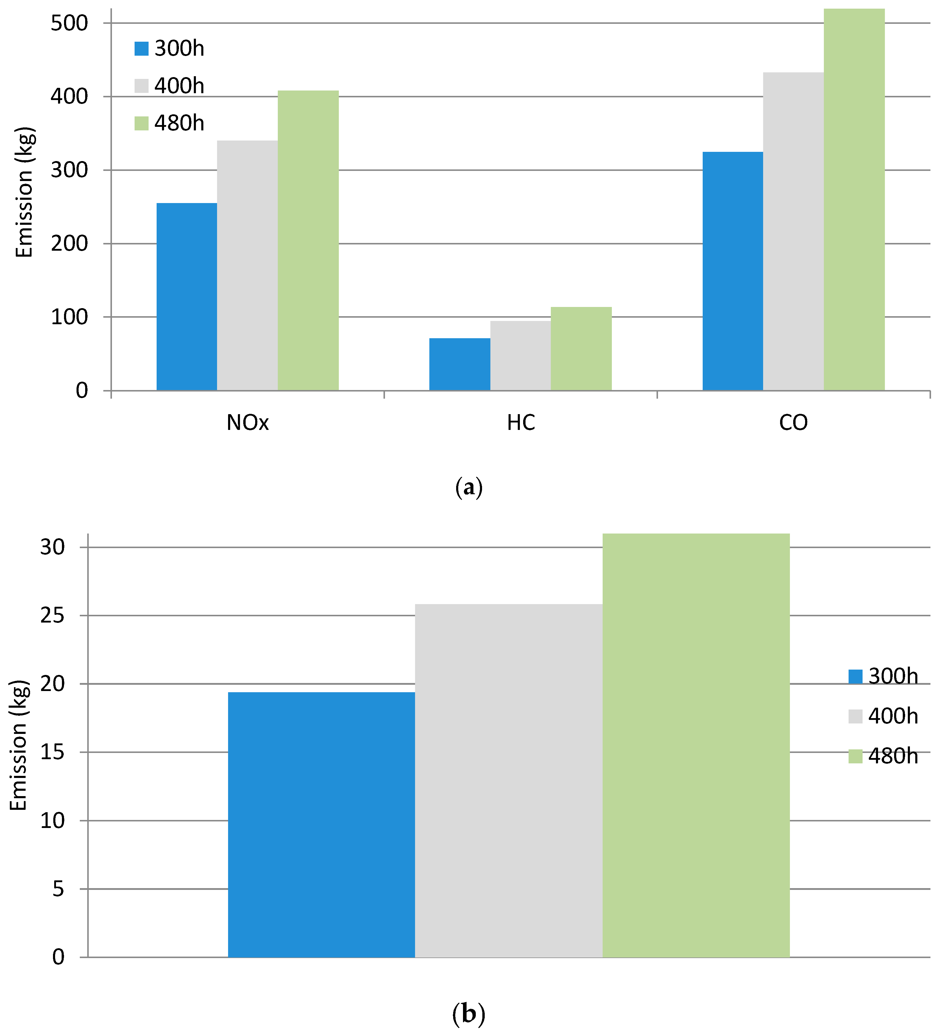
4. Results and Discussion

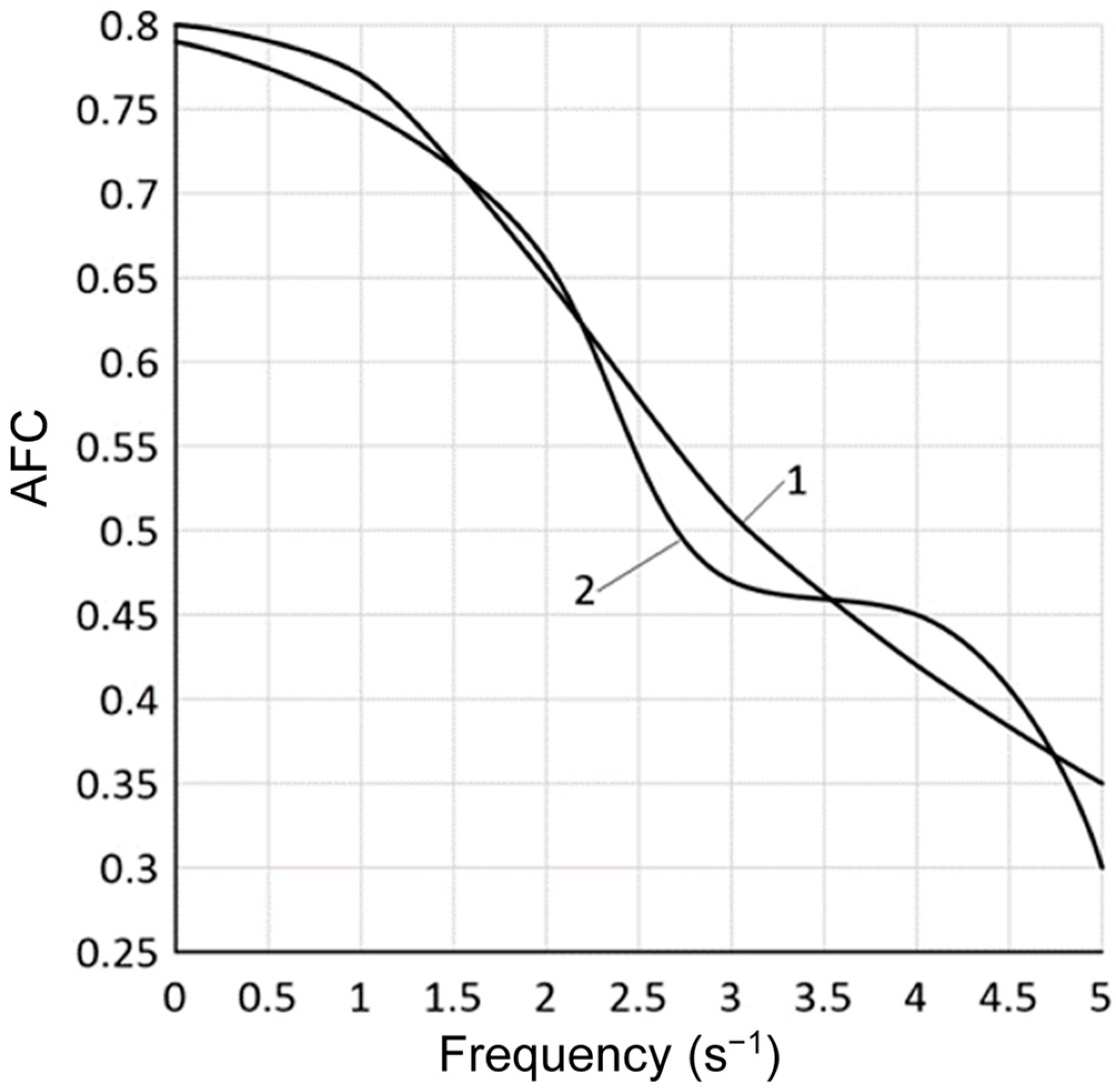
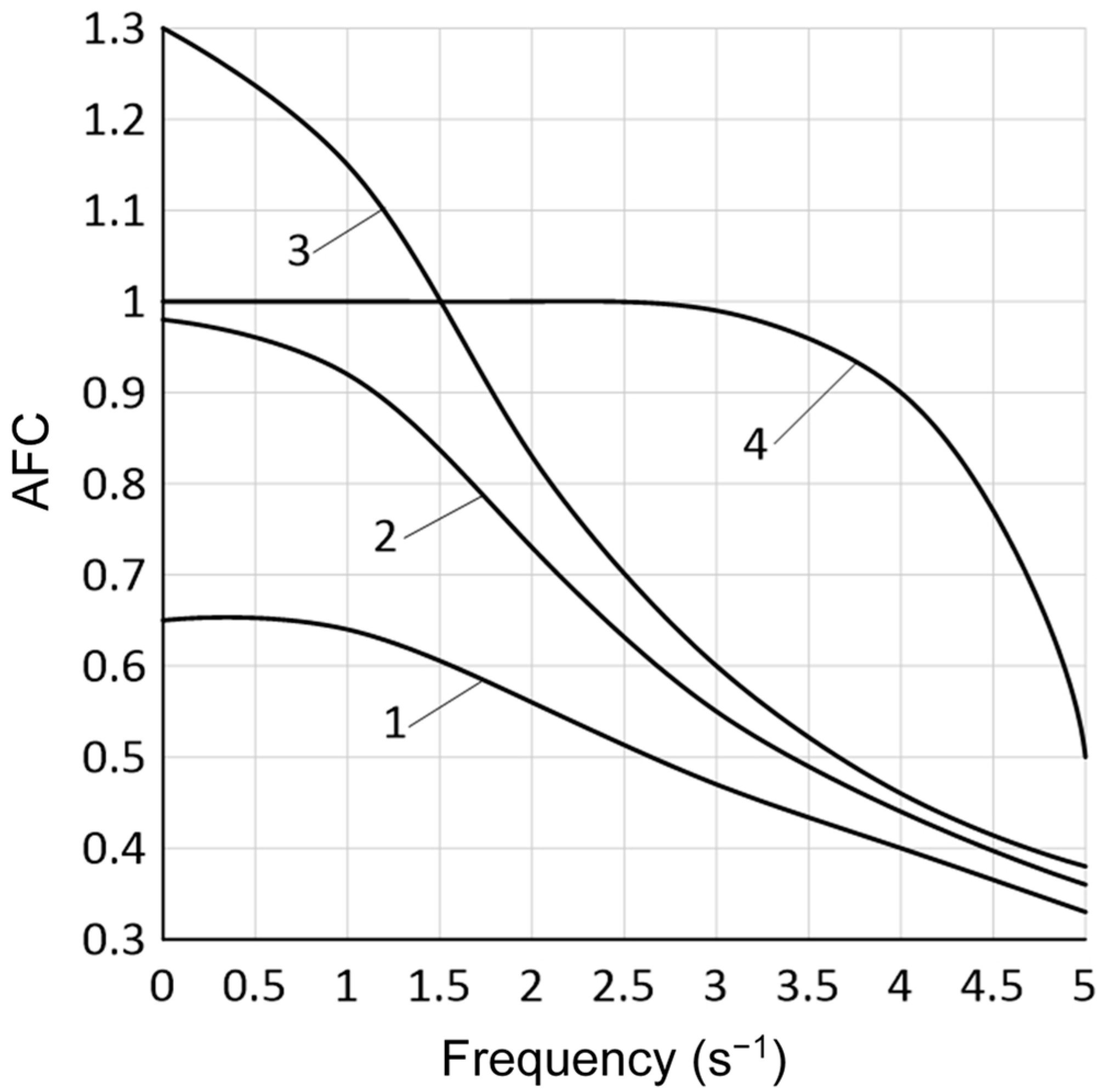
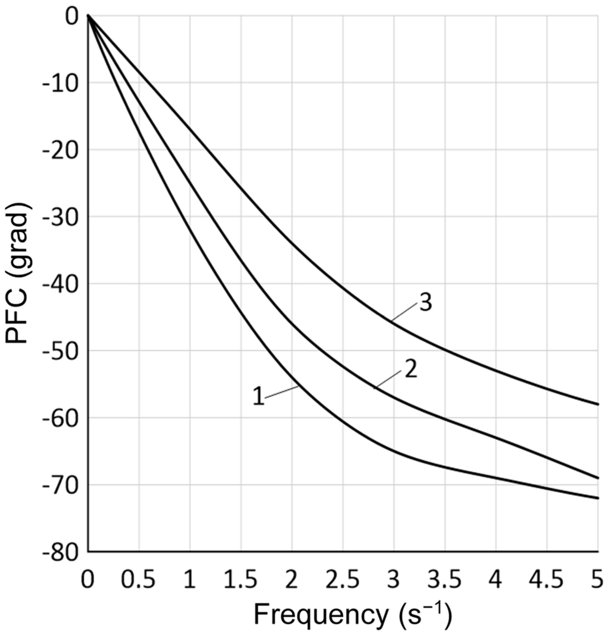
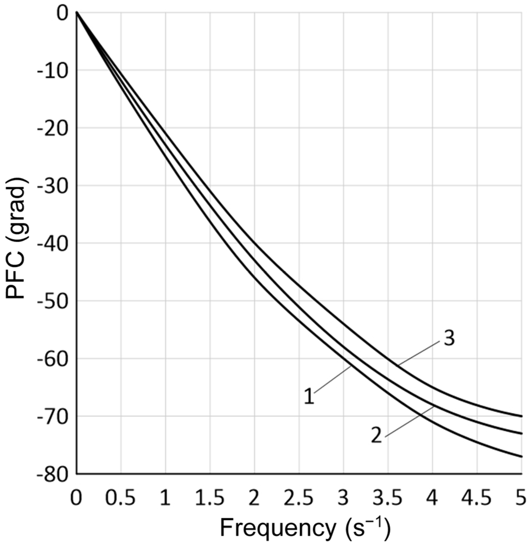
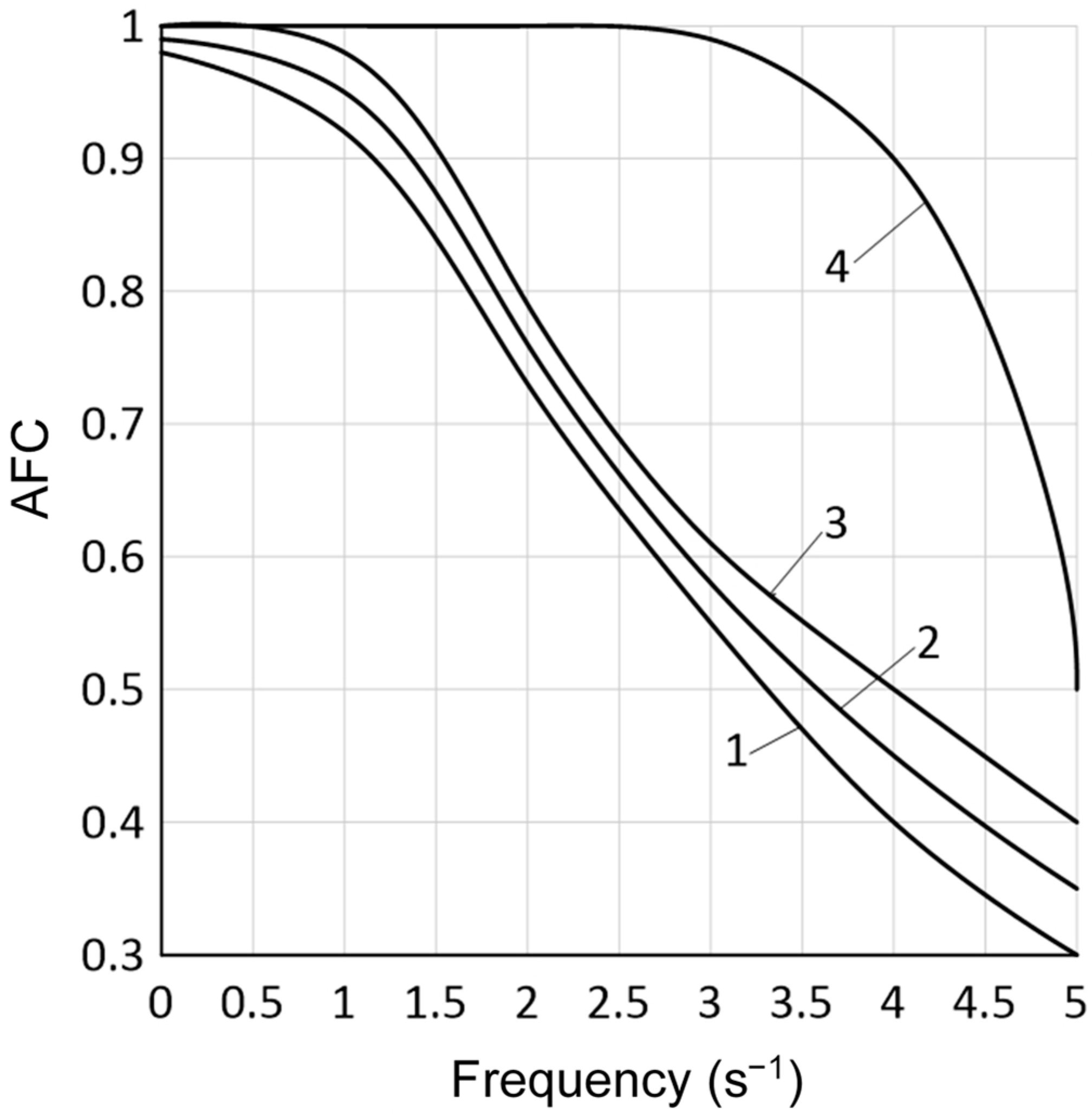
4.1. Checking the Mathematical Model for Adequacy

The conditions for conducting experimental studies of the harvesting unit are presented in

Table 1. Characteristics of the experimental winter wheat site.

Index	Value
Soil moisture in 0–10 cm layer (%)	14.2
Soil bulk density in the 0–10 cm (g·m−3) layer	1.26
Winter wheat yield (ton·ha−1)	4.08
Mean plant height (m)	0.68
Weed density (g·m−2)	16.8
Wheat stubble height (cm)	14.8
Stubble disc depth (cm)	8.6

.

As the analysis of experimental data showed, the oscillation spectrum of the tractor’s steered wheels’ rotation angle during the execution of the functional movement by the harvesting unit is of low-frequency (Figure 2). The main variance spectrum of this parameter is concentrated in the frequency range of 0–2 s⁻¹ (0–0.3 Hz), and its standard deviation is ±1.10 grad. The variance of the tractor’s heading angle oscillations is concentrated practically in the same frequency range (Figure 3). The standard fluctuation of this parameter is somewhat lower and is equal to 0.95 grad.

4.2. Results of Mathematical Modelling

Further calculation of the experimental AFC using Formula (3) and its comparison with the theoretical results showed that in almost the entire frequency range (0–5 s⁻¹) of the input signal oscillations (angle $\alpha$), the greatest discrepancy between the theoretical and experimental data does not exceed 10% (Figure 4). This result indicates the adequacy of the developed mathematical model, justifying its use for the reliable evaluation of the unit design and parameters for mowing agricultural crops while simultaneously chopping their stubble.

As a result of mathematical modelling, it was found that the nature of the control action determined by the dynamic system—in the form of the considered harvesting unit, along with the direct course of the tractor and the articulated conjunction of the disc harrow—depends on its velocity (Figure 5). As the value of $V_o$ approaches 3 m·s⁻¹ (curve 2), it more accurately responds to the control action. In the frequency interval of the latter 0–1 s⁻¹, the AFC of the harvesting unit is much closer to the perfect value (curve 4).

At the same time, at the velocity of its movement at the level of 4 m·s⁻¹ in the same frequency range of the angle $\alpha$ oscillations, there is an overshoot by the dynamic system of the control action. At a value of $\omega$ close to zero, the action (overshoot) reaches 30% (curve 3), which is an undesirable result.

However, we obtained unsatisfactory AFC at the velocity of the harvesting unit operating movement at the level of 2 m·s⁻¹ in the entire frequency range of the input signal (Figure 5, curve 1). Its nature indicates the presence of under-regulation in the dynamic system. This is manifested in the low accuracy of its response to the rotation angle of the tractor’s steered wheels.

The velocity of processing the input action by the dynamic system when changing the harvesting unit movement mode is characterized by its trend. Namely, an increase in the value of $V_o$ leads to a decrease in the reaction delay of the dynamic system to the tractor’s steered wheel rotation angle. Graphically, this is expressed in the rise of PFC in the entire range of these parameter fluctuations (Figure 6). But in quantitative terms, the growth of these phase-frequency characteristics is insignificant.

In connection with the above, in natural (field) operating conditions, it is advisable to keep the movement velocity of such a harvesting unit at a level of 3 m·s⁻¹. The intensity (frequency) of the impact on the tractor’s steering wheel should be as low as possible, within the range of 0–1 s⁻¹. As a result, as follows from the analysis of Figure 5 and Figure 6, with an acceptable delay, the dynamic system will respond accurately enough to the control action in the form of the steered wheel rotation angle of the self-propelled vehicle (in this case, the tractor).

Next, we consider the dependence of the considered unit movement controllability on the resistance coefficients to the yaw of the tractor’s front and rear tyres ($k_a$ and $k_b$). Their values were calculated from the equation in Ref. [46]:

$$\begin{array}{c}{k}_a\left(k_b\right)=145·\left[1.75{\displaystyle \frac{h}{D}}-12.7{\left({\displaystyle \frac{h}{D}}\right)}^2\right]·{\rho }_w·b^2\end{array}$$

(4)

where $h$—track depth after tractor passing, m; $D,b$—diameter of the wheel and the width of its tyres respectively, m; ${\rho }_w$—tyre air pressure, MPa.

The analysis of dependence (4) shows that practically the only parameter whose change does not affect the tractor’s design is ${\rho }_w$. For the tractor’s rear wheels, the value of this parameter was taken to equal 0.10, 0.12, and 0.14 MPa. These pressures corresponded to the following values of the coefficient $k_b$: 66, 80, and 94 kN·rad⁻¹.

Calculations have established that the effect of changing the air pressure in the tractor’s rear wheel tyres (and hence, the coefficient $k_b$) on the AFC determined by the considered dynamic control system depends on its frequency. At $\omega$ = 0–1.5 s⁻¹; an increase in the value of $k_b$ causes a decrease in the corresponding AFCs (Figure 7). Theoretically, this indicates a deterioration in the harvesting unit movement controllability.

The opposite situation occurs for the rotation angle oscillation frequency of the tractor’s steered wheels ω > 1.5 s⁻¹. Namely, an increase in the value of $k_b$ leads to a slight but desirable increase in the amplitude–frequency characteristics.

The phase shift behaves quite unambiguously over the entire range of the input action oscillation frequency (the tractor’s steered wheel rotation angle). Increasing the yaw coefficient value of the tractor’s rear wheels contributes to the desired reduction (i.e., lift) of the respective PFCs (Figure 8).

The air pressure in the tractor’s front wheel tyres was changed from 0.12 to 0.16 MPa. This corresponded to the values of the yaw resistance coefficient $k_a$ ranging 99 to 131 kN·rad⁻¹. Calculations have established that increasing this parameter improves the controllability of the movement of the harvesting unit. In the range of the angle $\alpha$ oscillation frequencies 0–1 s⁻¹ at $k_a$ = 131 kN·rad⁻¹, the AFC of the dynamic system, when it processes the input signal, is generally close to perfect (curve 3, Figure 9).

Let us consider how the results of theoretical studies on the controllability of the movement of the harvesting unit are consistent with its fuel energy consumption. It has been experimentally established that setting the air pressure in the tractor’s rear tyres to 0.14 and even 0.12 MPa reduces the controllability of the harvesting unit. To track the trajectory of its previous pass, in this case, the driver, was forced to increase the steering wheel speed to 2.0 s⁻¹. When the harvesting unit travelled with an air pressure of 0.10 MPa in the rear tractor tyres, the steering wheel rotation speed did not exceed 1.0 s⁻¹.

As a result, an increase in the air pressure in the tyres of the unit’s rear wheels led to an increase in hourly fuel consumption (curve 1, Figure 10). When the value of the ${\rho }_w$ parameter changed from 0.10 to 0.14 MPa, this increase amounted to 1.10 kg·h⁻¹, which is equivalent to an increase in energy of 50.5 MJ·h⁻¹, or 6.8%.

We noted above that the air pressure in the tyre determines the value of its yaw resistance coefficient. It follows that to improve motion controllability and reduce energy consumption by the harvesting unit, it is advisable to set the value of the $k_b$ parameter lower. As noted above, in practice, this is realized by setting a lower air pressure in the tractor’s rear wheel tyres.

When changing the air pressure in the tractor’s front wheel tyres, a diametrically opposite result was obtained. Namely, an increase in the ${\rho }_w$ parameter from 0.12 to 0.16 MPa led to an improvement in the controllability of the harvesting unit. This was manifested in a reduction in the driver’s steering wheel speed from 1.90 to 0.95 s⁻¹. At the same time, the unit’s fuel consumption decreased from 17.20 to 16.05 kg·h⁻¹ (curve 2, Figure 10). Regarding energy consumption, the reduction is 57.5 MJ·h⁻¹, or 6.7%.

Considering the above relationship between the air pressure in the tyres and the coefficient of resistance to its yaw ($k_a$), it is advisable to set the ka parameter value higher to improve the movement controllability and reduce the energy consumption of the harvesting unit.

Considering the above relationship between the air pressure in the tyres and the coefficient of resistance to its yaw ($k_a$), it is advisable to set the ka parameter value large to improve the movement controllability and reduce the energy consumption of the harvesting unit.

In order to build a generalised model, a measurement decomposition table was used (

Table 2. Characteristics of the pressure measurements.

No.	pa	pb	Measurement
1	1	1	17.3
2	1	2	17.1
3	2	1	16.05
4	2	2	16.8

).

Where: $p_a=1$—the minimum value of tyre pressure in the front wheels adopted in experimental tests, i.e., 0.12 MPa; $p_a=2$—the maximum value of tyre pressure in the front wheels adopted in the tests, i.e., 0.16 MPa, $p_b=1$—the minimum value of tyre pressure in the rear wheels adopted in experimental tests, i.e., 0.1 MPa; $p_b=2$—the maximum value of tyre pressure in the rear wheels adopted in the tests, i.e., 0.14 MPa. The grand average was $y_{avg}=16.81$.

The linear model showing the influence of tyre pressure on fuel consumption, determined on the basis of the experimental data, is as follows:

$$y\left(p_a,p_b\right)=16.81+p_a\left[\begin{array}{c}0.39\\ -0.39\end{array}\right]+p_b\left[\begin{array}{c}-0.14\\ 0.14\end{array}\right]+p_a{p}_b\left[\begin{array}{cc}0.24& -0.24\\ -0.23& 0.24\end{array}\right]$$

(5)

where: $p_a$—tyre pressure in the front wheels; $p_b$—tyre pressure in the rear wheels. The $y\left(p_a,p_b\right)$unit is $\left[{\displaystyle \frac{\mathrm{k}\mathrm{g}}{\mathrm{h}}}\right]$.

Using the harvesting unit’s carbon footprint calculator, the carbon footprint values were calculated for variable fuel consumption values, leaving the remaining values the same. The results show that reducing the pressure from 0.14 MPa to 0.1 MPa in the rear tyres reduces the carbon footprint by 4.2 kg CO₂ eq/h. However, increasing the pressure in the front tyres also reduces the carbon footprint by 4.2 kg CO₂ eq/h.

Then, calculations were performed for the exhaust emission of the HTZ-16131 tractor powered by the BF6M1013E engine, with a maximum power of 137 kW (

Table 3. Technical data for the engine of the tested tractor.

Tested Object (BF6M1013E)	Parameter
Stroke (travel) volume [dm3]	7.2
Number and arrangement of cylinders [–]	6, inline
Maximum power [kW]	137 at 2300 rpm
Maximum torque [Nm]	720 at 1400 rpm
Exhaust gas treatment systems	DOC
Homologation standard	Stage II

). The methods for calculating emissions for agricultural machinery, in accordance with the Tier 2 and Tier 3 methodology, which include fuel consumption, engine power, operating time, and emission factors, are presented below in

Table 4. Overview of EU directive requirements relevant for control of emissions from diesel-fuelled non-road machinery.

Stage II	Engine Size [kW]	CO [g/kWh]	VOC [g/kWh]	NOx [g/kWh]	VOC + NOx [g/kWh]	PM [g/kWh]	Tractors
							EU Directive	Implement. Date
E	$130\le \mathrm{P}<560$	3.5	1	6	-	0.2	2000/25	1/7 2002

,

Table 5. Tier 2 emission factors.

Fuel	NFR Sector	Pollutant	Units	Technology Stage II
Diesel	Agriculture	BC	g/ton fuel	482
		CH4	g/ton fuel	29
		CO	g/ton fuel	6104
		CO2	g/ton fuel	3160
		N2O	g/ton fuel	138
		NH3	g/ton fuel	8
		NMVOC	g/ton fuel	1181
		NOx	g/ton fuel	20,612
		PM10	g/ton fuel	624
		PM2.5	g/ton fuel	624
		TSP	g/ton fuel	624

,

Table 6. Baseline emission factors and fuel consumption (FC) for diesel NRMM [g/kWh].

Engine Power (kW)	Technology Level	NOx	VOC	CH4	CO	N2O	NH3	PM	PM10	PM2.5	BC	FC
$130\le \mathrm{P}<560$	Stage II	5.2	0.3	0.007	1.5	0.035	0.002	0.1	0.1	0.1	0.07	250
	Stage V	0.4	0.13	0.003	1.5	0.035	0.002	0.015	0.015	0.015	0.002	250

,

Table 7. Deterioration factors for diesel machinery relative to average engine life time.

Emission Level	NOx	VOC	CO	TSP
Stage II	0.009	0.034	0.101	0.473
Stage IIIA, IIIB, IV, V	0.008	0.027	0.151	0.473

and

Table 8. Transient operation adjustment factors for diesel engines in non-road machines.

Technology Level	Load	Load Factor	NOx	VOC	CO	TSP	FC
Stage II and prior	High	>0.45	0.95	1.05	1.53	1.23	1.01
	Middle	0.25 ≤ LF < 0.45	1.025	1.67	2.05	1.6	1.095
	Low	<0.25	1.1	2.29	2.57	1.97	1.18

[57].

In order to theoretically determine exhaust emission depending on the type of fuel and the level of engine production technology.

The generic algorithm for calculating emissions for agriculture machinery using the Tier 2 methodology, as suggested in Ref. [57], is as follows:

$${\mathrm{E}}_i=\sum _j\sum _t\mathrm{F}{\mathrm{C}}_{j,t}\times \mathrm{E}{\mathrm{F}}_{i,j,t}$$

(6)

where: ${\mathrm{E}}_i—$mass of emissions of pollutant “i” during the inventory period; $\mathrm{F}{\mathrm{C}}_{j,t}$—fuel consumption of fuel type “j” by equipment category C and of technology type “t”; $\mathrm{E}{\mathrm{F}}_{i,j,t}$—average emission factor for pollutant “i” for fuel type “j” for equipment category C and of technology type “t”. $i$—pollutant type; j—fuel type (diesel); t—off-road equipment technology (Stage II).

In essence, this involves subdividing the diesel consumption, as fuel type j, used by the NFR sectors in the second summation in the (1) algorithm, is equal to the single term, i.e.,

$$\sum _t\mathrm{F}{\mathrm{C}}_{j,t}=\mathrm{F}{\mathrm{C}}_j$$

(7)

The Tier 2 methods outlined in the section above uses fuel statistics, multiplied by technology-specific emission factors. However, this method can be difficult to undertake because fuel consumption data are often not available at the required level of detail. Therefore, in this study, more detailed Tier 3 methodology is employed. This methodology uses hours of operation as the main activity data and is primarily based on the US-EPA method for estimating off-road emissions (US-EPA 1991). The Tier 3 method presented here has been updated and includes detailed fuel consumption and emission information taken, to a large extent, from the German TREMOD NRMM model.

The algorithm used in the Tier 3 methodology is as follows:

$$\mathrm{E}=\mathrm{N}\times \mathrm{H}\mathrm{R}\mathrm{S}\times \mathrm{P}\times (1+\mathrm{D}\mathrm{F}\mathrm{A})\times \mathrm{L}\mathrm{F}\mathrm{A}\times \mathrm{E}{\mathrm{F}}_{\mathrm{B}\mathrm{a}\mathrm{s}\mathrm{e}}$$

(8)

where: $\mathrm{E}$—mass of emissions of pollutant “i” during the inventory period; $\mathrm{N}$—number of engines (units); $\mathrm{H}\mathrm{R}\mathrm{S}$—annual hours of use; $\mathrm{P}$—engine size (kW); $\mathrm{D}\mathrm{F}\mathrm{A}$—deterioration factor adjustment; $\mathrm{L}\mathrm{F}\mathrm{A}$—load factor adjustment; $\mathrm{E}{\mathrm{F}}_{\mathrm{B}\mathrm{a}\mathrm{s}\mathrm{e}}$—base emission factor (g/kWh) (this is, for each pollutant, a function of the technology levels and the power output).

Up to Stage II: The EFs for fuel consumption and NO_x, VOC, CO, and TSP emissions for technology levels up to and including Stage II are reported in the TREMOD NRMM model (IFEU 2004). These are based on measured data from a range of different studies and data suggested from literature reviews [58].

Deterioration factor adjustments for diesel (DFA):

$$D{F}_D={\displaystyle \frac{K}{LT}}D{F}_{y,z}$$

(9)

where K—engine age (between 0 and average life time); LT—average lifetime; y—engine-size class; z—technology level.

The load adjustment factors are presented in Table 8.

The diesel fuel recommended by the manufacturer, HTZ-16131, with a BF6M1013E engine (technical data is presented in Table 3) was used for the tests, i.e., GOST 305-82 class L with a sulphur mass fraction of up to 0.2%.

Table 9. Physicochemical properties of diesel fuel GOST 305-82 (2013) class L.

Indicator Name	Value for GOST 305-82, Class L
Cetane number not less than:	45
Factional composition: Up to 50% is distilled at a temperature of °C, not higher than: A total of 95% is distilled at a temperature of °C, not higher than:	280 360
Kinematic viscosity at 20° (mm2/s):	3.0–6.0
Mass fraction of sulphur, %, not more than: Type I Type II	0.2 0.05
The actual soot concentration in mg per 100 cm3 of fuel, not more than:	40
mg KOH per 100 cm3 of fuel, not more than:	5
Iodine number, g of iodine per 100 g of fuel, not more than:	6
Residue after incineration [%], not more than:	0.01
Degree of coking, 10% residue, %, not more than:	0.20
Filterability factor, not more than:	3
Density at 20 °C, kg/m3, not more than:	860
Ignition point [°C]:	56
Water content:	No data available

below presents the most important parameters of diesel oil.

Due to the low environmental class of diesel oil GOST 305-82 (2013)—K2, verva-on premium diesel oil (class B0) was also used for testing (

Table 10. Physical and chemical properties of diesel oil: verva-on premium (class B0), provided by the manufacturer, and results of laboratory tests of the second fuel used for exhaust emission tests of the harvesting unit, carried out in accordance with the methodology described in the relevant standards [59,60,61,62,63,64,65,66,67,68,69,70].

Indicator Name	Verva-on Premium (Class B0)	GOST 305-82 (Class L)
Cetane number not less than:	52.6 (test method PN-EN ISO 5165)	51 (test method PN-EN ISO 5165)
Factional composition: Up to 65% is distilled at a temperature of °C, not higher than: minimum 5% to a temperature of °C: 95% is distilled to a temperature of °C:	250 350 (test method PN-EN ISO 3405) Max. 360	250 350 (test method PN-EN ISO 3405) Max. 360
Kinematic viscosity at 40° (mm2/s):	2.0–4.5 (test method PN-EN ISO 3104)	2.15 (test method PN-EN ISO 3104)
Sulphur content [mg/kg]:	Max. 10 (test method as per PN-EN ISO 20846, PN-EN ISO 20884)	8.8 (test method as per PN-EN ISO 20846, PN-EN ISO 20884)
Residue after incineration [%], not more than:	0.01 (test method PN-EN ISO 6245)	0.01 (test method PN-EN ISO 6245)
Residue after coking in 10% of the distilled residue:	0.30 (test method PN-EN ISO 10370)	0.27 (test method PN-EN ISO 10370)
Density at 15 °C, kg/m3:	820–845 (test method as per PN-EN ISO 12185, PN-EN ISO 3675)	833.6 (test method as per PN-EN ISO 12185, PN-EN ISO 3675)
Ignition temperature [°C]:	Minimum 56 (test method PN-EN ISO 2719)	61 (test method PN-EN ISO 2719)
Water content mg/kg/%:	Max. 200/0.02 (test method PN-EN ISO 12937)	22 (test method PN-EN ISO 12937)

).

Using the Tier 2 model, the exhaust gas emission coefficients were calculated for individual values of fuel consumption experimentally measured under actual operating conditions of the harvesting unit. Then, the decrease in emissivity for the individual harmful substances due to energy savings related to the change in the pressure in the tyres of the harvesting unit’s road wheels was calculated, which is presented in the graph in Figure 11. Additionally, the impact of the type of diesel fuel burned on the change in the emissivity of the harvesting unit was also examined. The suggestion that changing the diesel fuel resulted in an additional reduction in fuel consumption by approximately 3.5% was also experimentally tested. This change is directly related to the physicochemical properties of diesel fuels, mainly the cetane number and the ignition temperature.

Using the model included in the standard in Ref. [57], the emission intensity coefficients of selected harmful substances was determined in kilograms per year.

It should be emphasized that in accordance with the operational life of agricultural tractors, their annual hourly working time is approximately 480 h. By performing two agrotechnical operations during one tractor run, we are able to reduce the annual working time by up to 180 h (assuming the distance of equipment storage from the workplace to be 1 km and a large area of the cultivated field).

Figure 12 shows that the use of an agricultural unit in the form of the analysed harvesting unit reduces the annual emission of particulate matter (PM) by as much as 11.624 kg (Figure 12b), while reducing the annual number of working hours from 480 to 300. When the annual hourly working time is reduced by 80 h, then the emission of particulate matter in the exhaust gases will decrease by 5.166 kg. A high emission reduction value was achieved, i.e., carbon monoxide (CO) by 194.806 kg; NO_x by 153.024 kg (Figure 12a). It should be emphasized that the determined values do not take into account fuel consumption under the given operating conditions and the physicochemical properties of burned diesel oil. They are determined based on the power of the driving unit, the number of operating hours per year, and the level of technology at which the power supply unit was manufactured. Therefore, based on the Tier 2 model, the value in kilograms of annual particulate matter (PM) emissions was calculated for 300, 400, and 480 h of operation per year, respectively, assuming the lowest experimentally obtained fuel consumption and the use of Verva-on Premium diesel oil. The results are presented in Figure 13.

5. Conclusions

In this article, optimisation was performed to minimise fuel consumption while maintaining maximum controllability of the analysed harvest unit. Reduced rear tyre pressure and increased front tyre pressure have been experimentally proven to reduce fuel consumption by 1.1 kg·h⁻¹, on average. On the basis of experimental data obtained under field conditions, a linear model of the effect of tyre pressure on fuel consumption was constructed. In addition, a harvesting unit carrying out two agrotechnical processes during a single tractor run reduces the hourly annual working time by up to 180 h (assuming the storage distance of the equipment from the workplace to be up to 1 km and a large arable field area). It has been experimentally proven that a change in diesel fuel resulted in an additional reduction in fuel consumption of about 3.5%. This change is directly related to the physicochemical properties of diesel oils, mainly the cetane number and the ignition temperature. It has been shown that by reducing the annual number of working hours resulting from the use of the harvesting unit, the annual emissions of particulate matter (PM) are reduced by 11.624 kg, i.e., carbon monoxide (CO) by 194.806 kg and NO_x by 153.024 kg.

References

1. Santeramo, F.G.; Kang, M. Food Security Threats and Policy Responses in EU and Africa. Sustain. Horiz. 2022, 4, 100044. [Google Scholar] [CrossRef]
2. Ranta, R.; Mulrooney, H. Pandemics, food (in)security, and leaving the EU: What does the COVID-19 pandemic tell us about food insecurity and Brexit. Soc. Sci. Humanit. Open 2021, 3, 100125. [Google Scholar] [CrossRef]
3. Granato, D.; Zabetakis, I.; Koidis, A. Sustainability, nutrition, and scientific advances of functional foods under the new EU and global legislation initiatives. J. Funct. Foods 2023, 109, 105793. [Google Scholar] [CrossRef]
4. Saboori, B.; Alhattali, N.A.; Gibreel, T. Agricultural products diversification-food security nexus in the GCC countries; introducing a new index. J. Agric. Food Res. 2023, 12, 100592. [Google Scholar] [CrossRef]
5. European Parliament Resolution of 13 December 2022 on a Long-Term Vision for EU Rural Areas—Towards Stronger, Better Connected, Resilient and Prosperous Rural Areas by 2040 (2021/2254(INI)). Available online: https://www.prawo.pl/akty/dz-u-ue-c-2023-177-35,72165028.html (accessed on 26 September 2023).
6. Farms and Farmland in the European Union—Statistics. Available online: https://ec.europa.eu/eurostat/statistics-explained/SEPDF/cache/73319.pdf (accessed on 26 September 2023).
7. New Report Highlights Biomethane Ramp-up and Best Pathways for Full Renewable Gas Deployment. Available online: https://www.europeanbiogas.eu/new-report-highlights-biomethane-ramp-up-and-best-pathways-for-full-renewable-gas-deployment/ (accessed on 26 September 2023).
8. Hughes, H.M.; Koolen, S.; Kuhnert, M.; Baggs, E.M.; Maund, S.; Mullier, G.W.; Hillier, J. Towards a farmer-feasible soil health assessment that is globally applicable. J. Environ. Manag. 2023, 345, 118582. [Google Scholar] [CrossRef] [PubMed]
9. Bocci, R.; Bussi, B.; Petitti, M.; Franciolini, R.; Altavilla, V.; Galluzzi, G.; Luzio, P.; Migliorini, P.; Spagnolo, S.; Floriddia, R.; et al. Yield, yield stability and farmers’ preferences of evolutionary populations of bread wheat: A dynamic solution to climate change. Eur. J. Agron. 2020, 121, 126156. [Google Scholar] [CrossRef]
10. Akimowicz, M.; Corso, J.P.; Gallai, N.; Képhaliacos, C. Adopt to adapt? Farmers’ varietal innovation adoption in a context of climate change. The case of sunflower hybrids in France. J. Clean. Prod. 2021, 279, 123654. [Google Scholar] [CrossRef]
11. Beitnes, S.S.; Kopainsky, B.; Potthoff, K. Climate change adaptation processes seen through a resilience lens: Norwegian farmers’ handling of the dry summer of 2018. Environ. Sci. Policy 2022, 133, 146–154. [Google Scholar] [CrossRef]
12. Castellari, E.; Soregaroli, C.; Venus, T.J.; Wesseler, J. Food processor and retailer non-GMO standards in the US and EU and the driving role of regulations. Food Policy 2018, 78, 26–37. [Google Scholar] [CrossRef]
13. Eriksson, D.; Custers, R.; Björnberg, K.E.; Hansson, S.O.; Purnhagen, K.; Qaim, M.; Romeis, J.; Schiemann, J.; Schleissing, S.; Tosun, J.; et al. Options to Reform the European Union Legislation on GMOs: Post-authorization and Beyond. Trends Biotechnol. 2020, 38, 465–467. [Google Scholar] [CrossRef]
14. CEMA. Report. European Agricultural Machinery Industry. Available online: https://www.cema-agri.org/images/publications/brochures/CEMA_Industry_Report_2022-.pdf (accessed on 26 September 2023).
15. Anastasiou, E.; Fountas, S.; Voulgaraki, M.; Psiroukis, V.; Koutsiaras, M.; Kriezi, O.; Lazarou, E.; Vatsanidou, A.; Fu, L.; Bartolo, F.; et al. Precision farming technologies for crop protection: A meta-analysis. Smart Agric. Technol. 2023, 5, 100323. [Google Scholar] [CrossRef]
16. Krisnawijaya, N.N.K.; Tekinerdogan, B.; Catal, C.; Tol, R. Multi-Criteria decision analysis approach for selecting feasible data analytics platforms for precision farming. Comput. Electron. Agric. 2023, 209, 107869. [Google Scholar] [CrossRef]
17. Sharma, V.; Tripathi, A.K.; Mittal, H. Technological revolutions in smart farming: Current trends, challenges & future directions. Comput. Electron. Agric. 2022, 201, 107217. [Google Scholar] [CrossRef]
18. Kostencki, P.; Stawicki, T.; Królicka, A. Wear of the working parts of agricultural tools in the context of the mass of chemical elements introduced into soil during its cultivation. Int. Soil Water Conserv. Res. 2021, 9, 229–240. [Google Scholar] [CrossRef]
19. Herrera, H.; Schütz, L.; Paas, W.; Reidsma, P.; Kopainsky, B. Understanding resilience of farming systems: Insights from system dynamics modelling for an arable farming system in the Netherlands. Ecol. Model. 2022, 464, 109848. [Google Scholar] [CrossRef]
20. Biagini, L.; Antonioli, F.; Severini, S. The impact of CAP subsidies on the productivity of cereal farms in six European countries: A historical perspective (2008–2018). Food Policy 2023, 119, 102473. [Google Scholar] [CrossRef]
21. Wu, C.; Xiao, S.; Jin, M. Comparation on rape combine harvesting and two-stage harvesting. Trans. Chin. Soc. Agric. Eng. 2014, 30, 10–16. [Google Scholar]
22. Rudoy, D.; Egyan, M.; Kulikova, N.; Chigvintsev, V. Review and analysis of technologies for harvesting perennial grain crops. IOP Conf. Ser. Earth Environ. Sci. 2021, 937, 022112. [Google Scholar] [CrossRef]
23. Bulgakov, V.; Nadykto, V.; Kaletnik, H.; Ivanovs, S. Field experimental investigations of performance and technological indicators of operation of swath header asymmetric machine-and-tractor aggregate. Eng. Rural Dev. 2018, 17, 227–233. Available online: https://www.tf.lbtu.lv/conference/proceedings2018/Papers/N269.pdf (accessed on 26 September 2023). [CrossRef]
24. Konstantinov, K.; Gluchkov, I.; Ognev, I. Justification Optimal Operating Parameters of the Conveyor, Which Is the Mechanism of the Header for Two–Phase Harvesting by Batch Method, Taking into Account the Minimization of Losses of Grain. Available online: https://www.e3s-conferences.org/articles/e3sconf/pdf/2019/52/e3sconf_icmtmte2019_00046.pdf (accessed on 26 September 2023).
25. Alfalfa Management Guide. Available online: https://www.agronomy.org/files/publications/alfalfa-management-guide.pdf (accessed on 26 September 2023).
26. Bulgakov, V.; Pascuzzi, S.; Nadykto, V.; Ivanovs, S. A Mathematical Model of the Plane-Parallel Movement of an Asymmetric Machine-and-Tractor Aggregate. Agriculture 2018, 8, 151. [Google Scholar] [CrossRef]
27. Bulgakov, V.; Nadykto, V.; Ivanovs, S.; Nowak, J. Research of variants to improve steerability of movement of trailed asymmetric harvesting aggregate. Eng. Rural Dev. 2019, 18, 136–143. Available online: https://www.tf.lbtu.lv/conference/proceedings2019/Papers/N169.pdf (accessed on 26 September 2023). [CrossRef]
28. Shu, C.; Lei, Y.; Lei, L.; Han, C.; Jiang, Y.; Ding, Y.; Liao, Q. Pipeline Design and Simulation Optimization of Hydraulic Driving System for Rape Windrower. J. Syst. Simul. 2015, 27, 3087–3095. [Google Scholar]
29. Foster, A.A.; Strosser, R.P.; Peters, J.; Sun, J.-Q. Automatic velocity control of a self-propelled windrower. Comput. Electron. Agric. 2005, 47, 41–58. [Google Scholar] [CrossRef]
30. Gesce, D.M. New windrower series added to Hesston lineup. Diesel Prog. N. Am. Ed. 2004, 70, 76–77. [Google Scholar]
31. Li, J.; Zhao, J.; Liu, S.; Hou, X.; Chen, X.; Zhang, X. Design and Experiment of Self-propelled Pea Windrower. Trans. Chin. Soc. Agric. Mach. 2021, 52, 107–116. [Google Scholar]
32. Jin, M.; Zhang, M.; Wang, G.; Liang, S.; Wu, C.; He, R. Analysis and Simulation of Wheel-Track High Clearance Chassis of Rape Windrower. Agriculture 2022, 12, 1150. [Google Scholar] [CrossRef]
33. Shinners, T.J.; Digman, M.F.; Panuska, J.C. Overlap loss of manually and automatically guided mowers. Appl. Eng. Agric. 2012, 28, 5–8. [Google Scholar] [CrossRef]
34. Roper, M.M.; Ward, P.R.; Keulen, A.F.; Hill, J.R. Under no-tillage and stubble retention, soil water content and crop growth are poorly related to soil water repellency. Soil Tillage Res. 2013, 126, 143–150. [Google Scholar] [CrossRef]
35. Konstantinov, M.; Glushkov, I.; Mukhamedov, V.; Lovchikov, A. Increase in Soil Moisture Reserves due to the Formation of High Stubble Residues for the Accumulation of Snow Precipitation. Available online: https://iopscience.iop.org/article/10.1088/1755-1315/666/5/052049/pdf (accessed on 26 September 2023).
36. Tsibulka, N.N.; Youkhnovets, A.V.; Tzhukova, I.I. Influence of Mechanical Processing Methods and Techniques on the Soil Dynamics Moisture. Bull. MDU Named After A.A. Kulyashova 2005, 1, 111–119. Available online: https://libr.msu.by/bitstream/123456789/14389/1/5414n.pdf (accessed on 26 September 2023).
37. Nosalewicz, A.; Kuś, J.; Lipiec, J. Effect of tillage methods on soil penetration resistance. Acta Agrophysica 2009, 14, 675–682. [Google Scholar]
38. Pabin, J. Cultivation of the Role and Physical Properties of the Soil and the Yielding of Plants. Available online: https://iung.pl/sir/zeszyt08_13.pdf (accessed on 10 July 2024).
39. Buliński, J.; Sergiel, L. Soil considerations in cultivation of plants. Ann. Wars. Univ. Life Sci.-SGGW Agric. 2013, 61, 5–15. [Google Scholar]
40. Magnuszewski, A.; Soczyńska, U. International Hydrological Dictionary, 1st ed.; Wydawnictwo Naukowe PWN (Państwowe Wydawnictwo Naukowe): Warszawa, Poland, 2001; pp. 1–250. [Google Scholar]
41. Pabin, J.; Włodek, S.; Biskupski, A. Water Content in Different Agrosystems. Ecol. Chem. Eng. 2003, 10, 319–325. [Google Scholar]
42. Gąsior, J.; Kaniuczek, J.; Hajduk, E.; Właśniewski, S.; Nazarkiewicz, M.; Bilek, M. Methods of studying the physical properties of soils. Acta Carpathica 2013, 6, 43–50. [Google Scholar]
43. Maslov, G.; Remizov, I.; Semyakov, G.; Karakai, I. Harvesting and soil-cultivating unit based on the TORUM combine. Mach. Equip. Village 2010, 2, 18–19. [Google Scholar]
44. Average Area of Agricultural Land on the Holding in 2023. Available online: https://www.gov.pl/web/arimr/srednia-powierzchnia-gruntow-rolnych-w-gospodarstwie-w-2023-roku (accessed on 26 September 2023).
45. 2014–2020 Rural Development Programme for Poland. Available online: https://ec.europa.eu/commission/presscorner/detail/en/MEMO_14_2621 (accessed on 26 September 2023).
46. ACI EUROPE Environmental Strategy Committee. Ultrafine Particles at Airports. Discussion and Assessment of Ultrafine Particles (UFP) in Aviation and at Airports in 2012. Available online: https://www.cph.dk/48da29/globalassets/8.-om-cph/stoj-trafik-og-miljo/rapporter/7_ultrafine-particles-at-airports-aci.pdf (accessed on 26 September 2023).
47. World Health Statistics 2016: Monitoring Health for the SDGs, Sustainable Development Goals. Available online: https://www.who.int/publications/i/item/9789241565264 (accessed on 26 September 2023).
48. 1st Meeting of the Commission Expert Group on Inland Waterway Transport (Naiades II Implementation Group). Available online: https://ec.europa.eu/transparency/expert-groups-register/screen/meetings/consult?lang=en&meetingId=1555&fromExpertGroups=true (accessed on 26 September 2023).
49. European Union Emission Inventory Report 1990–2016. Available online: https://www.eea.europa.eu/publications/european-union-emission-inventory-report-1990-2016 (accessed on 26 September 2023).
50. Air Quality in Europe—2018 Report. Available online: https://www.eea.europa.eu/publications/air-quality-in-europe-2018 (accessed on 26 September 2023).
51. One Logo Missing in the Move Louisville Consultation. Available online: https://badwaterjournal.com/Bad_Water_Journal/Transportation_policy.html (accessed on 26 September 2023).
52. Shepel, O.; Matijošius, J.; Rimkus, A.; Orynycz, O.; Tucki, K.; Świć, A. Combustion, Ecological, and Energetic Indicators for Mixtures of Hydrotreated Vegetable Oil (HVO) with Duck Fat Applied as Fuel in a Compression Ignition Engine. Energies 2022, 15, 7892. [Google Scholar] [CrossRef]
53. Rules for the Selection of Agricultural Machinery under the RDP for the Years 2014–2020. Available online: https://jakiciagnik.pl/zasady-doboru-maszyn.html (accessed on 26 September 2023).
54. Popovich, M.G.; Kovalchuk, O.V. Automatic Control Theory, 2nd ed.; Lybid: Moscow, Russia, 2007; 656p. [Google Scholar]
55. Bulgakov, V.; Pascuzzi, S.; Nadykto, V.; Ivanovs, S.; Adamchuk, V. Experimental study of the implement-and-tractor aggregate used for laying tracks of permanent traffic lanes inside controlled traffic farming systems. Soil Tillage Res. 2021, 208, 104895. [Google Scholar] [CrossRef]
56. Xie, L.; Claar, P. Simulation of Agricultural Tractor-Trailer System Stability. SAE Tech. Paper 1985, 1, 851530. [Google Scholar] [CrossRef]
57. EMEP/EEA Air Pollutant Emission Inventory Guidebook. 2023. Available online: https://www.eea.europa.eu/publications/emep-eea-guidebook-2023 (accessed on 26 September 2023).
58. IFEU(2004) Energy Savings by Light-Weighting. Available online: https://recycling.world-aluminium.org/uploads/media/1274789777IFEU2004_Energy_savings_by_light-weighting_-_II_04.pdf (accessed on 26 September 2023).
59. Regulation of the Minister of Economy of October 9, 2015 on Quality Requirements for Liquid Fuels. Available online: https://sip.lex.pl/akty-prawne/dzu-dziennik-ustaw/metody-badania-jakosci-paliw-cieklych-17610160 (accessed on 26 September 2023).
60. Petroleum and Related Products from Natural or Synthetic Sources—Determination of Distillation Characteristics at Atmospheric Pressure (ISO 3405:2019). Available online: https://standards.iteh.ai/catalog/standards/cen/7dbab39f-a7eb-4b15-a659-6d3ce48e12ce/en-iso-3405-2019 (accessed on 26 September 2023).
61. Petroleum Products—Transparent and Opaque Liquids—Determination of Kinematic Viscosity and Calculation of Dynamic Viscosity (PN-EN ISO 3104:2024-01). Available online: https://shop.standards.ie/en-ie/standards/pn-en-iso-3104-2024-01-954486_saig_pkn_pkn_3365272/ (accessed on 26 September 2023).
62. Petroleum Products—Determination of Sulfur Content in Automotive Fuels—X-ray Fluorescence Spectrometry with Wave Dispersion (PN-EN ISO 20884:2020-03). Available online: https://shop.standards.ie/en-ie/standards/pn-en-iso-20884-2020-03-939725_saig_pkn_pkn_2821927/ (accessed on 26 September 2023).
63. Petroleum Products—Determination of Ash (PN EN ISO 6245:2008). Available online: https://shop.standards.ie/en-ie/standards/pn-en-iso-6245-2008-923841_saig_pkn_pkn_2180679/ (accessed on 26 September 2023).
64. Petroleum Products—Determination of Carbon Residue—Micro Method (ISO 10370:2014). Available online: https://shop.standards.ie/en-ie/standards/iso-10370-2014-588255_saig_iso_iso_1347425/ (accessed on 26 September 2023).
65. Crude Petroleum and Petroleum Products—Determination of Density—Oscillating U-Tube Method (PN EN ISO 12185:2002). Available online: https://shop.standards.ie/en-ie/standards/pn-en-iso-12185-2002-922700_saig_pkn_pkn_2178397/ (accessed on 26 September 2023).
66. Crude Petroleum and Liquid Petroleum Products—Laboratory Determination of Density—Hydrometer Method (PN EN ISO 3675:2004). Available online: https://shop.standards.ie/en-ie/standards/pn-en-iso-3675-2004-955315_saig_pkn_pkn_2243627/ (accessed on 26 September 2023).
67. Determination of the Ignition Temperature—Method of a Closed Pensky-Martens Crucible (PN EN ISO 2719:2016). Available online: https://shop.standards.ie/en-ie/standards/pn-en-iso-2719-2016-953837_saig_pkn_pkn_2240671/ (accessed on 26 September 2023).
68. Petroleum Products—Determination of Water—Coulometric Karl Fischer Titration Method (PN EN ISO 12937:2005). Available online: https://shop.standards.ie/en-ie/standards/pn-en-iso-12937-2005-923774_saig_pkn_pkn_2180545/ (accessed on 26 September 2023).
69. VERVA ON—Premium Fuel (Only in the ORLEN Network). Available online: https://www.orlen.pl/pl/dla-biznesu/produkty/paliwa/oleje-napedowe/verva-on (accessed on 26 September 2023).
70. Dybich, K. Principle of the method of marking the cetane number of motor fuel samples at the test site with the Dresser Waukesha CFR engine (USA). Nafta-Gas 2013, 1, 84–87. [Google Scholar]
Figure 1. Diagram of forces acting on the harvesting unit with a straight-path tractor.
Energies 17 03467 g001
Figure 2. Normalized spectral density of the angle α oscillations.
Energies 17 03467 g002
Figure 3. Normalized spectral density of the angle φ oscillations.
Energies 17 03467 g003
Figure 4. Theoretical (1) and experimental (2) AFC for determining the tractor’s steered wheel rotation angle for the harvesting unit.
Energies 17 03467 g004
Figure 5. AFC for determining the tractor’s steering wheel rotation angle of the harvesting unit at different values of the operating velocity: 1—2 m·s−1; 2—3 m·s−1; 3—4 m·s−1; 4—perfect AFC.
Energies 17 03467 g005
Figure 6. PFC for determining the tractor’s steering wheel rotation angle by the harvesting unit at different values of the operating velocity: 1—2 m·s−1; 2—3 m·s−1; 3—4 m·s−1.
Energies 17 03467 g006
Figure 7. AFC for determining the different values of resistance coefficients for the tyre yaw of the tractor’s rear wheels of the harvesting unit ( k b ): 1—66 kN·rad−1; 2—80 kN·rad−1; 3—94 kN·rad−1.
Energies 17 03467 g007
Figure 8. PFC for determining different values of resistance for the coefficient tyre yaw of the harvesting unit tractor’s rear wheels ( k b ): 1—66 kN·rad−1; 2—80 kN·rad−1; 3—94 kN·rad−1.
Energies 17 03467 g008
Figure 9. AFC for determining different values of resistance for the coefficient of the tyre yaw of the harvesting unit’s tractor’s front wheels ( k a ): 1—99 kN·rad−1; 2—115 kN·rad−1; 3—131 kN·rad−1; 4—perfect AFC.
Energies 17 03467 g009
Figure 10. Dependence of fuel consumption on air pressure in the rear (1) and front (2) tyres of the tractor wheels.
Energies 17 03467 g010
Figure 11. Reduction in the values of selected emission factors [g/kWh] related to changes in tyre pressure and the type of diesel fuel used.
Energies 17 03467 g011
Figure 12. Weight content emitted into the atmosphere along with exhaust gases: (a) NOx, HC, CO; (b) PM assuming 300 h, 400 h, and 480 h of annual operation.
Energies 17 03467 g012
Figure 13. The PM weight content emitted into the atmosphere along with exhaust gases is assumed, taking into account the lowest fuel consumption and the use of Verva-on Premium diesel oil for 300 h, 400 h, and 480 h of annual operation.
Energies 17 03467 g013