Abstract
This paper proposes a mathematical model for the shading profiles of a PV module with thin, long linear elements. The model includes the brightness distribution over the entire shading region (umbra, penumbra, and antumbra). A corresponding calculation code in the form of m-files has been prepared for the MATLAB environment. The input data for the calculations are the coordinates of the Sun’s position in the sky, the dimensions and spatial orientation of the shading element, and the spatial orientation of the shaded PV module. The correctness of the model was verified by a measurement experiment carried out under actual outdoor weather conditions. Statistical analysis of the comparison between the measurement data from the experiment and the model showed its high accuracy. As part of this research work, it was also checked how shading with thin linear elements affects the current–voltage characteristics of the module. It turned out that even a small linear shading could reduce the power output of the module by more than 6%, with the distribution of this shading across the individual cells of the module being extremely important.
1. Introduction
The progress of civilisation, particularly technical civilisation, is inextricably linked to the production and subsequent consumption of energy. In general, the final form of energy for human use is mechanical, electrical, and thermal energy and light. This is of quite practical importance to mankind, as this makes it possible to perform work with capacities far in excess of those available in the form of human and animal muscle power. The acquisition of energy is based on the use of physical exo-energetic processes, such as the combustion of fuels and the subsequent conversion of the resulting heat into mechanical and then electrical energy. Unfortunately, in the face of society’s ever-increasing energy needs, conventional energy processes have reached such a scale that they have begun to pose a real threat to our natural environment, which may even result in irreversible climate change in the form of pollution of the ecosphere as well as a fateful rise in the average temperature of the atmosphere [1]. This state of affairs has necessitated attention to methods of energy generation which have minimal impact on the planet’s environment. These are commonly referred to as renewable energy sources (RESs) and include solar energy (photovoltaics and solar panels), wind energy, energy from the movement of water masses, and geothermal energy (heat of the earth). Photovoltaics (PV) plays a special role in the use of renewable energy sources. It uses energy directly from the Sun to generate electricity. It is highly environmentally friendly as it does not pollute the atmosphere or raise temperatures [2], and the equipment can be operated for a long period of time (25–30 years). The growth in the installed renewable energy capacity worldwide and in Europe over the last 10 years is illustrated in the graph (Figure 1). The following graph (Figure 2) shows the amount of energy produced by PV systems, for comparison, worldwide and in Europe.
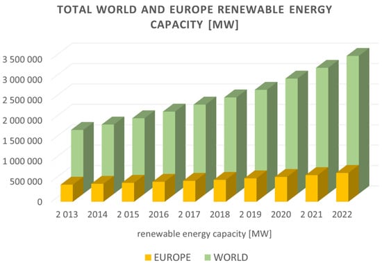
Figure 1.
Total world and European renewable energy capacities in MW (based on data in [3]).
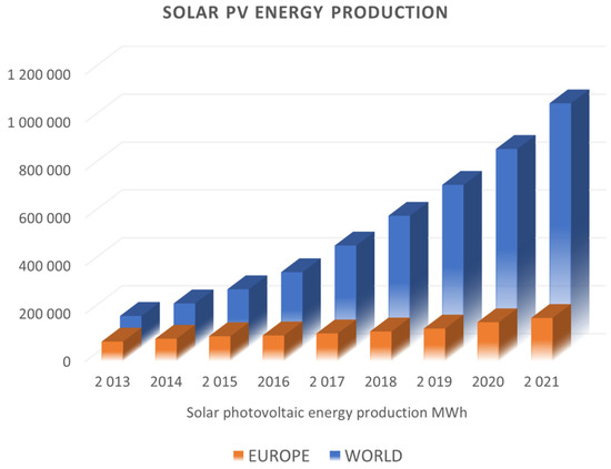
Figure 2.
Solar PV energy production in MWh (based on data in [4]).
As can easily be seen, the development of photovoltaic-based energy systems is quite rapid (Figure 3). Figure 3 shows the growth in the share of installed PV systems compared with other RESs aggregated for the world, Europe, and Poland. The graph illustrates extremely large differences in the changes in the share of PV in the RES mix. In Europe, there is a stable value increasing over 10 years from 19.3% to 31.6%. In the global market, PV shares have increased much faster from a low of 8.8% to 31.2% (authors’ calculations based on [3]). In Poland, on the other hand, the increase is extremely high, ranging from 0.04% in 2013 to 52.5% in 2022. It should be noted here that, when compared with all solar energy sources in general, the global PV share is impressive, reaching over 99% in 2022, though it has been high for a long time and has increased over the last 10 years from 97.7% to 99.1%. The decisive factor for the great popularity of PV systems over photothermal conversion systems, despite the much lower energy conversion efficiency of PV systems, is their direct generation of electricity, which is easy to transmit and convert into other types of usable energy. Furthermore, the popularity of PV systems is strongly influenced by their ease of installation, virtually maintenance-free operation, and relatively low failure rate. They are therefore strongly promoted by individual and subsidised governments [5].
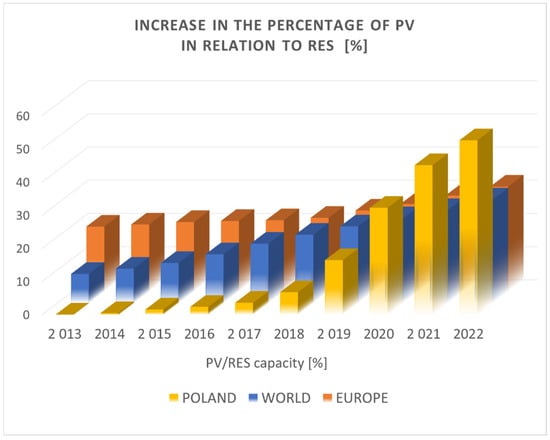
Figure 3.
Percentage PV in total renewable energy capacity as a percentage (based on data in [3]).
In recent years, the capacity of PV systems worldwide has increased from 137.47 GW in 2013 to 1055.03 GW in 2022 (Figure 1). This is an increase of almost eight times. Also, compared with other RESs, PV systems increased their share of the installed capacity from 8.77% in 2013 to 31.19% in 2021 (Figure 2); in other words, PV’s share increased by more than 3.5 times. Accordingly, in these years, the global energy production by PV increased from 131 GWh to 1020 GWh, while the share of PV in RES energy production increased from 2.61% to 12.98%, or an increase of 4.96 times. This leads us to conclude that there is high efficiency and therefore an economic rationale for investing in PV systems. An example of this is Poland, where the share of PV capacity in RESs is as high as 52.57%, and the increase from 2013 to 2022 was more than 1344 times.
The rather strong increase in interest in PV installations observed in recent years has resulted in their incredible development both in terms of technology and the number of PV installations installed annually. Figure 4 shows the potential (installed capacity) of PV systems against the total potential in relation to the installed capacity of RESs for the countries most involved in RES generation. The leading countries in terms of total RES installation capacity in 2022 included Germany, the USA, Canada, France, Spain, Italy, UK, Brazil, Russia, Turkey, China, Japan, India, and Australia. However, not all of them are leaders in terms of installed PV capacity (Figure 4). This fact is generally due to two reasons. The first is geographical location, which limits access to large amounts of solar radiation throughout the year (Canada and Russia). The second is the wealth of these countries, as PV systems are not the cheapest RES. Here, Russia, Brazil, India, and Turkey are examples. It should be noted, however, that these countries obtain a significant part of their RES potential from simple biomass combustion.
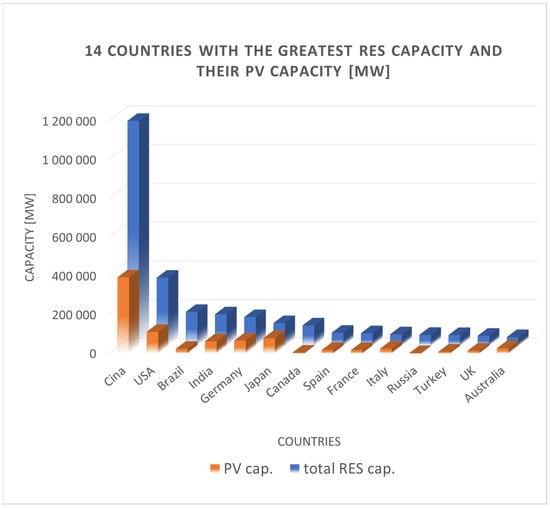
Figure 4.
List of installed RES capacities and installed PV capacities for the 14 leading countries in the RES industry and the percentage share of PV in RESs (based on data in [3]).
Such intensive development of renewable energy sources with weather-forced generation necessitates intensive measures to stabilise the operation of energy distribution and transmission networks. Although operation of the main RES sources (i.e., photovoltaics and wind turbines) is fairly complementary [6], it is becoming necessary to use energy storage. Battery technology (based on rare earth elements), which is currently the market leader, is firstly extremely expensive and secondly not entirely safe. High hopes for energy storage should be pinned on hydrogen technology [7], but along the way, the problems of safe storage and distribution of this gas must be solved. Another idea for energy storage is to use the natural operating conditions of the installations of other renewable energy sources, such as hydroelectric power plants and biogas plants. In [8], the authors draw attention to the large and untapped potential of small hydropower plants (SHPs). In addition to matching energy production to momentary demand, they can perform the retention function necessary for regional hydrological security. In the case of biogas plants, there is a natural energy store in the form of a biogas reservoir. This means that a biogas plant can be used as a peak load power plant, operating at times when generation from wind and photovoltaic sources ceases. The favourable environmental impact of biogas plants results from the replacement of atmospheric emissions of methane from natural rotting processes with carbon dioxide, which has a much lower greenhouse effect. Carbon dioxide is produced by recovering energy from biogas during its combustion. An additional function of a biogas plant can be the use of production waste (digestate) as a natural fertiliser. In [9], it was shown that the digestate from a 1.8 MW biogas plant can be used to fertilise agricultural crops over an area of almost 2000 ha, abandoning the use of artificial fertilisers there entirely or almost entirely. The avoided greenhouse gas emissions from production of the fertiliser required to fertilise this area are equivalent to more than 3000 Mg CO2 per year.
PV systems are currently the fastest growing branch of RESs [10]. This is due to the decreasing costs and increasing efficiency of PV. The increase in efficiency of photovoltaic installations is related to both the continuously improving silicon photovoltaic cell technology and the use of additional design treatments in the manufacture of PV modules. Thus, for example, laser texturing of the inner side of the solar glass [11] results in a better utilisation of incident sunlight on the module’s surface, and the use of appropriate luminophores [12] changes the spectral distribution of light reaching the cell’s surface, increasing the photovoltaic conversion efficiency. However, due to the still quite high cost of PV installations, for their economically viable use, it is necessary to provide PV modules with the best possible operating conditions and, in particular, adequate illumination of them with solar radiation. One of the elements that significantly impair the efficiency of PV panels is their shading, which by reducing the radiant flux reaching the surface reduces their efficiency. It is logical that shade over a large part of a PV module from a chimney, tree, etc. will greatly reduce its efficiency. Attention should also be paid to shading by seemingly small-scale elements such as antenna masts, antennas, lightning protection installations, and overhead power and telecommunication lines, which contrary to appearances can reduce the efficiency of PV systems quite effectively [13]. This paper addresses the problem of researching and modelling the effect of shading from thin, linear overhead elements on the efficiency of PV panels. In addition, the efficiency of PV panels is affected by, among other things, contamination of the panel surface [14] and the temperature which the n-p junction achieves during operation, but these are factors that are beyond our direct control during the installation of PV systems.
Studies on the effect of shading on the operation of PV panels have already been carried out by other researchers. To begin with, a study on uniform shading was conducted for each panel operating in a PV power plant [15]. The authors investigated and carried out simulations in the MATLAB environment for different PV panel connection configurations. The following is the latest research on the impact of shading on PV panels and the suggested methods for reducing it. The basis for this study regarding the effects of shading on PV systems is analysis of the I-V characteristics and, based on them, the detection of shading, as well as the qualitative and quantitative assessment of the phenomenon. Many researchers discussed this topic in their works. For example, the authors of [16] described a method for detecting and categorising shading on photovoltaic (PV) arrays, based on a small amount of measurement data. The developed algorithm relies on detecting the first point of maximum power on the I-V characteristic curve and the value of the equivalent impedance at that point. It can distinguish whether a power drop is caused by reduced illumination across the entire PV array or only partial shading. In the analysis, it was assumed that the solar illumination within the entire single PV module (even when shaded) remained constant. For the algorithm to function correctly, information is required concerning the interconnection structure of modules in the PV array and their catalog electrical parameters. Another paper [17] proposed a new modified tunicate swarm algorithm (MTSA) as a tracker of the maximum power point to increase the level of conversion efficiency of a PV operating in partial shading. The conventional tunicate search algorithm (TSA) is enhanced by incorporating two distinct random numbers to improve the algorithm’s search ability and avoid becoming stuck in local optima. The MTSA controls the duty cycle of the DC-DC converter connected at the terminals of the PV system. Also, in [18], a bionic algorithm for searching for the MPP based on the I-V characteristics of a photovoltaic field was proposed, assuming that some modules included in this field were uniformly shaded over their entire surfaces. The analysis of six shading scenarios showed that the proposed algorithm was able to find the GMPP in less than 0.2 s. The authors of [19] proposed a differential quadrature technique for maximum power point tracking of partial PV array shading. The algorithm using a single-diode, dual-diode, and triple-diode photovoltaic cell model was implemented in the MATLAB Simulink environment. The calculation assumes different irradiation of the individual PV modules forming the chain, with a constant value of irradiation on the surface of a given module. The authors of [20] suggested a controller to determine the maximum power point (MPP) for a PV system operating under various partial shading conditions. Based on the results, it was found that the modified hybrid ANFIS MPPT method based on grey wolf optimisation provided good outcomes. the authors of [21] compared the effectiveness of several MPPT algorithms and whether dynamic shading of a set of photovoltaic cells in a module occurred. It was assumed in the analyses that the irradiance on the surfaces of all photovoltaic cells in the shaded group was the same. The authors of [22] presented an interesting approach to shading, showcasing quantitative analyses of dynamic shading caused by various obstacles such as neighbouring buildings. The reduction in both direct and diffuse radiation due to shading was examined. The authors of [23] described an advanced algorithm for calculating the shadow cast by semitransparent PV modules located on the roof of a greenhouse. In this case, the analysis was also based on creating a binary matrix indicating whether a shadow would appear at a given location on the ground or not. The authors of [24] presented a generalised analytical method for modeling photovoltaic systems under partial shading conditions. The I-V curves were obtained by summing up all the I-V curves for the individual elements of the photovoltaic chain. A two-diode model was used. Bypass and blocking diodes were taken into account as well.
One method for reducing the impact of shading on a system’s PV performance is static [25] and dynamic reconfiguration in a partially shaded PV system [26]. The proposed winnowing method boosts the output power of PV systems while requiring less switching hardware. Other authors [27] proposed improving the efficiency of partially shaded PV panels by using a novel anti-king diagonal sudoku (AKDS) strategy, ensuring the maximum dispersion of shade to attain uniformity in the row current. Another paper [28] proposed a novel meta-heuristic optimisation technique called Vommi to resolve the reconfiguration process of shaded modules in a photovoltaic array. According to the authors, the VOA-based method revealed higher maximum power values. The authors of [29] presented an innovative method for reconfiguring PV arrays in the presence of complex and non-obvious shading shapes. A simulation in a MATLAB Simulink environment was carried out for a PV array of 9 × 9 modules, assuming various shading levels for individual modules. Confirmation of the simulation was realised with a 6 × 6 PV cell array. The authors of [30] offered an adaptive reconfiguration technique for a 4 × 4 PV array. This reconfiguration reduced the complexity and had better shade dispersion. The effectiveness of the proposed reconfiguration technique was implemented in a MATLAB Simulink environment and tested on a 4 × 4 total-cross-tied PV array. The authors of [31] also proposed PV system configuration simulations in the MATLAB Simulink environment. The authors suggest generalised modelling of a photovoltaic (PV) module and different PV array configurations, namely conventional configurations (series, parallel, series-parallel, total-cross-tied, bridge-linked, and honeycomb) and hybrid configurations (series-parallel and total-cross-tied). The authors of [32] presented a method for reconfiguring a shaded PV array called the black widow reconfiguration (BWR). This method was tested for both static and dynamic shading. In contrast, a different approach was presented in [33], where the use of accumulators in the rows of each total-cross-tied (TCT) system was proposed. It eliminates the need for system reconfiguration and the use of bypass diodes. In [34], several algorithms for such a reconfiguration were proposed, which resulted in an increase of up to 16% in the power output of the shaded PV system. The main method of minimising the effect of shading on PV modules is to use bypass diodes. However, due to the cost and technical problems of using multiple bypass diodes in each PV module, they do not perform well for small shadow shapes. As shown in [35], reconfiguration of PV module connections also yields good results with only a simple shadow shape. When there are multiple peaks in the power–voltage characteristics, artificial intelligence, particularly artificial neural networks (ANNs), are used to find the MPP. In the work cited, the following types of ANNs were used: feedforward (FFNN), radial basis function, functional link (FLANN), the adaptive neuro-fuzzy inference system (ANFIS), and a hybrid ANN with classical techniques.
The aforementioned studies were based on the assumption of a constant level of shading on the shaded module at a given moment, which is not an appropriate approach in the case of shading caused by linear structural elements or cables. The authors of [36] offered an in-depth analysis of shading on photovoltaic modules, categorising it as either permanent or temporary. The authors concluded that temporary shading can be alleviated by implementing PV module cleaning and dedusting techniques, while permanent shading can be reduced using PV reconfiguration techniques. The article also includes various techniques for mitigating performance losses from shading.
Researchers are also conducting studies on other parameters of PV panels. For example, the authors of [37] illustrated experimental research on temperature changes in a series-connected chain of PV cells under partial shading conditions. The results indicate that the maximum temperature was reached for shading in the range of 40–60%. The authors of [38] described a thermal-electrical-optical model for photovoltaic blinds installed on a building facade. Dynamic shading effects from various structural elements were taken into account in the model. The authors of [39] also presented an experimental setup creating shading. It consisted of six wooden rotating blinds arranged in two rows: an upper and lower one. The wooden blinds could rotate around horizontal axes, and their height could be adjusted on the mounting structure. To some extent, partial shading is possible because a module placed at an angle provides a weaker cross-section for solar radiation.
A rather comprehensive review of the methods for finding the maximum power point (MPP) in photovoltaic systems is presented in [40]. The authors indicated that in the case of uniform environmental conditions (UECs), the best results are obtained by combining algorithms based on the current–voltage characteristics with algorithms using a mathematical PV array model. On the other hand, for partial shading conditions (PSCs), high hopes can be placed on swarm intelligence optimisation algorithms (SIOAs). However, in the case of SIOAs, the proper selection of three parameters of this algorithm—the startup conditions, dynamic response speed, and cut-off conditions—has an extremely large impact on the final result.
As mentioned above, most researchers dealing with the issue of partial shading in PV systems tend to focus on the macro-analysis of partial shading of photovoltaic modules, which is mainly analysed from the perspective of the impact of shading on the shape of the I-V characteristics of a PV module array. Researchers mainly focus on optimising MPPT algorithms so that in partial shade conditions, they are able to find the global rather than local maximum power of the said characteristics. All of the articles cited assumed that if there were any shading on a PV array, it had a constant value on the surface of a given module. This approach is correct for shadows from large objects. However, shadows coming from objects such as lightning rods or power lines are small and affect only some cells on the module. As shown in [41], in such a case, one cannot assume that the module is uniformly shaded.
An analysis of different types of shading of PV panels by masts, overhead lines, vegetation, bird droppings, other panels, and architectural features was conducted in China [42]. However, the authors limited themselves to analysing the current–voltage I-U characteristics for the different types of shading. The authors also pointed out that partial shading of the module favours the occurrence of hot spots, contributing to a reduced module lifetime and, in extreme cases, module failure. The results of the study show that the shadow area caused by masts and vegetation is not particularly large, but the shadows can spread to several solar cell groups in series for neighbouring modules, which seriously reduces the output of photovoltaic modules. The effect of panel shading by bird droppings on the performance and characteristics of the module is relatively small, as too small a shadow area could not activate the bypass diode due to the applied polarisation voltage in the conduction direction being lower than the diode’s conduction voltage threshold, which nevertheless results in a hot spot. Also, an interesting study on the shading of PV power plant modules by, for example, an overhead power line was carried out in [43]. The authors experimentally analysed through infrared imaging the effect of shading by overhead lines on the formation of hot spots on shaded PV panels. The current–voltage characteristics of shaded and unshaded panels were measured simultaneously. The shaded modules showed negligible hot spots and some reduction in the MPP.
This article represents a significant advancement in comparison with the existing research literature. The authors of the cited analyses and studies focussed on the PV system as a whole, treating individual panels as uniformly shaded photovoltaic sources of electric energy. In this article, on the other hand, shading on the panel surface is meticulously modeled, with a specific focus on its individual cells. Furthermore, the modeling proposed in this work takes into account the umbra, penumbra, and antumbra, enabling calculation of the irradiance on each photovoltaic cell. Therefore, it can be said that the level of detail has increased by an order of magnitude. Based on this model, it is possible to accurately predict the shadow profile at a specific time, date, latitude, and longitude, as well as the location of the shading object and the orientation of the PV surface.
The authors suggest utilising the shading model of individual cells to accurately determine a priori the level of energy production reduction for a given module. Such an analysis is necessary due to the relatively small dimensions of the shadows caused by linear objects in relation to the module’s surface, although not in relation to the surface of a single cell. However, the impact of shading on one cell appears throughout the panel. As demonstrated above, such a detailed approach to shading is not common.
Characteristics of Solar Radiation Reaching the PV Panel Surface
Solar radiation can be divided into three components [44] as shown in Figure 5. These are as follows:
- Direct radiation. This is short-wave radiation with the direction of propagation aligned with the line connecting the Sun and the PV panel surface. The wavelengths of direct solar radiation, which after passing through the atmosphere reach the Earth’s surface at a rate of 98%, range from 0.3 to 2.5 µm. In this range is all visible radiation with wavelengths of 0.4–07 µm, infrared radiation in the IR-a range of 0.7–1.5 µm, and the upper part (1.5–2.5 µm) of infrared radiation in the IR-Bp range, as well as ultraviolet (UV) radiation in the UV-B and UV-A ranges.
- Diffuse radiation. This is the radiation which results from the refraction, reflection, and absorption of direct radiation by the Earth’s atmosphere. This is the cause of the blue radiation in the sky, due to the easier scattering of blue (short-wave) direct radiation from the Sun. Its spectral composition depends on haze, cloud cover, and the purity of the atmosphere. In addition, diffuse radiation includes the long-wave radiation emitted by the atmosphere, which has a much longer wavelength than direct and diffuse solar radiation. It is emitted around the clock in the wavelength range of 4–120 µm. The Liu–Jordan isotropic model for solar radiation reaching the active surface of a photovoltaic panel assumes that diffuse radiation reaches an arbitrarily directed surface uniformly from the entire blue hemisphere.
- Reflected solar radiation (albedo). This is the part of the direct and diffuse radiation reaching the surface of the PV panel which has been reflected by the PV panel’s surroundings in its direction. It depends on the reflectance of the PV panel’s ambient elements and is the product of the sum of the direct and diffuse radiation and the ambient reflectance.

Figure 5.
Solar radiation components in an isotropic model.
Figure 5.
Solar radiation components in an isotropic model.

2. Experiment Confirming the Significant Effect of Small Linear Shading on the Electrical Parameters of a PV Module
2.1. Description and Methodology of the Experiment
Even slight shading of a PV module results in the shaded cells ceasing to act as a generator and becoming a load [45]. The effects of shading in different PV module connection configurations have been presented in studies by many authors. The authors of [46] presented a method for predicting the internal connections of PV modules in a TCT structure. On the other hand, the authors of [47] showed that short PV chains operating separately have the lowest power losses when it comes to operation under partial shading conditions. In [48], optimisation of the connections between PV modules is considered so that the power output is maximised under partial shading conditions. The authors of [49] proposed several PV array arrangements to mitigate the effects of partial shading. The change in I-V characteristics due to partial shading is described by shifting the avalanche breakdown voltage of the shaded PV cells [50]. The authors of [41] presented a two-diode model of PV cells and how to replace the series-parallel arrangement of these cells with a single substitute cell. The authors of [51] described the analysis of serially connected seven-PV modules, which can be replaced by seven cells with suitably selected parameters. The analysis was carried out in the presence of bypass diodes as well as without them. In order to check how the linear shading appearing on the surface of the PV module affects its electrical parameters, a corresponding measurement experiment was carried out. One of the PV installations located within the AGH University of Science and Technology campus in Krakow (GPS: 50°03′58.16″ N, 19°55′17.69″ E) was used for this purpose. The installation under consideration is located on the roof of a building and is partially shaded by a lightning protection system. Using an EKO MP-170 photovoltaic module current–voltage characteristic meter, the electrical parameters of a photovoltaic module made with polycrystalline silicon technology were tested in the absence and presence of linear shading. The module, with dimensions of 1654 × 989 mm, contains 60 series-connected cells 156 × 156 mm in size, which are divided into 3 sections of 20 cells each using bypass diodes. The nominal power of the module is 260 Wp. The vertical lightning conductors have a diameter of 18 mm and a height of 3.5 m above the surface of the modules and are located 36 cm south of their bottom edge. This geometrical arrangement results in a linear shadow moving across the module surface. A view of the installation and the layout of the analysed shading is shown in Figure 6.
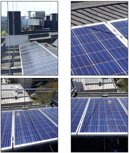
Figure 6.
View of the installation (upper left) and the 3 systems of shading under consideration: Shade No. 1 (upper right), Shade No. 2 (lower left), and Shade No. 3 (lower right).
Prior to the experiment, the module was thoroughly washed, and once the temperature had stabilised, its I-V characteristics were measured, which were then taken as a reference. The entire experiment lasted approximately 3 hours. For each measurement of the I-V characteristics, the irradiance at the surface of the module and its temperature were also measured. During the experiment, the irradiance varied between 799 and 893 W/m2, and the module temperature varied between 44 and 52 °C. For the purpose of this article, four cases of shading were selected for analysis:
- No shade: The shade from the lightning conductor did not reach the module. This measurement was taken as a reference.
- Shade No. 1: The shade covered 3 cells per section.
- Shade No. 2: The shade covered 10 cells per section.
- Shade No. 3: The shade covered 12 cells per section.
Since the I-V characteristics were measured under different irradiance and temperature conditions, they were transposed to STC conditions using the first method described in IEC 60891:2021. The measured characteristics are shown in Figure 7, and the most important electrical parameters are shown in Table 1.
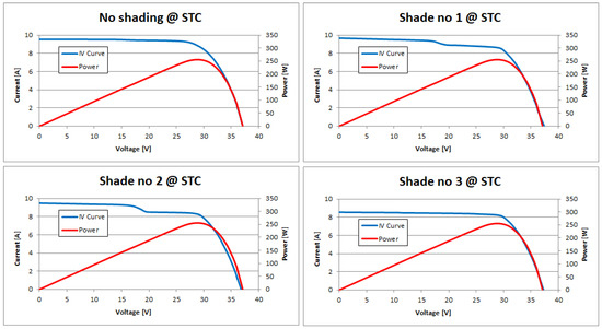
Figure 7.
I-V characteristics for different cases of shading.

Table 1.
Electrical performance of the module under different shading variants.
2.2. Conclusions from the Experiment
Even a seemingly small linear shading covering three cells (two significantly and one minimally) reduced the power generated by the module by 1.4%. A shadow covering more cells could reduce the power by more than 6%. It is important, however, to carefully analyse the geometry of this shade and its interaction with the individual cells in the module because, as the cases of Shade No. 2 and Shade No. 3 show, it was not only the number of cells covered by the shade that affected the power generated by the module but also their distribution in relation to the section as well as the degree of shading of these cells. The operation of the bypass diodes in the PV module was puzzling. In the case of Shade No. 1 and Shade No. 2, the layout of the shade on the module suggested the activation of only one bypass diode. This is reflected in the shape of the recorded current–voltage characteristics. However, in the case of Shade No. 3, the shadow layout suggests the activation of two bypass diodes, while the current–voltage characteristics show that all three bypass diodes in the module were activated. This phenomenon requires further research in the future through a series of measurement experiments and simulation work in the MATLAB Simulik environment. Thanks to the mathematical model of shading proposed in this article, it is possible to accurately simulate irradiance values individually on each photovoltaic cell included in the module. These issues will be the subject of the authors’ next article.
3. Shade Modelling
3.1. Methodology
Sunlight does not fall from a single direction of the celestial sphere but from a certain area of it (solid angle). This area is referred to as the solar disk and is the visible image of the luminous sphere that is the Sun as a star, specifically its photosphere. The solar disk on the celestial sphere is a circle whose angular diameter varies between 31′31″ and 32′33″ as a result of the varying distance between the Earth and the Sun, due to the ellipticity of the Earth’s orbit. In these considerations, we focussed on direct radiation (i.e., from the solar disc), as the degree of its obscuration would determine the degree of shading of a given area of a photovoltaic surface. Since the analysed objects casting shade were quite close on a cosmic scale, it was safe to assume that they did not reduce scattered or reflected light. (An example of shading which does not meet this assumption is an eclipse of the Sun by the Moon, since not only is direct radiation reduced but also diffuse and therefore reflected radiation.) In these considerations, we treated the diffuse and reflected radiation as constant values, independent of the degree of shading of the solar disc. Therefore, the value of diffuse and reflected radiation had to be subtracted from the total radiation, and we treated the shaded area as an area with zero radiation value and the completely unshaded area as an area with full brightness which, for the purposes of analysing and modelling shading, we treated as an illumination value with a dimensionless unit value. In order to make such a model consistent with reality, the light component associated with the reflected and diffuse light radiation had to ultimately be added to the areas illuminated by the sun disc which were completely, partially, or fully shaded.
As already mentioned, the Sun in the sky is a disc and not a point, and its light may reach a selected point on a surveyed surface from the whole surface of the solar disc or from part of it, or it may not reach at all. If sunlight reaches the selected point from the whole disc, then the point is fully illuminated, and the area is referred to as full light. If light only reaches a point from part of the solar disc, then the point belongs to the penumbra (semi-shadow) area. Places that are not illuminated at all by the Sun’s disc belong to the umbra (shadow). The area which receives light from opposite parts of the Sun’s disc, while the central part of the disc which is obscured is called the antumbra. If the Sun were a point of light, then there would be no penumbra or antumbra area at all. In the present discussion, we assume that the objects providing the shading are long, straight objects with circular cross-sections. These objects represent antennas, power lines, and other long and narrow structural elements which occasionally cast shading on the surfaces of photovoltaic modules.
A diagram of the formation of the umbra, penumbra, and antumbra is shown in Figure 8. In Figure 8, the solar disc is not marked as, geometrically, it is infinitely far away, and the light rays coming from its specific points are parallel. However, the directions of the Sun’s rays defining the boundaries of the individual shading elements are marked. This figure shows a circular cross-section of a linear object creating shade.
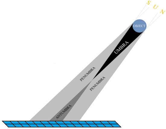
Figure 8.
Diagram of the umbra, penumbra, and antumbra from a circular object, where the projection screen is the PV module.
The geometrical conditions for the formation of the umbra, penumbra, and antumbra impose the way in which they are modelled. When the distance between the object and the screen (in this discussion, the PV surface) is zero, only the umbra is present. When this distance increases, however, the umbra narrows, and the penumbra expands, as shown in Figure 8. At a sufficient distance, the umbra disappears, and only the penumbra remains. When the distance between the object and the surface continues to increase, the penumbra continues to expand, and the umbra is replaced by an antumbra, which also increases in size. The intensity of sunlight decreases steadily along the profile of the penumbra in a continuous manner from the area of full brightness to the penumbra-umbra boundary or the penumbra-antumbra boundary. The umbra area will have a constant brightness of zero, while in the antumbra area, the brightness changes in such a way that it is smallest at its centre.
3.2. Mathematical Description of the Shading Phenomenon Originating from Sunlight
For the case of a perpendicular cross-section in the penumbra area at such a distance that the umbra is also present, a diagram of the geometrical arrangement for the formation of shade is shown in Figure 9.
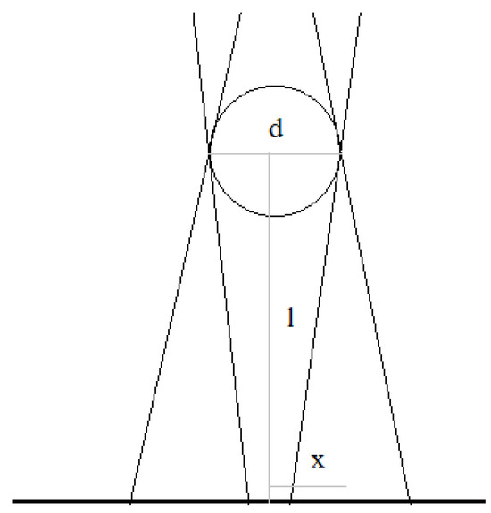
Figure 9.
Diagram of the umbra and penumbra cast perpendicularly on the surface with the marked quantities d (rod diameter), l (distance of the object from the surface), and x (lateral distance from the shade axis).
Geometrical analysis of this case leads to the derivation of a mathematical formula for the brightness profile of the penumbra. This profile as well as the antumbra profile (for larger distances l) can be expressed by Equations (1) and (3). Figure 10 shows the brightness profiles for an object with a diameter d = 0.15 (in meters) and for different distances l.
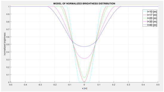
Figure 10.
Examples of shading profiles for object diameter d = 0.15 (m) and selected distances l between the object and the projection screen.
The analytical formula describing the brightness profile L(x,l,d) of the penumbra for the case where the umbra is in the centre of the shaded area is described by Equation (1):
where
In the case of the antumbra, the brightness profile L(x,l,d) is expressed by Equation (3):
where
and
Examples of brightness profiles are shown in Figure 10.
In order to model the shading distribution on the PV module occurring due to the presence of a linear object (rod) obscuring the module, the spatial orientations of the Sun, the PV module, and the linear object need to be determined. Each of these orientations can be described by two angles: the azimuth and angular height. The azimuth of the Sun is defined as the angle in the horizontal plane calculated from the southern direction to the centre of the solar disk to the east (negative) and to the west (positive). The altitude for the Sun is defined as the angle in the vertical plane between the horizontal line and the direction pointing to the centre of the solar disc, which is positive when the Sun is above the horizontal line and negative when it is below it. The azimuth and altitude of the rod are also defined as the respective angles with respect to the horizontal plane. Finally, the azimuth and elevation of the PV module plane are defined as follows. The azimuth determines the angle by which the PV module should be rotated about the vertical axis (Figure 11), assuming that the PV module is initially oriented horizontally, with its longer sides pointing in the north-south direction. The altitude, in turn, determines at what angle (after a previous horizontal rotation) the PV module should be tilted around an axis in the PV plane and connected to the centres of the PV module’s longer sides (Figure 12).
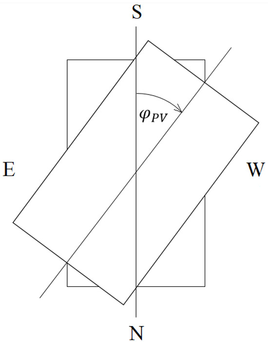
Figure 11.
Rotation of the PV plane at an angle in the horizontal plane.
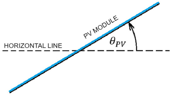
Figure 12.
Slope of the PV plane at an angle in the vertical direction.
The mathematical formula for the matrix of rotation of the coordinate system about any vector and at any angle should be used [52]. This matrix is expressed in Equation (6):
In the above notation, rotation at an angle θ occurs around the vector .
This matrix can be used to realise a compound of two rotations. The first rotation is around the vector z = [0 0 1]T at an angle equal to the azimuth PV (i.e., ), while the second rotation is around the vector x = [1 0 0]T at an angle equal to the PV height (i.e., ). These matrices are of the form in Equations (7) and (8):
The azimuth and elevation relative to the PV plane can be calculated as shown in Equation (9):
where v is the position vector of the Sun in the horizontal system. Using the spherical system, the vector v can be expressed by the azimuth , height , and the distance to the Sun R using Equation (10):
Similarly, the resultant vector w can be represented as shown in Equation (11) with the new angles of the azimuth of the Sun relative to the PV and elevation of the Sun relative to the PV , with this being the PV plane that will be arbitrarily oriented with respect to the horizon, as well as the distance to the Sun R. Of course, the distance to the Sun R in the geometric sense is infinitely large, but it disappears in the final mathematical formulas:
From the vector w, and can be calculated according to Equations (12) and (13):
Detailed analyses of these calculations are provided in the m-file source code (for the MATLAB environment) with appropriate comments.
In a similar way, the azimuth and elevation of the rod with respect to the horizon can be converted to the azimuth and elevation of the rod with respect to the PV plane.
Based on mathematical considerations, the shade length of the rod g can be calculated:
where
Here, l is the rod length, is the angle formed by the plane defined by the rod and its shadow with the PV plane, is the azimuth of the rod in relation to the PV plane, is the rod height in relation to the PV plane, is the azimuth of the Sun in relation to the PV plane, is the Sun’s altitude in relation to the PV plane, is the azimuth of the rod’s shadow in relation to the PV plane, and th is the thickness of the rod’s shadow divided by the thickness of the rod.
This article is accompanied by three m-files (MATLAB files) in which the shading model and coordinate system transformations were performed. In the shadow.m file, a function is realised which calculates the degree of shading depending on the value of the deviation from the shadow axis, the distance from the object casting the shadow, and its diameter (Figure 9). The transformation.m file then shows the transition from the horizontal layout to the layout associated with the plane of the PV module. The file shadow_calculation.m allows the calculation of the parameters of the shadow, the Sun, and the rod (the object casting the shadow in the layout related to the PV plane). Each of the above files contains extensive comments explaining the calculations with references to the relevant sections of this article.
4. Experimental Verification of the Shade Modelling Results on a PV Module
Measurements were made of the shade coming from a cylinder positioned vertically on a horizontal plane. A diagram of the location of the cylinder casting the shade is shown in Figure 13, and an actual view of the experimental stand is shown in Figure 14. Illumination measurements were made with a precision light meter sensor recording the light intensity, fitted with a 4 mm-wide linear aperture. The illumination profile was measured in a line perpendicular to the shadow line. The position of the sensor was determined using a digital ruler with a resolution of 0.01 mm. The results in the form of measurement points marked with blue asterisks are shown in Figure 15. The red line in this figure indicates the shading profile according to the model, while the green graph is a filtered red graph using a sliding window of 4 mm, which corresponds to the illumination recorded by the sensor. Thus, it is reasonable to compare the measured data with the red graph as well as the green graph, as can be seen in Figure 15.
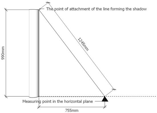
Figure 13.
Shading cylinder location diagram.

Figure 14.
View of the test bench during the experiment.
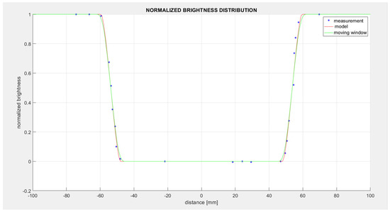
Figure 15.
Normalised brightness distribution according to measurements, model, and model after filtering with a sliding window.
The measured data from the experiment are shown in Table 2.
Table 2.
Measurement data.
For the purposes of mathematical modelling, the shadow was assumed to have a brightness of zero, and the full illumination had a brightness of unity. Scaling equations (Equations (23) and (24)) were used:
where 84.5 (mm) is the measured shadow centre, 13 (W/m2) is the measured value of the light flux, taken as the value corresponding to the shadow (diffuse and reflected radiation alone), 181 (W/m2) is the maximum measured value of luminous flux, considered as no shading (full light).
Normalised distance = Distance − 84.5
Normalised brightness = (Brightness − 13)/181
Although the minimum irradiance obtained from the measured data was 12 W/m2, the value of 13 W/m2 was considered to be more reliable as a minimum value, and it was taken to mean full shade (umbra).
Figure 16 and Figure 17 graphically show the residuals and differences between the measured data and both the brightness profile model (original model) and the modified brightness profile model (moving window model). Figure 16 shows the residuals and differences for the normalised raw measurement results in relation to the results obtained by applying the developed model.
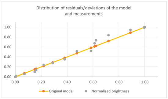
Figure 16.
Distribution of residuals and deviations for the original model and measurements.
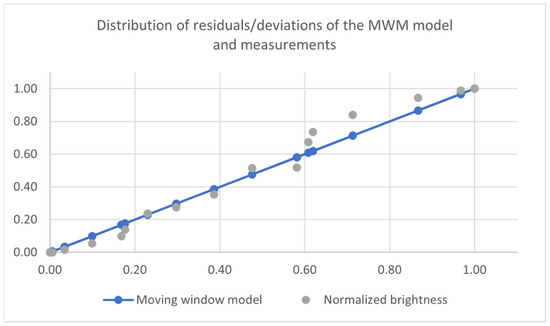
Figure 17.
Distribution of residuals and deviations for the original model + MWM.
The graph in Figure 17, on the other hand, shows the residuals and deviations for the normalised raw measurement results in relation to the results obtained from the model developed and then processed by the moving window model. The aim was to obtain data more similar to the measurements taken with a 4 mm-wide slit (window).
As the graphical comparison of the two relationships did not give clear results regarding the quality of each model, a statistical verification was carried out to test their quality, determining the degree of fit to the measurement data obtained with the results calculated in the model and those processed by the moving window model’s formula. The analysis was performed for normalised data. The following parameters were calculated:
- Pearson’s linear correlation coefficient r tells us about the strength and direction of the relationship between variables. A coefficient value of one indicates a perfect linear relationship.
- The determination coefficient R2 measures the proportion of variation in the explanatory variable, which is explained by the linear effect of the explanatory variable.
- The convergence coefficient Ⴔ, which complements R2, indicates which part of the measurement results is not explained by the model.
- The fitting coefficient d refers to the ratio of the maximum residual or deviation to its mean value.
The results obtained are shown in Table 3.
Table 3.
Results of the analysis of the model’s fit to the measurement data.
In the case under consideration, due to standardisation, the relative error could not be calculated, as the values occurring in the denominator took on a value of zero, making the calculation impossible.
The results show that the model represented the measured data quite well (r = 0.09943, R2 = 0.9886). When the data were processed in the moving window model (MWM), the fit parameters decreased slightly (r = 0.994303, R2 = 0.988638). However, the fitting coefficient d, which is sensitive to the maximum deviation of the results and the model, increased, which was due to the “smoothing of the original model” by the MWM operation. On the basis of the results obtained, it can be concluded that it was quite well developed, and it was likely that the minimum discrepancies created were much more influenced by measurement errors than by the model not fitting.
5. Uncertainty and Measurement Error
Measurement uncertainty is a parameter associated with a measurement result, characterising the dispersion of values that can be reasonably attributed to the measured quantity (“uncertainty” is always a number).
Measurement uncertainty depends on many potential sources of influence, including the following:
- Incomplete definition of the measured quantity;
- Imperfections in the technical characteristics of the instrument (hysteresis, spread of indications, or specified resolution);
- Imperfect realisation of the measured quantity;
- Non-representative measurements, the results of which may not represent the measured quantity;
- Incomplete knowledge of the influence of external conditions on the measurement procedure;
- Subjective observer errors in reading analog instrument indications (parallax error);
- Limited resolution or threshold sensitivity of the instrument;
- Inaccurately known values assigned to standards and reference materials;
- Inaccurately known values of constants and other parameters obtained from external sources and used in data processing procedures;
- Simplifying approximations and assumptions used in measurement methods and procedures.
This section focuses on the analysis of measurement errors resulting from the accuracy of measuring devices. The limiting error values, the minimum error, and the maximum error for the measured quantities analysed in this article are expressed by the formula
where δ is the instrument class, R is the instrument’s measurement range, and x is the measured value.
Below is an analysis of the measurement errors for the experimental verification of the PV panel shading model.
The absolute maximum errors of the light intensity measurements (E) were found for an instrument class δ of ±2.5, instrument measurement range R of 1999 W/m2, z, correction factor resulting from the use of a linear aperture z, and measured light intensity x of Emin = 12 W/m2 and Emax = 194 W/m2. The errors were as follows. The minimum error was ±10.12 W/m2, and the maximum error was ±15.13 W/m2.
The absolute maximum errors of the sensor position measurements x were found for an instrument class δ of ±0.05, instrument measurement range R of 600 mm, and measured sensor position x of xmin = ±34.03 mm and xmax = ±154.21 mm. The errors were as follows. The minimum error was ±0.1319 mm, and the maximum error was ±0.2970 mm.
The absolute maximum errors of the current–voltage characteristics, temperature, and irradiation measurements for the experiment from Section 2 follow. The absolute voltage measurement error U was found for an instrument class δ of ±1.0, instrument measurement range R of 100 V, and measured voltage x of Umin = 0.00 V and Umax = 37.43 V. The errors were as follows. The minimum error was ±1.000 V, and the maximum error was ±1.378 V.
The absolute current measurement error I was found for an instrument class δ of ±1.0, instrument measurement range R of 10.0 A, and measured current x of Imin 0.00 A and Imax 9.66 A. The errors were as follows. The minimum error was ±0.1000 A, and the maximum error was ±0.2626 A.
The absolute temperature measurement error T was found for an instrument class δ of ±1.5, instrument measurement range R of 100 °C, and measured PV module temperature x of Tmin = 44 °C and Tmax = 52 °C. The errors were as follows. The minimum error was ±1.444 °C, and the maximum error was ±1.525 °C.
The absolute irradiation measurement error Ee was found for an instrument class of δ ±1.5, instrument measurement range R of 1500 W/m2, and measured irradiation x of Eemin = 799 W/m2 and Eemax = 893 W/m2. The errors were as follows. The minimum error was ±34.53 W/m2, and the maximum error was ±35.95 W/m2.
6. Summary
This article presents the problem of partial shading of PV panels by long and thin objects, such as power lines. As a result of the falling shadow and penumbra from a particular linear object, individual PV cells receive weaker irradiance compared with those that are completely unshaded. This results in a decrease in the amount of electricity generated. Due to the design of PV panels, this is much greater than can be accounted for by a reduction in the overall or summary irradiance per PV panel. With such a simple measurement experiment, it was shown that even a shadow from a thin lightning rod can reduce the power output of a PV module by approximately 6%. A mathematical model of the umbra, penumbra, and antumbra shadow brightness profile was developed. For the developed model, source code was prepared for calculations in the MATLAB environment, simulating the appearance of the umbra, penumbra, and antumbra at any orientation and distance from the object casting shade on the PV panel’s surface. The orientation of the PV panel itself and the position of the Sun in the sky in this model can also be arbitrary. An experiment verifying the developed mathematical model was presented, together with statistical treatment of its results. When comparing the experiment with the model, the diffuse component of the illumination was filtered out, focusing on the direct illumination coming from the solar disc. Due to the high location of the test site and the lack of high albedo elements, the reflected radiation component was assumed to be zero. Since the measuring device collected (measured) light from a certain photosensitive surface, a modification of the shading model was introduced by filtering the brightness profile of the original model through a sliding window with the width of the light-collecting area of the measuring device used. Such a modified model was also compared with experimental data, as was the original model. The results of the comparison indicate that the mathematical model adopted, both original and modified, proved to be valid.
7. Conclusions
The umbra, penumbra, and antumbra brightness profile models proposed in this paper reflect the actual distribution of direct radiation intensity on a PV module’s surface shaded by linear structural elements quite well.
The original model explained the measurement data to an exceptionally high degree, obtaining a quite high R2 determination coefficient of over 0.9986.
The moving window model, by “smoothing” the results, achieved a higher degree of fit (d = 0.992360) which was sensitive to the maximum deviations, in spite of a lower degree of explanation of the measurements (compatibility of the measurements with the model), where R2 = 0.9867.
For the measurement devices used, the absolute error increased with the measured value. However, due to the wide range of measured data, the relative errors were quite large for small measured values.
In order to model the actual shading distribution for the linear elements on the surface of the PV module, it is necessary to use accurate data on the intensity of solar radiation (direct, diffuse, and reflected), the position of the Sun in the sky, as well as the orientation of the PV module and the position and orientation of the shading element.
Measurements of the irradiance distribution on the shaded PV module should be carried out over as short a period of time as possible so that the Sun does not change its position relative to the PV module surface and the irradiance conditions do not change due to meteorological conditions.
The drop in PV module efficiency during shading with thin linear objects is much greater than would be implied by the ratio of irradiance and the area of the shaded and unshaded parts of the PV panel (i.e., the PV module’s efficiency is not proportional to the inverse of its shading (the size of the module illumination)).
The mathematical model proposed in this article allows precise calculation of the shadows (taking into account the umbra, penumbra, and antumbra) created by thin linear objects on an arbitrary oriented plane. By replacing the plane with a photovoltaic module having an arbitrary array of photovoltaic cells (understood as rectangles or squares), it becomes possible to calculate the shadow and, consequently, the irradiance separately on each photovoltaic cell. When knowing the location and geometry of the PV installation, it is possible to predict the shadow and its effect on the current–voltage characteristics before a shadow occurs. This will allow, for example, automatic reconfiguration of the connection of photovoltaic modules before they stop working under MPP conditions, as is the case with current algorithms. This is a quite significant novelty of our research compared with other studies reported thus far in leading energy journals. Such a precise analysis is necessary due to the relatively small dimensions of shadows caused by linear objects in relation to the module’s surface but not in relation to the surface area of a single cell.
The qualitative and quantitative assessment of the phenomenon of shading by linear structural elements and cable networks is the subject of further research by the authors. These are based on accurate measurements of the current–voltage characteristics of PV modules as a function of different types of shading. In addition, the authors are developing a model for the energy balance of a PV cell as a function of partial shading, which will be presented in the next article.
Author Contributions
Conceptualisation, J.T., W.K. and M.J.; methodology, J.T., W.K. and M.J.; software, W.K.; validation, M.J.; formal analysis, J.T. and M.J.; investigation, J.T., W.K. and M.J.; resources, J.T. and W.K.; data curation, M.J.; writing—original draft preparation, J.T., W.K. and M.J.; writing—review and editing, J.T., W.K. and M.J.; visualisation, J.T., W.K. and M.J.; supervision, J.T. All authors have read and agreed to the published version of the manuscript.
Funding
This research received no external funding.
Data Availability Statement
Measurement data and MATLAB files are available upon request from the corresponding author. The data are not publicly available because the authors of the article want to have full knowledge of the use of their research results.
Conflicts of Interest
The authors declare that they have no known competing financial interests or personal relationships that could have appeared to influence the work reported in this paper.
References
- Sekhar, V.R.; Pradeep, P. A Review Paper on Advancements in Solar PV Technology, Environmental Impact of PV Cell Manufacturing. Int. J. Adv. Res. Sci. Commun. Technol. (IJARSCT) 2021, 8, 485–492. [Google Scholar] [CrossRef]
- Udayakumar, M.D.; Anushree, G.; Sathyaraj, J.; Manjunathan, A. The impact of advanced technological developments on solar PV value chain. Mater. Today Proc. 2021, 45, 2053–2058. [Google Scholar] [CrossRef]
- Renewable Capacity Statistics 2023; International Renewable Energy Agency (IRENA): Abu Dhabi, United Arab Emirates, 2023; ISBN 978-92-9260-525-4.
- Renewable Energy Statistics 2023; International Renewable Energy Agency (IRENA): Abu Dhabi, United Arab Emirates, 2023; ISBN 978-92-9260-537-7.
- Ding, H.; Zhou, D.Q.; Liu, G.Q.; Zhou, P. Cost reduction or electricity penetration: Government R&D-induced PV development and future policy schemes. Renew. Sustain. Energy Rev. 2020, 124, 109752. [Google Scholar] [CrossRef]
- Hassan, Q.; Algburi, S.; Sameen, A.Z.; Salman, H.M.; Jaszczur, M. A review of hybrid renewable energy systems: Solar and wind-powered solutions: Challenges, opportunities, and policy implications. Results Eng. 2023, 20, 101621. [Google Scholar] [CrossRef]
- Hassan, Q.; Algburi, S.; Sameen, A.Z.; Zuhair, A.; Jaszczur, M.; Salman, H. Hydrogen as an energy carrier: Properties, storage methods, challenges, and future implications. Environ. Syst. Decis. 2024, 44, 327–350. [Google Scholar] [CrossRef]
- Kałuża, T.; Hämmerling, M.; Zawadzki, P.; Czekała, W.; Kasperek, R.; Sojka, M.; Mokwa, M.; Ptak, M.; Szkudlarek, A.; Czechlowski, M.; et al. The hydropower sector in Poland: Barriers and the outlook for the future. Renew. Sustain. Energy Rev. 2022, 163, 112500. [Google Scholar] [CrossRef]
- Kowalczyk-Juśko, A.; Pochwatka, P.; Mazurkiewicz, J.; Pulka, J.; Kępowicz, B.; Janczak, D.; Dach, J. Reduction of Greenhouse Gas Emissions by Replacing Fertilizers with Digestate. J. Ecol. Eng. 2023, 24, 312–319. [Google Scholar] [CrossRef]
- Eze, V.H.U.; Ernrst, E.; Kalyankolo, U.; Okafor, O.W.; Ugwu, C.; Ogenyi, F.C. Overview of Renewable Energy Power Generation and Conversion (2015–2023). Eurasian J. Sci. Eng. 2023, 4, 105–113. [Google Scholar]
- Drabczyk, K.; Sobik, P.; Kulesza-Matlak, G.; Jeremiasz, O. Laser-Induced Backward Transfer of Light Reflecting Zinc Patterns on Glass for High Performance Photovoltaic Modules. Materials 2023, 16, 7538. [Google Scholar] [CrossRef]
- Sibiński, M. Review of Luminescence-Based Light Spectrum Modifications Methods and Materials for Photovoltaics Applications. Materials 2023, 16, 3112. [Google Scholar] [CrossRef]
- Abdelaziz, G.; Hichem, H.; Chiheb, B.R.; Rached, G. Shading effect on the performance of a photovoltaic panel. In Proceedings of the 2nd IEEE International Conference on Signal, Control and Communication (SCC) 2021, Tunis, Tunisia, 20–22 December 2021. [Google Scholar] [CrossRef]
- Teneta, J.; Janowski, M.; Bender, K. Analysis of the Deposition of Pollutants on the Surface of Photovoltaic Modules. Energies 2023, 16, 7749. [Google Scholar] [CrossRef]
- Ramaprabha, R.; Mathur, B.L. A Comprehensive Review and Analysis of Solar Photovoltaic, Array Configurations under Partial Shaded Conditions. Int. J. Photoenergy 2012, 2012, 120214. [Google Scholar] [CrossRef]
- Gupta, A.K.; Singh, R.; Kumar, S. I–V Characteristics-Based Shading Detection Technique for PV Applications. Trans. Indian Natl. Acad. Eng. 2023, 8, 607–615. [Google Scholar] [CrossRef]
- Fathy, A.; Ame, D.A.; Al-Dhaifallah, M. Modified tunicate swarm algorithm-based methodology for enhancing the operation of partially shaded photovoltaic system. Alex. Eng. J. 2023, 79, 449–470. [Google Scholar] [CrossRef]
- Fu, C.; Zhang, L. A novel method based on tuna swarm algorithm under complex partial shading conditions in PV system. Sol. Energy 2022, 248, 2840. [Google Scholar] [CrossRef]
- Ragb, O.; Bakr, H. A new technique for estimation of photovoltaic system and tracking power peaks of PV array under partial shading. Energy 2023, 268, 126680. [Google Scholar] [CrossRef]
- Hussaian Basha, C.; Palati, M.; Dhanamjayulu, C.; Muyeen, S.M.; Prashanth, V. A novel on design and implementation of hybrid MPPT controllers for solar PV systems under various partial shading conditions. Sci. Rep. 2024, 14, 1609. [Google Scholar] [CrossRef] [PubMed]
- Shaikh, A.M.; Shaikh, M.F.; Shaikh, S.A.; Krichen, M.; Rahimoon, R.A.; Qadir, A. Comparative analysis of different MPPT techniques using boost converter for photovoltaic systems under dynamic shading conditions. Sustain. Energy Technol. Assess. 2023, 57, 103259. [Google Scholar] [CrossRef]
- Xu, L.; Ding, P.; Zhang, Y.; Huang, Y.; Li, J.; Ma, R. Sensitivity analysis of the shading effects from obstructions at different positions on solar photovoltaic panels. Energy 2024, 290, 130229. [Google Scholar] [CrossRef]
- Petrakis, T.; Thomopoulos, V.; Kavga, A.; Argiriou, A.A. An algorithm for calculating the shade created by greenhouse integrated photovoltaics. Energ. Ecol. Environ. 2023, 9, 272–300. [Google Scholar] [CrossRef]
- Kermadi, M.; Chin, V.J.; Mekhilef, S.; Salam, Z. A fast and accurate generalized analytical approach for PV arrays modeling under partial shading conditions. Sol. Energy 2020, 208, 753–765. [Google Scholar] [CrossRef]
- Sakthivel, G.; Winston, D.P.; Kumar, B.P.; Ilhami, C. Power enhancement in PV arrays under partial shaded conditions with different array configuration. Heliyon 2024, 10, e23992. [Google Scholar] [CrossRef]
- Kumar, S.K.; Winston, D.P. Performance analysis of winnowing dynamic reconfiguration in partially shaded solar photovoltaic system. Sol. Energy 2024, 268, 112309. [Google Scholar] [CrossRef]
- Ramachandra, N.; Natarajan, R. An efficient power extraction approach for roof-top photovoltaic systems under immobile shade scenarios. J. Clean. Prod. 2023, 429, 139312. [Google Scholar] [CrossRef]
- Kumar, P.R.; Kumar, M.; Babu, T.S.; Kumar, S.N.; Kuchhal, P.; Minai, A.F.; Sharma, A. Study on Meta-heuristics techniques for shade dispersion to enhance GMPP of PV array systems under PSCs. Sustain. Energy Technol. Assess. 2023, 58, 103353. [Google Scholar] [CrossRef]
- Ahluwalia, D.; Anjum, S.; Mukherjee, V. Boost in energy generation using robust reconfiguration: A novel scheme for photovoltaic array under realistic fractional partial shadings. Energy Convers. Manag. 2023, 290, 117211. [Google Scholar] [CrossRef]
- Murugesan, P.; Winston, D.P.; Murugesan, P.; Solaisamy, N.K. One-step adaptive reconfiguration technique for partial shaded photovoltaic array. Sol. Energy 2023, 26, 111949. [Google Scholar] [CrossRef]
- Jha, V. Generalized modelling of PV module and different PV array configurations under partial shading condition. Sustain. Energy Technol. Assess. 2023, 56, 103021. [Google Scholar] [CrossRef]
- Satpathy, P.R.; Aljafari, B.; Thanikanti, S.B.; Sharma, R. An efficient power extraction technique for improved performance and reliability of solar PV arrays during partial shading. Energy 2023, 282, 128992. [Google Scholar] [CrossRef]
- Murugesan, P.; Winston, D.P.; Murugesan, P.; Periyasamy, P. Battery based mismatch reduction technique for partial shaded solar PV system. Energy 2023, 272, 127063. [Google Scholar] [CrossRef]
- Pillai, D.S.; Prasanth Ram, J.P.; Shabunko, V.; Kim, Y.-J. A new shade dispersion technique compatible for symmetrical and unsymmetrical photovoltaic (PV) arrays. Energy 2021, 225, 120241. [Google Scholar] [CrossRef]
- Olabi, A.G.; Abdelkareem, M.A.; Semeraro, C.; Radi, M.A.; Rezk, H.; Muhaisen, O.; Al-Isawi, O.A.; Sayed, E.T. Artificial neural networks applications in partially shaded PV systems. Therm. Sci. Eng. Prog. 2023, 37, 101612. [Google Scholar] [CrossRef]
- Mathew, D.; Ram, J.P.; Kim, Y.-J. Unveiling the distorted irradiation effect (Shade) in photovoltaic (PV) power conversion—A critical review on Causes, Types, and its minimization methods. Sol. Energy 2023, 266, 112141. [Google Scholar] [CrossRef]
- Hong, Y.; Zhu, M.; Sun, K.; Gao, J.; Shan, C. Research on temperature anomalies caused by the shading of individual solar cells in photovoltaic modules. Sol. Energy 2024, 269, 112343. [Google Scholar] [CrossRef]
- Luo, Y.; Zhang, L.; Su, X.; Liu, Z.; Lian, J.; Luo, Y. Improved thermal-electrical-optical model and performance assessment of a PV-blind embedded glazing façade system with complex shading effects. Appl. Energy 2019, 255, 113896. [Google Scholar] [CrossRef]
- Piccoli, E.; Dama, A.; Dolara, A.; Leva, S. Experimental validation of a model for PV systems under partial shading for building integrated applications. Sol. Energy 2019, 183, 356–370. [Google Scholar] [CrossRef]
- Li, J.; Wu, Y.; Ma, S.; Chen, M.; Zhang, B.; Jiang, B. Analysis of photovoltaic array maximum power point tracking under uniform environment and partial shading condition: A review. Energy Rep. 2022, 8, 13235–13252. [Google Scholar] [CrossRef]
- Ishaque, K.; Salam, Z.; Syafaruddin. A comprehensive MATLAB Simulink PV system simulator with partial shading capability based on two-diode model. Solar Energy 2011, 85, 2217–2227. [Google Scholar] [CrossRef]
- Sun, Y.; Chen, S.; Xie, L.; Hong, R.; Shen, H. Investigating the Impact of Shading Effect on the Characteristics of a Large-Scale Grid-Connected PV Power Plant in Northwest China. Int. J. Photoenergy 2014, 2014, 763106. [Google Scholar] [CrossRef][Green Version]
- Dolara, A.; Lazaroiu, G.C.; Ogliari, E. Efficiency analysis of PV power plants shaded by MV overhead lines. Int. J. Energy Environ. Eng. 2016, 7, 115–123. [Google Scholar] [CrossRef]
- Duffie, J.A.; Beckman, W.A. Solar Engineering of Thermal Processes; John Wiley & Sons, Inc.: Hoboken, NJ, USA, 2013; ISBN 978-0-470-87366-3. [Google Scholar]
- Kreft, W.; Filipowicz, M.; Żołądek, M. Reduction of electrical power loss in a photovoltaic chain in conditions of partial shading. Opt.-Int. J. Light Electron Opt. 2019, 202, 163559. [Google Scholar] [CrossRef]
- Pareek, S.; Dahiya, R. Enhanced power generation of partial shaded photovoltaic fields by forecasting the interconnection of modules. Energy 2016, 95, 561–572. [Google Scholar] [CrossRef]
- Mäki, A.; Valkealahti, S. Power Losses in Long String and Parallel-Connected Short Strings of Series-Connected Silicon-Based Photovoltaic Modules Due to Partial Shading Conditions. IEEE Trans. Energy Convers. 2012, 27, 173–183. [Google Scholar] [CrossRef]
- Villa, L.F.L.; Picault, D.; Raison, B.; Bacha, S.; Labonne, A. Maximizing the Power Output of Partially Shaded Photovoltaic Plants Through Optimization of the Interconnections Among Its Modules. IEEE J. Photovolt. 2012, 2, 154–163. [Google Scholar] [CrossRef]
- Belhaouas, N.; Cheikh, M.S.A.; Agathoklis, P.; Oularbi, M.R.; Amrouche, B.; Sedraoui, K.; Djilali, N. PV array power output maximization under partial shading using new shifted PV array arrangements. Appl. Energy 2017, 187, 326–337. [Google Scholar] [CrossRef]
- Kawamura, H.; Naka, K.; Yonekura, N.; Yamanaka, S.; Kawamura, H.; Ohno, H.; Naito, K. Simulation of I-V characteristics of a PV module with shaded PV cells. Sol. Energy Mater. Sol. Cells 2003, 75, 613–621. [Google Scholar] [CrossRef]
- Kreft, W.; Przenzak, E.; Filipowicz, M. Photovoltaic chain operation analysis in condition of partial shading for systems with and without bypass diodes. Opt.-Int. J. Light Electron Opt. 2021, 247, 167840. [Google Scholar] [CrossRef]
- Cole, I.R. Modelling CPV. Ph.D. Thesis, Loughborough University, Loughborough, UK, 2015. [Google Scholar]


Disclaimer/Publisher’s Note: The statements, opinions and data contained in all publications are solely those of the individual author(s) and contributor(s) and not of MDPI and/or the editor(s). MDPI and/or the editor(s) disclaim responsibility for any injury to people or property resulting from any ideas, methods, instructions or products referred to in the content. |
© 2024 by the authors. Licensee MDPI, Basel, Switzerland. This article is an open access article distributed under the terms and conditions of the Creative Commons Attribution (CC BY) license (https://creativecommons.org/licenses/by/4.0/).