Research on Geological-Engineering Integration Numerical Simulation Based on EUR Maximization Objective

Abstract

Shale gas reservoirs, as representative reservoirs in the Sichuan Basin, have attracted widespread attention regarding development. Using gas reservoir numerical simulation to assist development has greatly improved the work efficiency of workers. However, traditional gas reservoir numerical simulation is widely criticized for its inability to effectively integrate with geological and engineering factors. In this study, we proposed a geological engineering integration method that considers pre-fracturing parameters. We further applied it to a typical well (N03) in a certain block of the Sichuan Basin. The reliability of the method was determined through historical fitting. Based on the N03 geological model, the optimization range of fracturing construction parameters in adjacent areas was determined with the goal of maximizing EUR. Recommended values for widely distributed construction parameter combinations of Class II reservoirs were provided through orthogonal analysis. The influence order of fracturing construction parameters is (1) sand addition strength, (2) cluster spacing, (3) construction displacement, (4) fracture fluid strength, and (5) horizontal segment length. Finally, we compared the simulated data with the actual case. The results showed that an integrated numerical simulation method including geological and engineering factors can comprehensively and accurately assist in reservoir development.

1. Introduction

The Sichuan Basin has abundant shale gas resources [1,2,3,4,5,6,7,8]. How to efficiently extract large-scale shale gas has always been a hot topic of concern for people [9,10,11,12,13,14,15,16]. In the development process of shale gas reservoirs, numerical simulation techniques are often used to study the migration laws and state changes. Therefore, the decline in the production of formation fluids can be predicted [17,18,19,20,21,22]. This can help improve production measures, adjust development strategies, and achieve the maximum Estimated Ultimate Recovery (EUR) of gas reservoirs. However, a single numerical simulation technology for gas reservoirs cannot accurately depict the morphology of reservoir fractures, nor can it closely integrate with actual geological and engineering parameters, which may lead to dynamic prediction of shale gas development deviating from the actual situation [23,24,25,26].

In order to combine geological parameters, engineering parameters, and fracture parameters with the production dynamics of wells, different scholars have proposed their improvement methods. In terms of combining fracture parameters with geological parameters, Shang et al. (2021) proposed a comprehensive geological modeling method that considers both natural and hydraulic fracture models [27]. Fan et al. (2017) conducted a comprehensive geological modeling using fracture and microseismic information [28]. Deng et al. (2013) conducted some work on the quantitative characterization of natural fractures, to lay the foundation for geological modeling and numerical simulation of gas reservoirs [29]. Jiang et al. (2017) carried out in-depth research on the fracture propagation law in volume fracturing based on the geological characteristics of the target reservoirs [30].

As for combining geological parameters and fracture parameters with production issues, Song et al. (2022) analyzed the effects of reservoir and fracture parameters on production curves based on well-tested models [31]. Mahmoud et al. (2020) evaluated the short-term and long-term production of wells based on shale gas reservoirs and completion parameters [32]. Will et al. (2017) introduced a parameter-coupled hydraulic mechanical three-dimensional finite element modeling method, which can effectively evaluate the production capacity of wells [33]. Xu et al. (2023) developed a comprehensive fracturing model to study the production capacity of shale gas reservoirs under different well networks and fracturing parameters [34]. Zeng et al. (2021) investigated the effects of different fracturing and geological parameters on productivity after fracturing. A weighted ranking of parameters was conducted [35].

Motivation

There is a close relationship among shale gas production, fracture parameters, geological parameters, and engineering parameters. However, in traditional gas reservoir numerical simulations, this relationship is weakened or even eliminated. The purpose of this article is to propose a geological engineering integrated simulation method that considers pre-fracturing parameters to optimize the final production of shale gas. By adjusting the parameters of perforation and fracturing construction, the geological model, fracture propagation model, and gas reservoir model are mutually corrected to complete an integrated simulation.

In this article, the relationship between fracturing engineering factors and production was studied based on the actual geological conditions. The effects of fracturing fluid strength, construction displacement, sand addition amount, horizontal segment length, and cluster spacing on fracture propagation and production have been clarified. Through numerical simulation optimization results, we have determined the reasonable range of fracturing construction parameters and provided recommendations for fracturing construction parameter combinations of specific reservoirs. Combined with the production data of an example well, we verify the accuracy of the geological engineering integration method.

2. Model Development

At present, the integrated simulation method combining the Kinetix hydraulic fracturing network simulation module with the high-precision numerical simulation of an Intersect unstructured grid has been widely favored by developers. Its content mainly includes three parts: geological models, segmented fracturing simulation, and gas reservoir numerical simulation. In this method, production is taken as the target. Perforation and fracturing construction parameters are taken as optimization indicators. By correcting the geological model, fracture propagation model, and gas reservoir model, the integrated simulation optimization of engineering geology can be achieved.

In this integrated simulation, we used a dual-porosity model instead of a single-porosity model when using unstructured grids. The fracture internal pressure and water saturation attributes were directly generated considering the pressure and water saturation increases after the fracturing simulation.

In addition, considering that fracture and matrix have different stress-sensitive properties, we applied the stress-sensitive curve of supporting fractures to the equivalent grid of hydraulic fractures. The stress-sensitive curve of unsupported fractures was applied to the adjacent grids of hydraulic fractures, while the matrix fracture grid was used for the fracture grid in other areas. The matrix grid adopted a set of stress-sensitive curves. For cases where the fitting degree of production history was low, we revised the stress and mechanical properties in the geological model to conduct fracture propagation simulation again. Then, flow simulation and production history fitting were conducted again.

3. Model Implementation and Discussion

3.1. Parameters Setting and History Fitting of Typical Well Model

Taking the N03 well in the Sichuan Basin as a typical case, attribute models such as porosity, permeability, and water saturation were established using logging and seismic data, as shown in Figure 1. Its related parameters were as shown in

Table 1. The basic parameters for numerical simulation.

Layer	L1	L2	L3	L4	F5
Porosity, %	5.40	5.30	5.20	4.80	4.00
Toc, %	6.20	5.20	3.80	2.10	2.10
Young’s Modulus, GPa	34.21	34.23	35.67	35.85	42.32
Gas Content, m3/t	9.30	8.20	6.70	5.70	4.20
Brittle Mineral Content, %	57.60	68.90	55.60	61.40	73.20
Breakdown Pressure, MPa	110.90	109.50	109.80	108.70	115.30

. Based on a single well fracturing pump injection program, the hydraulic fracture propagation under the influence of natural fractures was simulated (as shown in Figure 2). The total segments of fracturing propagation simulation carried out for Well N03 were 35. The total number of clusters was 257. The simulation results showed that the average half-length of the fractures was 140 m, the average height was 10.15 m, the average width was 3.93 mm, and the average fracture conductivity was 223.67 mD·m.

Based on the above model, using the Intersect unstructured grid gas reservoir numerical simulation module, the production history of well N03 was fitted by the historical gas production rate. The wellhead flow pressure and water production were regarded as fitting parameters. As shown in Figure 3, the fitting degree of parameters was high. It indicated that the requirements for subsequent gas reservoir simulations were met.

What needs to be clarified is that the mesh used for numerical simulation was quadrilateral. The total number of grids was 304 × 228 × 136 = 9,426,432. The work area was 6080 m × 4560 m = 27.73 km². To ensure the efficiency of numerical simulation, the fracture grids were equivalent to 1 m.

After analyzing typical well cases, we preliminarily verified the accuracy of the integrated simulation method. The following work was to determine the reasonable range of platform parameters and fracturing construction parameters for neighboring wells through existing typical well geological models.

3.2. Optimization of Well Platform Parameters

Under the conditions of fracturing scale with a fracturing fluid strength of 35 m³/m and a sand addition strength of 3.5 t/m, well group models were designed under different well spacing conditions, as shown in Figure 4. At the same time, simulations were conducted on the EUR of a 20-year production of well groups with well spacing ranging from 250 m to 550 m (as shown in Figure 5). The results showed that the larger the well spacing, the larger the average EUR of a single well. When the well spacing was greater than 400 m, it tended to stabilize. Therefore, it was recommended to have a well spacing of 350–400 m.

We also optimized the well trajectory. Figure 6, Figure 7 and Figure 8 show the stimulation effect of different well trajectories under a set of natural fractures forming a 5° angle with the maximum horizontal principal stress. It can be seen that the hydraulic fractures formed were no longer perpendicular to the wellbore as the angle gradually decreased from 90°, but they gradually tilted towards the wellbore. The range of fracture reformation area gradually decreased.

According to the production dynamic simulation results in Figure 9, the EUR was relatively high when the angle between the well trajectory and the maximum horizontal principal stress was 80°–90°. It was worth noting that the EUR under the 85° angle was relatively smaller than the ones under the 80° and 90° angle. This was because the artificial fractures under the 85° angle extend in the same direction as natural fractures, which made the fracture modification area relatively small. As a consequence, the EUR was smaller.

The relationship between the average fracture half-length, cluster spacing, and horizontal segment length is shown in Figure 10. The simulated fracturing fluid volume was 30 m³/min. Under the current well spacing of 350–400 m, the half-length of the fracture should be around 175–200 m. From the trends of curve changes in Figure 10, it can be seen that: When the segment length was 100 m and the cluster spacing was above 10 m, there was a risk of exceeding the fracture half-length requirement. When the segment length was 80 m and the cluster spacing was about 8 m or more, it also exceeded the requirement for the fracture half-length. When the segment length was 60 m, the cluster spacing should be set below 7 m. When the segment length was 40 m, the cluster spacing should be below 6 m. To achieve the effect of increasing shale gas production, the cluster spacing generally does not exceed 10 m according to the production experience. It can be seen from Figure 10 that under this condition, the length of the fracturing segment should be below 100 m. Otherwise, effective utilization of inter-well reserves cannot be realized. Moreover, under the current shale gas production efficiency, it has been proven that 40 m or less segment length results in high fracturing costs and cannot achieve economic shale gas extraction. Therefore, it could be concluded that the optimization range of fracturing segment length should be set between 40 and 100 m.

Using the Kinetix module to simulate fracture propagation in over-dense cutting to demonstrate the lower limit of cluster spacing. Figure 11 shows the simulation effect of concentrated cluster spacing after volume fracturing. It can be seen that the width of hydraulic fracture gradually increased with the increase of cluster spacing. According to the triple particle size bridging theory [36], proppant transport and placement were smoother. From Figure 11a, it can be seen that in the current design parameters (the construction displacement is 18 m³/min, and the fracturing fluid strength is 30 m³/m), the width of hydraulic fractures formed by the 5 m cluster spacing was mostly around 1 mm, which was already prone to sand plugging. When the cluster spacing was greater than 10 m (concluded by production practice), the phenomenon of fracturing channeling was easy to occur. Based on the above analysis, the optimization interval for cluster spacing in neighboring regions can be set at 5–10 m.

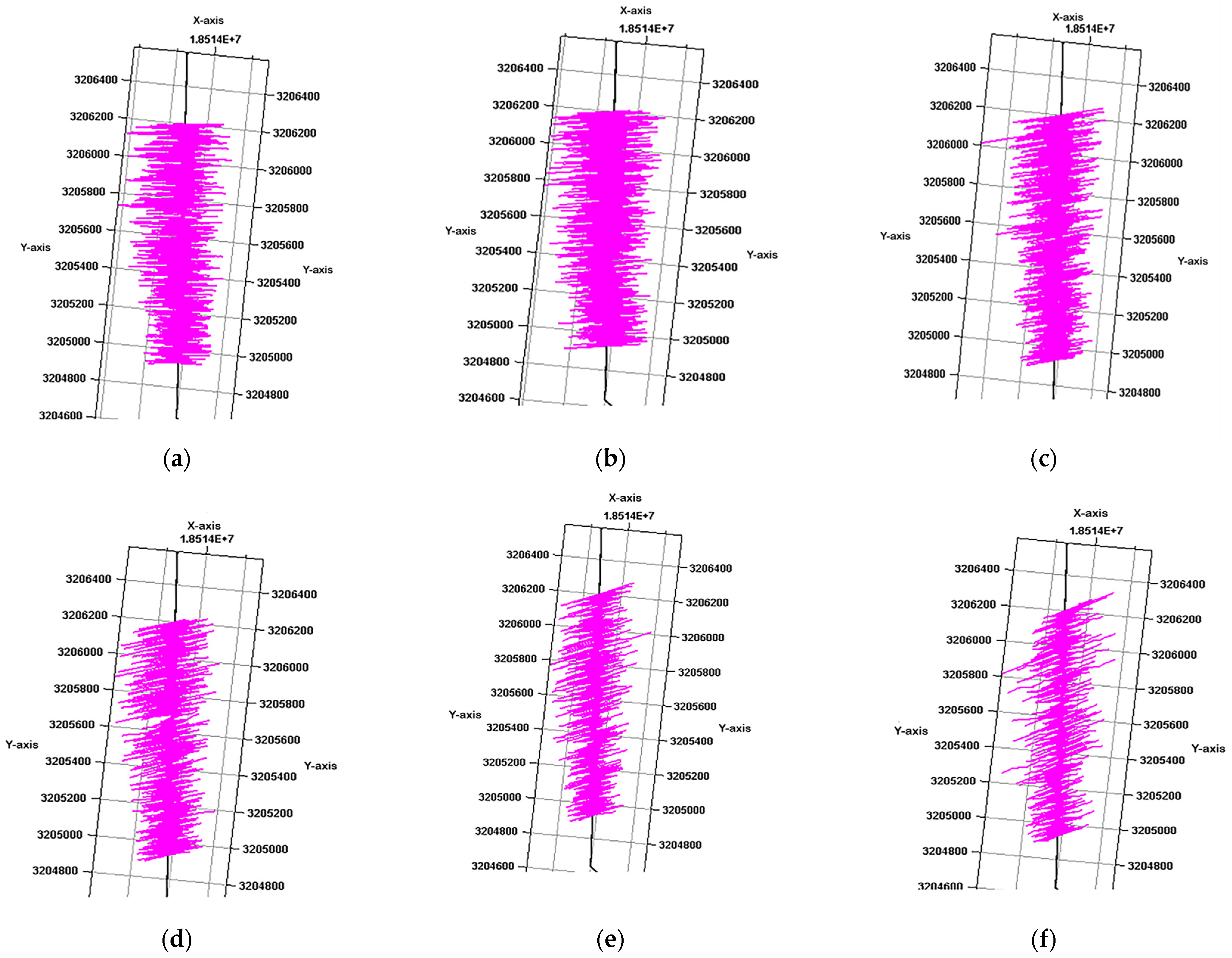
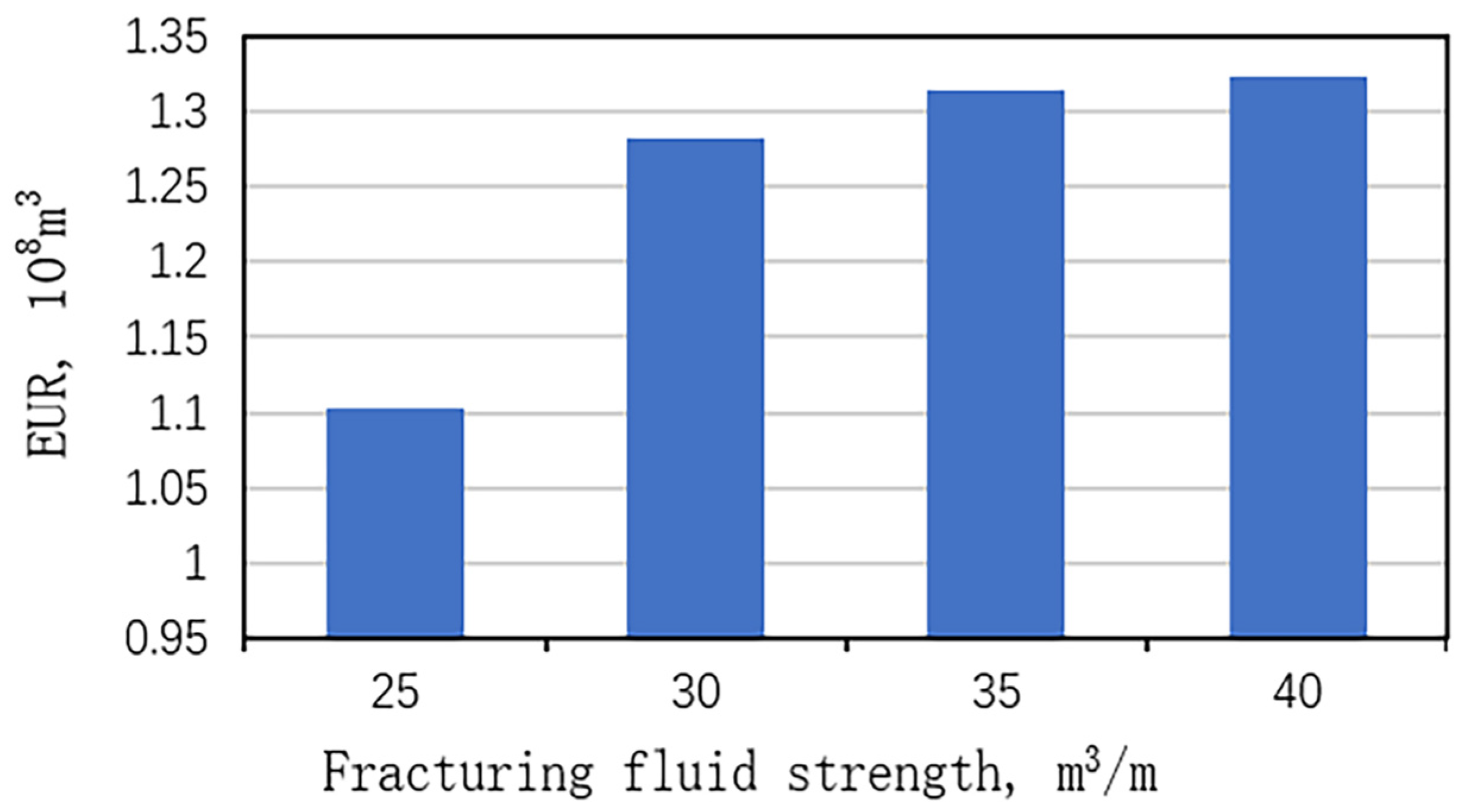
3.3. Optimization of Fracturing Fluid Strength

Figure 12 shows the fracture morphology under different fracturing fluid strengths. From the perspective of the fracture half-length, using a fluid strength of 25–40 m³/m can meet the requirements of a well spacing of 350–400 m and achieve control of inter-well resources. However, the increase in fluid strength slowed down the increase in EUR (Figure 13). The optimization range of fluid strength was determined to be 25–40 m³/m.

3.4. Optimization of Sand Addition Strength

As shown in Figure 14, with the increase of sand addition strength, the daily production of a single well significantly improved. However, when the sand addition strength reached 4 t/m and 5 t/m, the daily yield increment decreased significantly. Therefore, under the current technological and economic conditions, there may be a turning point in the influence of sand addition strength. The production after fracturing and EUR of a single well did not increase monotonically with the increase of sand addition strength.

Given the above situation, we simulated the fracture propagation and bottom-hole pressure under different sanding intensities, as shown in Figure 15 and Figure 16. At a sand addition strength of 2 t/m, which was significantly lower than the current stage, the bottom-hole pressure was about 98 MPa. When the sand strength gradually increased to 3 t/m, the increase in construction pressure was about 1–2 MPa. But when the sand addition strength increased to 4 t/m, the bottom-hole pressure continued to increase by about 3–5 MPa, and it reached the construction limit pressure. As the sanding strength continued to increase to 5 t/m, there was a significant increase in bottom hole construction pressure, which may exceed the working capacity of the equipment. Therefore, the sand addition strength in the neighboring area should be set between 3 t/m and 5 t/m.

3.5. Optimization of Construction Displacement

As shown in Figure 17, the construction displacement of segmented cluster fracturing in shale gas horizontal wells was a process parameter that did not have a significant turning point. At higher construction displacement, shale does not experience the problem of uncontrolled fracture height similar to conventional reservoirs. The sand-carrying capacity of the fracturing fluid gradually increases as the displacement increases. However, the displacement is also controlled by the equipment’s capabilities. Based on the previous development understanding, the displacement should be at least 14 m³/min to ensure smooth sand addition and a certain scale of the fracture network. At the same time, combining the equipment limit of on-site construction and the friction calculation of casing fracturing construction, it was concluded that the construction displacement limit of segmented and clustered fracturing construction in shale gas horizontal wells was around 20 m³/min. Therefore, the recommended construction displacement setting range was 14–20 m³/min.

3.6. Orthogonal Analysis Experiment

In the previous explanation, the fracturing construction parameters of adjacent wells were determined within an appropriate range. What we need to do next is to screen out the parameter levels that can maximize EUR for the Class II reservoir with the widest distribution in the neighboring area.

The classification criteria for different types of reservoirs are shown in

Table 2. Classification criteria for advantageous areas.

Favorable Area	Reservoir Thickness	Porosity	Gas Saturation	Adsorption Gas Content	Rock Density
	m	%	%	m3/t	g/cm3
I	17.4	5.6	66	2.2	2.5
II	12.7	3.7	49	2.4	2.6
Favorable Area	Area	Adsorbed Gas Storage Capacity	Free Gas Reserves	Geological Reserves	Reserve Abundance
	km2	108 m3	108 m3	108 m3	108 m3/km2
I	780	729.8	1902.6	2632.4	3.4
II	216	167.8	191.8	359.5	1.8

. The Class II reservoirs from typical cases were extracted as alternative research objects for neighboring areas. The orthogonal experimental method was used to evaluate and optimize multiple fracturing construction parameters, and the results are shown in

Table 3. Orthogonal experimental simulation results.

Number	Displacement, m3/min	Fracturing Fluid Strength, m3/m	SandAddition, t/m	Segment Length, m	Cluster Spacing, m
1	14	25	3	40	6
2	14	30	3.4	60	7
3	14	35	3.8	80	8
4	14	40	4.2	100	9
5	16	25	3.4	80	9
6	16	30	3	100	8
7	16	35	4.2	40	7
8	16	40	3.8	60	6
9	18	25	3.8	100	7
10	18	30	4.2	80	6
11	18	35	3	60	9
12	18	40	3.4	40	8
13	20	25	4.2	60	8
14	20	30	3.8	40	9
15	20	35	3.4	100	6
16	20	40	3	80	7

. The range analysis method was used to calculate and determine the results of orthogonal experiments. The calculation formulas are shown in Equations (1) and (2):

$${\overline{K}}_{jm}={\displaystyle \frac{K_{jm}}{m}}={\displaystyle \frac{V_{j1}+V_{j2}+\cdots V_{jm}}{m}}$$

(1)

where $V_{jm}$ is the experimental indicator value corresponding to the level m of the jth influencing factor. $K_{\mathit{jm}}$ is the sum of the experimental indicators corresponding to the level m of the jth influencing factor. ${\overline{K}}_{\mathit{jm}}$ is the average of $K_{\mathit{jm}}$.

$$R_j={\displaystyle \frac{\max ({\overline{K}}_{j1},{\overline{K}}_{j2},\cdots {\overline{K}}_{jm})-\min ({\overline{K}}_{j1},{\overline{K}}_{j2},\cdots {\overline{K}}_{jm})}{{\Delta }_j}}$$

(2)

where R_j is the range of the jth influencing factor that eliminates the numerical influence. ${\Delta }_j$ is the difference between the different levels of the jth influencing factor.

The level values of various factors and final range calculation results are shown in

Table 4. Range analysis table.

Level	Displacement	Fracturing Fluid Strength	Sand Addition	Segment Length	Cluster Spacing
K1(×108)	2.18	2.11	2.14	1.41	1.63
K2(×108)	2.06	2.34	2.52	2.36	2.31
K3(×108)	2.36	2.31	2.19	2.44	2.55
K4(×108)	1.99	1.83	1.74	2.38	2.1
$\overline{K}$1(×108)	0.55	0.53	0.54	0.35	0.41
$\overline{K}$2(×108)	0.52	0.59	0.63	0.59	0.58
$\overline{K}$3(×108)	0.59	0.58	0.55	0.61	0.64
$\overline{K}$4(×108)	0.50	0.46	0.44	0.60	0.53
Optimum Level	18 m3/min	30 m3/m	3.4 t/m	80 m	8 m
Rj(×108)	0.05	0.03	0.49	0.01	0.12
Primary and Secondary Sequences	Sand Addition > Cluster Spacing > Displacement > Fracturing Fluid Strength > Segment Length

, Figure 18 and Figure 19.

According to the range analysis results, the impact intensity of fracturing construction parameters was determined as follows: (1) sand addition strength, (2) cluster spacing, (3) displacement, (4) fluid strength, and (5) horizontal segment length. Based on the analysis of the optimal level, the optimal combination of fracturing parameters for Class II favorable reservoirs was sand strength of 3.4 t/m, cluster spacing of 8 m, displacement of 18 m³/min, fluid strength of 30 m³/m, and horizontal segment length of 80 m. Therefore, the construction strength plan for Class II reservoirs is shown in

Table 5. Summary of construction intensity plan.

Construction Parameters	Normal Intensity	Casing Damage Situation
Horizontal Segment Length	80 m	80~100 m
Cluster Spacing	8 m	≥10 m
Fluid Strength	30 m3/m	20~25 m3/m
Sand Addition Strength	3.4 t/m	2.5~3 t/m
Construction Displacement	18 m3/min	14~16 m3/min

. The lower reformation strength was adopted to target casing vulnerable segments.

3.7. Instance Application

In order to verify the accuracy of the optimal fracturing construction parameters for Class II reservoir simulation, a neighboring well was selected as an example for comparison, as shown in Figure 20. It can be seen that the daily gas production obtained from the integrated simulation fitted well with the initial production of the example. This showed that the geological engineering integration simulation work carried out in this paper was reliable.

4. Conclusions

This article proposes a geological engineering integrated simulation method that considers pre-fracturing parameters, which is very effective in optimizing the EUR of shale gas reservoirs. The relationship between fracturing engineering and well production capacity has been studied in detail, and the following conclusions have been obtained:

• By using the integrated geological-engineering simulation method, accurate fitting of the production history of existing wells can be achieved.
• Based on the geological model of a typical well, the reasonable range of fracturing construction parameters in the adjacent area has been determined. The specific details are as follows: horizontal well length of 40~100 m, cluster spacing of 5–10 m, fracturing fluid strength of 25–40 m³/m, construction displacement of 14 m³/min–20 m³/min, and sand addition of 3 t/m–5 t/m.
• The optimal fracturing construction parameters for Class II reservoirs have been determined by using the orthogonal experimental method. The primary and secondary relations of the parameters are sorted, that is: (1) sand addition strength, (2) cluster spacing, (3) construction displacement, (4) fracture fluid strength, and (5) horizontal segment length.
• The screened fracturing construction parameters are used for integrated simulation. The comparison between simulation results and the actual well data verifies the correctness of the selected construction parameters.

References

1. Hu, H.Y.; He, Z.D.; Chen, B.C. Accumulated Conditions of Shale Gas in the Middle-Low Palaeozoic, Yangtze Platform, China. Adv. Mater. Res. 2012, 524–527, 122–125. [Google Scholar]
2. Huang, J.; Zou, C.; Li, J.; Dong, D.; Wang, S.; Wang, S.; Cheng, K. Shale gas generation and potential of the Lower Cambrian Qiongzhusi Formation in the Southern Sichuan Basin, China. Pet. Explor. Dev. 2012, 39, 75–81. [Google Scholar] [CrossRef]
3. Tang, H.-M.; Wang, J.-J.; Zhang, L.-H.; Guo, J.-J.; Chen, H.-X.; Liu, J.; Pang, M.; Feng, Y.-T. Testing method and controlling factors of specific surface area of shales. J. Pet. Sci. Eng. 2016, 143, 1–7. [Google Scholar] [CrossRef]
4. Liu, Y.; Jin, J.; Pan, R.; Li, X.; Zhu, Z.; Xu, L. Normal Pressure Shale Gas Preservation Conditions in the Transition Zone of the Southeast Basin Margin of Sichuan Basin. Water 2022, 14, 1562. [Google Scholar] [CrossRef]
5. Wan, C.; Song, Y.; Li, Z.; Jiang, Z.; Zhou, C.; Chen, Z.; Chang, J.; Hong, L. Variation in the brittle-ductile transition of Longmaxi shale in the Sichuan Basin, China: The significance for shale gas exploration. J. Pet. Sci. Eng. 2022, 209, 109858. [Google Scholar] [CrossRef]
6. Yang, P.; Yu, Q.; Mou, C.; Wang, Z.; Liu, W.; Zhao, Z.; Liu, J.; Xiong, G.; Deng, Q. Shale gas enrichment model and exploration implications in the mountainous complex structural area along the southwestern margin of the Sichuan Basin: A new shale gas area. Nat. Gas Ind. B 2021, 8, 431–442. [Google Scholar] [CrossRef]
7. He, X.; Chen, G.; Wu, J.; Liu, Y.; Wu, S.; Zhang, J.; Zhang, X. Deep shale gas exploration and development in the southern Sichuan Basin: New progress and challenges. Nat. Gas Ind. B 2023, 10, 32–43. [Google Scholar] [CrossRef]
8. Dong, D.; Liang, F.; Guan, Q.; Jiang, Y.; Zhou, S.; Yu, R.; Zhang, S.; Qi, L.; Liu, Y. Development model and identification of evaluation technology for Wufeng Formation–Longmaxi Formation quality shale gas reservoirs in the Sichuan Basin. Nat. Gas Ind. B 2023, 10, 165–182. [Google Scholar] [CrossRef]
9. Yuan, J.L.; Deng, J.G.; Tan, Q.; Hu, L.B. A New Calculation Method for Micro-Hole Collapse Pressure of Shale Gas Reservoirs in Thrust Fault. Appl. Mech. Mater. 2013, 318, 410–413. [Google Scholar]
10. He, L.; Chen, Y.; Zhao, H.; Tian, P.; Xue, Y.; Chen, L. Game-based analysis of energy-water nexus for identifying environmental impacts during Shale gas operations under stochastic input. Sci. Total Environ. 2018, 627, 1585–1601. [Google Scholar] [CrossRef]
11. She, H.; Hu, Z.; Qu, Z.; Zhang, Y.; Guo, H. Determination of the Hydration Damage Instability Period in a Shale Borehole Wall and Its Application to a Fuling Shale Gas Reservoir in China. Geofluids 2019, 2019, 3016563. [Google Scholar] [CrossRef]
12. Zhao, J.; Peng, Y.; Li, Y.; Xiao, W. Analytical model for simulating and analyzing the influence of interfacial slip on fracture height propagation in shale gas layers. Environ. Earth Sci. 2015, 73, 5867–5875. [Google Scholar] [CrossRef]
13. Peng, Y.; Zhao, J.; Sepehrnoori, K.; Li, Z. Fractional model for simulating the viscoelastic behavior of artificial fracture in shale gas. Eng. Fract. Mech. 2020, 228, 106892. [Google Scholar] [CrossRef]
14. Li, Z.; Duan, Y.; Peng, Y.; Wei, M.; Wang, R. A laboratory study of microcracks variations in shale induced by temperature change. Fuel 2020, 280, 118636. [Google Scholar] [CrossRef]
15. Peng, Y.; Luo, A.; Li, Y.; Wu, Y.; Xu, W.; Sepehrnoori, K. Fractional model for simulating Long-Term fracture conductivity decay of shale gas and its influences on the well production. Fuel 2023, 351, 129052. [Google Scholar] [CrossRef]
16. Yong, R.; Chen, G.; Yang, X.; Huang, S.; Li, B.; Zheng, M.; Liu, W.; He, Y. Profitable development technology of the Changning-Weiyuan National Shale Gas Demonstration Area in the Sichuan Basin and its enlightenment. Nat. Gas Ind. B 2023, 10, 73–85. [Google Scholar] [CrossRef]
17. Hu, P.; Geng, S.; Liu, X.; Li, C.; Zhu, R.; He, X. A three-dimensional numerical pressure transient analysis model for fractured horizontal wells in shale gas reservoirs. J. Hydrol. 2023, 620, 129545. [Google Scholar] [CrossRef]
18. Ning, Y.; Zhang, K.; He, S.; Chen, T.; Wang, H.; Qin, G. Numerical modeling of gas transport in shales to estimate rock and fluid properties based on multiscale digital rocks. Energy Procedia 2019, 158, 6093–6098. [Google Scholar] [CrossRef]
19. Rao, X.; Zhan, W.T.; Zhao, H.; Xu, Y.F.; Liu, D.; Dai, W.X.; Gong, R.; Wang, F. Application of the least-square meshless method to gas-water flow simulation of complex-shape shale gas reservoirs. Eng. Anal. Bound. Elem. 2021, 129, 39–54. [Google Scholar] [CrossRef]
20. Shin, H.; Nguyen-Le, V.; Kim, M.; Shin, H.; Little, E. Development of Production-Forecasting Model Based on the Characteristics of Production Decline Analysis Using the Reservoir and Hydraulic Fracture Parameters in Montney Shale Gas Reservoir, Canada. Geofluids 2021, 2021, 6613410. [Google Scholar] [CrossRef]
21. Sun, H.; Yao, J.; Gao, S.H.; Fan, D.Y.; Wang, C.C.; Sun, Z.X. Numerical study of CO2 enhanced natural gas recovery and sequestration in shale gas reservoirs. Int. J. Greenh. Gas Control 2013, 19, 406–419. [Google Scholar] [CrossRef]
22. Du, X.; Li, Q.; Xian, Y.; Lu, D. Fully implicit and fully coupled numerical scheme for discrete fracture modeling of shale gas flow in deformable rock. J. Pet. Sci. Eng. 2021, 205, 108848. [Google Scholar] [CrossRef]
23. Ibrahim, A.F. Integrated workflow to investigate the fracture interference effect on shale well performance. J. Pet. Explor. Prod. Technol. 2022, 12, 3201–3211. [Google Scholar] [CrossRef]
24. Al Shehhi, H.A.A.; Bernadi, B.; Belal Al Shamsi, A.B.Z.; Al Hammadi, S.J.; Alawadhi, F.O.; Mohamed, I.N.; Al Bairaq, A.M.; Al Hosani, M.A.; Abdullayev, A.; Roopal, A. Advanced Well Completion Strategies to Improve Gas Production Deliverability in Marginal Tight Gas Reservoirs from an Onshore Abu Dhabi Gas Field. In Proceedings of the Abu Dhabi International Petroleum Exhibition Conference, Abu Dhabi, United Arab Emirates, 15–18 November 2021. [Google Scholar]
25. Yong, R.; Wu, J.; Shi, X.; Zhuang, X.; Wen, H.; Luo, Y. Development Strategy Optimization of Ning201 Block Longmaxi Shale Gas. In Proceedings of the SPE International Hydraulic Fracturing Technology Conference and Exhibition, Muscat, Oman, 16–18 October 2018. [Google Scholar]
26. Belhaj, H.; Dhabi, A.; Mnejja, M. Hydraulic Fracture Simulation of Two-Phase Flow: Discrete Fracture Modelling/Mixed Finite Element Approach. In Proceedings of the SPE Reservoir Characterisation and Simulation Conference and Exhibition, Abu Dhabi, United Arab Emirates, 9–11 October 2011. [Google Scholar]
27. Shang, X.F.; Zhao, H.W.; Long, S.X.; Duan, T.Z. A Workflow for Integrated Geological Modeling for Shale Gas Reservoirs: A Case Study of the Fuling Shale Gas Reservoir in the Sichuan Basin, China. Geofluids 2021, 2021, 6504831. [Google Scholar] [CrossRef]
28. Fan, D.; Ettehadtavakkol, A. Semi-analytical modeling of shale gas flow through fractal induced fracture networks with microseismic data. Fuel 2017, 193, 444–459. [Google Scholar] [CrossRef]
29. Deng, H.C.; Zhou, W.; Zhou, Q.M.; Chen, W.L.; Zhang, H.T. Quantification characterization of the valid natural fractures in the 2nd Xu Member, Xinchang gas field. Acta Petrol. Sin. 2013, 29, 1087–1097. [Google Scholar]
30. Jiang, T.T.; Zhang, J.H.; Wu, H. Impact analysis of multiple parameters on fracture formation during volume fracturing in coalbed methane reservoirs. Curr. Sci. 2017, 112, 332–347. [Google Scholar] [CrossRef]
31. Song, H.; Hu, Y.; Luo, E.; He, C.; Zeng, X.; Zhang, S. Analysis and Application of Fractured Carbonate Dual-Media Composite Reservoir Model. Geofluids 2022, 2022, 6785373. [Google Scholar] [CrossRef]
32. Mahmoud, M.; Aleid, A.; Ali, A.; Kamal, M.S. An integrated workflow to perform reservoir and completion parametric study on a shale gas reservoir. J. Pet. Explor. Prod. Technol. 2020, 10, 1497–1510. [Google Scholar] [CrossRef]
33. Will, J.; Eckardt, S. Optimization of Hydrocarbon Production from Unconventional Shale Reservoirs using Numerical Modelling. Int. J. Pet. Technol. 2017, 4, 14–23. [Google Scholar] [CrossRef]
34. Xu, W.; Yu, H.; Micheal, M.; Huang, H.; Liu, H.; Wu, H. An integrated model for fracture propagation and production performance of thermal enhanced shale gas recovery. Energy 2023, 263, 125682. [Google Scholar] [CrossRef]
35. Zeng, B.; Liu, J.; Song, Y.; Zhou, X.; Guo, X.; Zhao, Z.; Li, M.; Zhou, F. Optimization of Fracturing Parameters in Changning Shale Based on a New Comprehensive Multi-Factor Analysis Method. In Proceedings of the ASME 2021 40th International Conference on Ocean, Offshore and Arctic Engineering, Virtual, 21–30 June 2021. [Google Scholar]
36. Abrams, A. Mud Design To Minimize Rock Impairment Due To Particle Invasion. J. Pet. Technol. 1977, 29, 586–592. [Google Scholar] [CrossRef]
Figure 1. Distribution of geological attribute models: (a) Porosity; (b) Permeability; (c) Water saturation; (d) Poisson ratio; (e) Young’s modulus; (f) Maximum horizontal principal stress.
Energies 17 03644 g001aEnergies 17 03644 g001b
Figure 2. Simulation results of N03 well fracture propagation.
Energies 17 03644 g002
Figure 3. The historical fitting curve of N03 well.
Energies 17 03644 g003
Figure 4. Predicting final pressure distribution under different well spacing conditions: (a) 250 m; (b) 350 m; (c) 450 m; (d) 550 m.
Energies 17 03644 g004
Figure 5. The variation law of EUR under different well spacing conditions.
Energies 17 03644 g005
Figure 6. Natural fractures and maximum horizontal principal stress.
Energies 17 03644 g006
Figure 7. Fracture distribution under different angles between the well and the maximum horizontal principal stress: (a) Included angle 90°; (b) Included angle 85°; (c) Included angle 80°; (d) Included angle 75°; (e) Included angle 70°; (f) Included angle 65°.
Energies 17 03644 g007
Figure 8. Distribution of formation pressure at the end of production under different angles between the well and the maximum horizontal principal stress: (a) Included angle 90°; (b) Included angle 85°; (c) Included angle 80°; (d) Included angle 75°; (e) Included angle 70°; (f) Included angle 65°.
Energies 17 03644 g008aEnergies 17 03644 g008b
Figure 9. The relationship between EUR and well trajectory direction.
Energies 17 03644 g009
Figure 10. Statistics of average fracture half-length under different segment length and cluster spacing conditions.
Energies 17 03644 g010
Figure 11. Changes in fracture width under different cluster spacing conditions: (a) Cluster spacing is 5 m; (b) Cluster spacing is 6 m; (c) Cluster spacing is 7 m; (d) Cluster spacing is 8 m.
Energies 17 03644 g011
Figure 12. Fracture half-lengths formed by different fluid strengths under current process parameter conditions: (a) Cluster spacing is 5 m; (b) Cluster spacing is 6 m; (c) Cluster spacing is 7 m; (d) Cluster spacing is 8 m.
Energies 17 03644 g012
Figure 13. Changes in single well EUR under different fracturing fluid strengths.
Energies 17 03644 g013
Figure 14. Comparison of single well production decline curves under different sand additions.
Energies 17 03644 g014
Figure 15. Fracture propagation under different sand addition strengths: (a) 2 t/m; (b) 3 t/m; (c) 4 t/m; (d) 5 t/m.
Energies 17 03644 g015
Figure 16. Bottom hole pressure of fracturing construction under different sand addition strengths.
Energies 17 03644 g016
Figure 17. Simulation of fracture propagation under different construction displacements: (a) 14 m3/min; (b) 16 m3/min; (c) 18 m3/min; (d) 20 m3/min.
Energies 17 03644 g017aEnergies 17 03644 g017b
Figure 18. The K ¯ of various factors: (a) Construction displacement; (b) Fluid strength; (c) Cluster spacing; (d) Segment length; and (e) Sand addition.
Energies 17 03644 g018
Figure 19. Range analysis of various factors.
Energies 17 03644 g019
Figure 20. Comparison of integrated simulation results and example.
Energies 17 03644 g020